

1. INTRODUCTION
Glaciers on and around the Tibetan Plateau (TP) are crucial sources of water for Asia's glacier-fed catchments (Immerzeel and others, Reference Immerzeel, van Beek and Bierkens2010; Kaser and others, Reference Kaser, Großhauser and Marzeion2010), but are retreating and losing mass (Yao and others, Reference Yao2012; Gardner and others, Reference Gardner2013). Lack of information about changes in the mass of TP glaciers is one of the main causes of uncertainty regarding the contributions made by glaciers to current and future rises in sea level (Sugiyama and others, Reference Sugiyama, Fukui, Fujita, Tone and Yamaguchi2013). Glacier mass balance can be determined using various methods, including glaciological, geodetic and hydrological–meteorological methods. Glaciological and geodetic measurements provide two of the most commonly used methods (Hoinkes, Reference Hoinkes1970; Wang and others, Reference Wang, Li, Li, Wang and Yao2014). Surface mass-balance measurements can be reliably performed in the field using the glaciological method (Østrem and Brugman, Reference Østrem and Brugman1991; Cogley and others, Reference Cogley2011). In situ field data are important because of the uniqueness and diversity of each locality's distinct geographical conditions (Yao and others, Reference Yao2012). Nevertheless, field observations of the TP glaciers are sparse both in space and time, due to the inaccessibility and high cost of high-elevation mass-balance measurements (Ye and others, Reference Ye2015).
Fortunately, remote sensing provides the opportunity to detect glacier mass changes over time through multitemporal surface digital terrain difference analysis (‘the geodetic method’), even in remote mountainous or unreachable terrains (Paul and Haeberli, Reference Paul and Haeberli2008). However, these studies have yielded significantly different estimates with varying uncertainties (Gardner and others, Reference Gardner2013). In order to reduce the impact of such methodological uncertainties, it is recommended that the mass-balance values obtained using the glaciological method should be compared to, and calibrated using, the geodetic change in ice volumes (Zemp and others, Reference Zemp, Hoelzle and Haeberli2009; Paul and others, Reference Paul2013; Zemp and others, Reference Zemp2013).
Many current assessments of glacier change and field observations have focused on the southern and inner TP (Yao and others, Reference Yao2012; Sugiyama and others, Reference Sugiyama, Fukui, Fujita, Tone and Yamaguchi2013; Tian and others, Reference Tian2014b), with very few studies conducted in the Plateau's northern sector. Satellite remote sensing of changes in glacier coverage in the Qilian Mountains – located on the northern TP – has indicated glacier retreat over the past 50 years (Ding and others, Reference Ding, Liu, Li and Shangguan2006; Tian and others, Reference Tian, Yang and Liu2014a). Detailed analysis of any glacier retreat is difficult because essential glaciological information (e.g. ice velocity, ice thickness and mass balance) is usually unavailable.
The Ningchan No.1 Glacier (NC01), located on the northern slopes of the eastern Qilian Mountains, presents a good site for repeat field observations and an accumulation of reliable documentation for this region. The aim of this paper is to present a 5-year dataset of the mass balance, annual surface velocity and glacier thickness of NC01. We use stereo imagery 2014 from Ziyuan No.3 satellite (ZY-3), which was launched in 2012 carrying three stereo-pair image cameras (Forward, Backward, Nadir) with a resolution of 3.5/2.1 m, 1972 topographical maps and ground-penetrating radar (GPR) measurements to assess historical changes in ice volume. Measurements presented in this study will allow a better assessment and understanding of glacier mass balance in this part of the Qilian Mountains.
2. STUDY SITE
NC01 is located on the northern slope of the Lenglongling range, eastern Qilian Mountains (Fig. 1). It is a mountain glacier, and covered an area of 0.77 km2 in 1972 (Wang and others, Reference Wang1981). Its altitudinal range is 4260–4640 m a.s.l. NC01 is mainly influenced by the combined effects of the East Asian Monsoon and the Westerlies (Chen and others, Reference Chen2008). The automatic weather station established in 2010 on NC01's lateral moraine (4450 m a.s.l.) recorded a mean annual air temperature of ~−6.0°C and a mean annual precipitation (MAP) of >800 mm. According to the Chinese Glacier Inventory (Wang and others, Reference Wang1981), NC01 can be classified as a subcontinental and summer-accumulation-type mountain glacier. Over the past several decades, NC01 has experienced rapid and accelerating shrinkage (Pan and others, Reference Pan2012; Cao and others, Reference Cao2014).

Fig. 1. (a–c) Location of Ningchan No.1 Glacier on maps of (a) the Tibetan Plateau, (b) the Qilian Mountains (Mt. Qilian) and (c) the Lenglongling Mountains (Mt. LLL); (d) an overview of Ningchan No.1 Glacier as shown on satellite imagery in 2014, with the stake network. A 50 m contour interval shows the glacier surface altitude. NC01 is almost free of debris (e, f); (g) the glacier surface altitude, mass balance and surface velocity measurements made using dGPS; and (h) measurement of snow density.
3. DATA SOURCES AND METHODS
3.1. Mass balance from 2010 to 2015
3.1.1. Glaciological method
The glaciological method is used to measure mass balance based on in situ estimation of accumulation and ablation for the mass-balance year (Hoinkes, Reference Hoinkes1970; Braithwaite, Reference Braithwaite2002). The glacier mass balance for NC01 was measured following the glaciological methodology described by Østrem and Brugman (Reference Østrem and Brugman1991) using a network of stakes.
The number of ablation stakes has progressively increased on NC01, from 14 August 2010 to 22 September 2011. All stakes are located between 4250 and 4480 m a.s.l., and repositioned so as to represent nearly the entire glacier surface. They are as evenly distributed as is practicably possible at different altitudes in an attempt to accurately reflect the glacier's mass balance (Fig. 1). Annual mass balance is usually measured at the end of an ablation season (i.e. 1 September to the following 31 August), with extra stake readings taken every 1–2 months during the ablation period. Ice density in our study was assumed to be 850 ± 60 kg m−3; and the density of snow was measured in the field. Measured snow densities were neither spatially nor temporally variable, with mean values of 390 kg m−3 (with a SD of ~40 kg m−3) between 4370 and 4430 m a.s.l.
Several methods can be used to calculate the specific mass balance (b n ) of a glacier. One commonly used method is to interpolate results manually from the measured data by drawing contours of equal mass balance (Østrem and Brugman, Reference Østrem and Brugman1991; Cuffey and Paterson, Reference Cuffey and Paterson2010). In our study, areas between adjacent contours were integrated using a planimeter, and each area was assigned a constant balance value, thus:
 $$b_n = \displaystyle{1 \over S}\sum s_{i} b_{i}, \quad ( {\hbox{in m w. e}.})$$
where s i and b i represent the area between the two contours and the corresponding mass balance, respectively, and S is the total area of NC01. The hypsography of NC01 was extracted from the Digital Elevation Model (DEM) values derived from ZY-3 stereo imagery (see Section 3.3.2).
Mass balance measured using the glaciological method contains various sources of uncertainty, including the areal distribution of the stakes (Cogley, Reference Cogley1999; Fountain and Vecchia, Reference Fountain and Vecchia1999) and the accuracy of stake readings or density (Østrem and Brugman, Reference Østrem and Brugman1991; Jansson, Reference Jansson1999; Wagnon and others, Reference Wagnon2013). Additional sources of potential errors include the method of interpolation (Hock and Jensen, Reference Hock and Jensen1999) and the extrapolation method applied to unsurveyed areas. These methods are known to have an uncertainty of ~0.1–0.6 m w.e. (Jansson, Reference Jansson1999; Zemp and others, Reference Zemp, Hoelzle and Haeberli2009). As in Thibert and others (Reference Thibert, Blanc, Vincent and Eckert2008), measurement errors and sampling errors were calculated separately. Averaged over the glacier surface and the study period, we obtained a mean uncertainty of ~0.5 m w.e. a−1 for the glacier-wide mass balance, and 1.1 m w.e. for the cumulative mass balance.
3.1.2. Geodetic method
The geodetic method is an indirect method of determining glacier volume balance. The surface elevations of a glacier at two or more different times are compared, and the differences are then used to determine mass balance over the respective time period by assuming an appropriate density. To measure changes in the elevation of the glacier surface in the field, our field team performed real-time kinematic (RTK) GPS measurements in 2010, 2013 and 2015 using a pair of 5800 RTK-type differential GPS (dGPS) units manufactured by Trimble Company (Fig. 2). We first installed a GPS receiver base station on a boulder close to the glacier (<5 km away). The position of this station was marked with red paint, in order to facilitate re-measurement. The other GPS receiver was used to measure point positions on the glacier surface. The dGPS units were connected by a radio signal, enabling the RTK survey to be carried out with mm-level accuracy.

Fig. 2. dGPS measurement tracks and validation points (red) for the years 2010, 2013 and 2015. The pink polygon is the subset area for comparing geodetic and glaciological mass balance.
The GPS data were re-projected to the Universal Transverse Mercator (UTM) coordinate system, then referenced to the World Geodetic System 1984 (WGS84) datum. Point elevation data were subsequently interpolated using the Ordinary Kriging method to produce a DEM. The relative altitudinal differences between the two DEMs were then compared. The resulting highly accurate measurement of change in altitude between the two DEMs reflected the difference over time in glacier thickness.
Two errors can occur during the execution of this approach: one error can arise from the employment of the dGPS units themselves, and the other from the measurement procedure. Since we kept the distance between the base and the roving GPS receivers <5 km, the estimated error was within ±2 cm horizontally, and ±3 cm vertically. Minor errors may be introduced in the calculation of elevation if the glacier surface is not horizontal. The degree of error depends on the gradient of the glacier surface (Tian and others, Reference Tian2014b). We therefore chose glacier points for measurement where the surface was quite flat, yielding an estimated maximum error of ±2 cm. The maximum error in measurement should therefore be <±5 cm.
However, when we use these points to create a DEM, the error will be larger, as it will be controlled by the number of points used, and whether or not their distribution is uniform. We therefore randomly chose 30 points from the NC01 Glacier to examine the DEMs. The survey points are relatively densely distributed in the study area. The mean altitudinal error was therefore small, at ~0.5 m (Cao and others, Reference Cao2014). According to the law of error propagation, the final uncertainty of the geodetic surface balance was ±0.71 m (±0.6 m w.e.).
3.2. Surface velocity
Annual surface ice velocities were measured every year in late August or early September on NC01 by determining the locations of the stakes using dGPS. The method employed was the same as the Geodetic Method outline in Section 3.1.2. The glacier velocity error was calculated to be ~5 cm a−1.
3.3 Glacier area
Pan and others (Reference Pan2012) investigated the outlines of glaciers in the region using remote-sensing imageries for the period 1972–2007. We expand this analysis to include manually digitized glacier outlines from ZY-3 imagery collected in 2014.
The accuracy of the measurement of glacier outlines can be strongly influenced by the different spatial resolutions of the satellite datasets used (Paul and others, Reference Paul2013). We estimated the uncertainty using a buffer of 10 m for topographical maps and ZY-3 imagery (cf. Bolch and others, Reference Bolch2012; Shangguan and others, Reference Shangguan2015). We assumed that any uncertainty arising from image co-registration could be captured using the buffer method.
3.4. Ice thickness
3.4.1. GPR dataset (2014) and glacier thickness
GPR has previously been used to measure glacier thickness, infer bed topography, and examine glacier internal structure and other snow and ice properties (Arcone and others, Reference Arcone, Lawson, Delaney and Delaney1995; Pälli and others, Reference Pälli2002; Prinz and others, Reference Prinz, Fischer, Nicholson and Kaser2011; Hagg and others, Reference Hagg, Mayer, Lambrecht, Kriegel and Azizov2013; Sugiyama and others, Reference Sugiyama, Fukui, Fujita, Tone and Yamaguchi2013). GPR field measurements were performed in August 2014 using a pulse EKKO PRO system (Canadian Sensors and Software, Inc., Ontario). We used 100 MHz frequency antennas, with a 4 m separation between the two antennas. The ice thickness is computed using the two-way travel time between GPR and glacier–bedrock interface by assuming a wave velocity through the glacier's ice of 0.169 m ns–1 (Wang and others, Reference Wang2015). The thickness data were interpolated by the Ordinary Kriging method to produce a raster of glacier thickness with the same projection as the DEMs.
The horizontal positions of the GPR measurement points were recorded using a handheld Trimble GeoXT 6000 with a horizontal accuracy of 0.5–2 m, sufficient for the size of the GPR footprint. The altitudes of the positions recorded were taken from the DEM created using the dGPS. In addition, any possible uncertainty in the reflection peaks in the radargram was taken to be 0.9 m from the repeated identification of the locations of these peaks. We also built in expected uncertainties due to any possible ambiguity in the wave velocity, GPS positioning errors and/or any vertical resolution limited by the adopted wavelength value. Totaling these, the maximum uncertainty in ice thickness measurement was estimated to be 2 m ± 2% of the actual ice thickness (Sugiyama and others, Reference Sugiyama, Fukui, Fujita, Tone and Yamaguchi2013).
3.4.2. Glacier surface elevation data and ice volume change
A topographical map (scale 1: 50 000) from the Chinese State Bureau of Surveying and Mapping produced using aerial photography in 1972 was used to create a DEM for comparison with the collected modern surface data. This DEM was generated from a series of altitudinal points digitized from the contours (of interval 20 m) marked on the topographical map (Pan and others, Reference Pan2012). In order to compare the results with other data, the DEM was re-projected on to the WGS84 UTM using a seven-parameter datum transformation model (Wang and others, Reference Wang, Wang and Lu2003).
We collected ZY-3 stereo-pair images (for 24 July 2014) and then generated a DEM of the study area using the ‘DEM Extraction Model’ included in the ENVI 5.0 software, using the geographical reference system WGS84 UTM, Zone 47 N. During the generation of the DEM, 20 ground control points (GCPs) were selected; the coordinates and altitudes of these GCPs were derived from Landsat 8 scenes and the DEM built in 1972.
Multitemporal DEMs require co-registration prior to differential analysis in order to remove any horizontal and/or vertical offsets (Pieczonka and others, Reference Pieczonka, Bolch, Wei and Liu2013). An analytical method proposed by Nuth and Kääb (Reference Nuth and Kääb2011) and proven as effective by (Paul and others, Reference Paul2015) was used in this study. In ice-free areas, co-registration between the 1972 DEM and the DEM constructed using ZY-3 imagery was implemented using a shifting vector (dx = 10.4 m, dy = −32.3 m); the altitudinal shift was then calculated based on the relation between this result and the altitudinal difference. After co-registration, the obtained accuracy of 1.8 m implied that post-processed DEMs can be applied to estimates of changes in glacier ice volumes.
4. RESULTS
4.1. Glacier mass balance and ELA, from 2010 to 2015
The mass-balance year starts in early autumn and ends in late summer. Figure 3 shows the mass balance recorded at stakes on NC01 from September 2010 to September 2015, as well as changes in annual and cumulative mass balances, calculated using the stake method. Annual mass balance varies between −1.48 ± 0.5 m w.e. (2012/13) and −0.15 ± 0.5 m w.e (2014/15), with a mean of −0.90 ± 0.5 m w.e. The cumulative mass balance was ~−4.50 ± 1.1 m w.e. from September 2010 to September 2015.
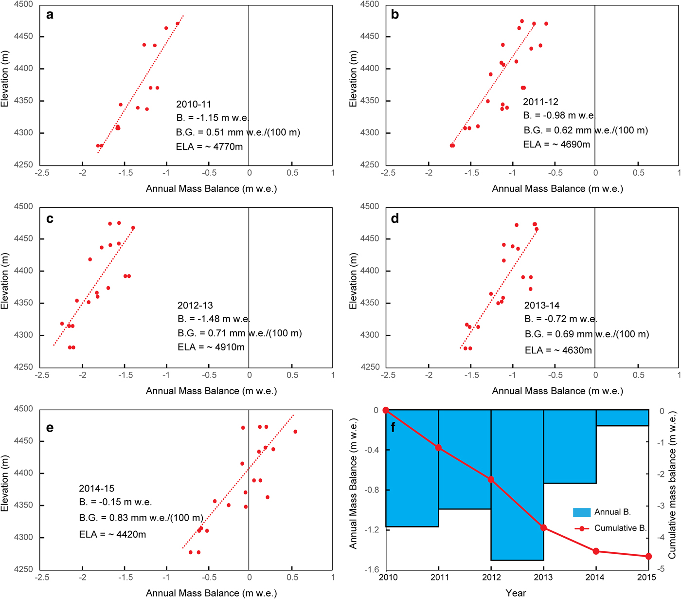
Fig. 3. (a–e) Five years’ worth of annual point mass-balance values as a function of altitude derived from the field measurements collected on NC01. Linear regression lines were used to derive the annual glacier-wide mass balance B. (f) Annual (blue histograms) and cumulative (red lines with red dots) mass balances of NC01 from 2010 to 2015.
Equilibrium line altitudes (ELAs) (the altitude where annual mass balance was zero) were determined though linear interpolation/extrapolation of the altitudinal profile of annual mass balance. In four of the five observation years, the ELA was greater than the maximum elevation of the glacier (Fig. 3). In 2014–15, the ELA was ~4420 m, and the average ELA was ~4680 m for the period 2010–15.
Harsh conditions and bad weather meant that dGPS measurements on the glacier could not be made each year. We measured the glacier surface elevation three times, in 2010, 2013 and 2015, but due to the complex terrain, were unable to measure the entire geographical range of the glacier. In order to compare the results obtained from using these two methods (glaciological and geodetic methods), the same part of the glacier was chosen (Fig. 3).
Using the geodetic method, the mean elevation change from 2010 to 2015 was ~−4.3 ± 0.6 m w.e. in the subregion, while the surface mass balance was ~−4.8 ± 0.5 m w.e. from the glaciological method. The difference between the two methods was 10% (0.5 m). However, the mean annual differences between the glaciologically and geodetically derived results were less than the overlap in the uncertainty of both datasets. Hence, no adjustment of the glaciological data series in relation to the volumetric one was required (Zemp and others, Reference Zemp2010).
4.2. Mean annual surface velocity
Over the relatively short time period of 2010–15, no velocity change was detectable. Mean glacier velocities were low at ~2.8 ± 0.05 m a−1 (Fig. 4), and varied with altitude. At the glacier terminus and near the summit of the glacier, the velocity was relatively slow at ~1–2 m a−1. In its central sector, the surface gradient is relatively steep, and there is correspondingly an increase in velocities. Observed ice velocities at 4340, 4370 and 4430 m a.s.l. were 3.3 ± 0.05, 3.6 ± 0.05 and 2.4 ± 0.05 m a−1, respectively.

Fig. 4. NC01 glacier GPR measurements. (a) Red points indicate the GPR measurement locations. (b) The glacier thickness distribution for this glacier. (c) Mean annual surface velocities measured during the period 2010–2015. All measurements have been averaged. The blue and red lines represent cross-sections (CS_4340, CS_4370 and CS_4430 at 4340, 4370 and 4430 m a.s.l., respectively). The flow direction is shown by red arrows.
4.3. Changes in glacier area from 1972 to 2014
From ZY-3 imagery, the total area of the NC01 glacier in 2014 can be calculated as being 0.39 ± 0.04 km2. This compares with an area of 0.77 ± 0.05 km2 in 1972 (Pan and others, Reference Pan2012), meaning that the glacier appears to have shrunk by 0.34 ± 0.06 km2 (1.05% a−1).
4.4. Glacier thickness and glacier bed morphology
We used 764 GPR points from the NC01 glacier (Fig. 4a) to interpolate glacier thickness over the whole glacier. The glacier thickness distribution map shows that the glacier thickness tends to be deepest in the central, and shallowest in the upper and bottom sectors of the glacier (Fig. 4b). The deepest ice is located along the central flowline, with the maximum ice thickness (65 ± 3.3 m) close to the central sector of the glacier and its main flowline. The mean ice thickness for the entire glacier is ~24 ± 2.5 m. Ice thickness distribution patterns and profiles across the glacier are shown in Figures 4b and 5.
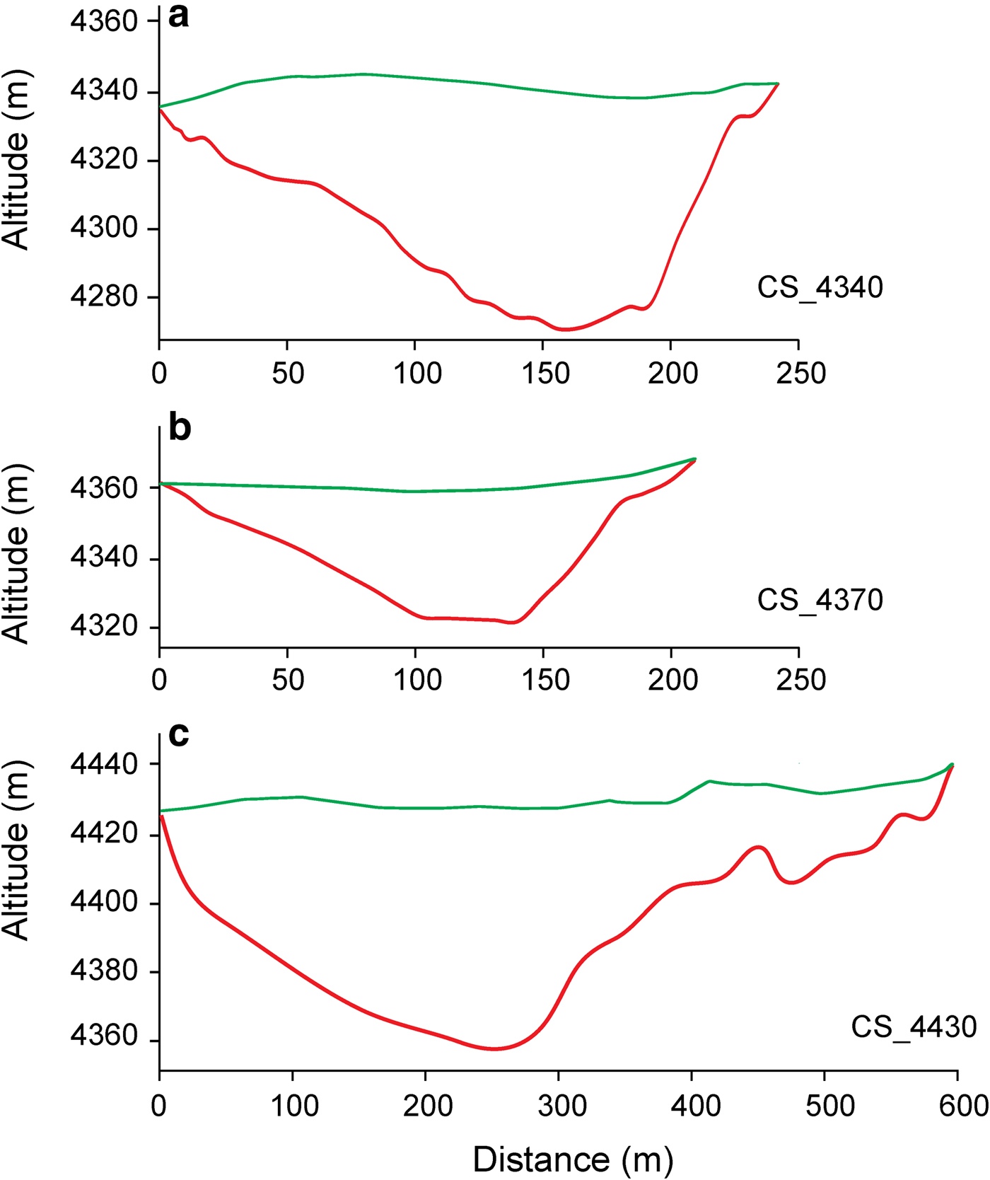
Fig. 5. Ice depths and surface topographies of the three main cross-sections CS_4340, CS_4370 and CS_4430. The graphs show the bedrock altitude a.s.l. (red line) and modern glacier surface altitude a.s.l. (green line) along the profile path. All profile locations are shown in Figure 4.
4.5. Changes in ice volume from 1972 to 2014
In 2014, the mean ice thickness was ~24 ± 2.5 m over an area of 0.39 ± 0.04 km2, corresponding to an ice volume of (9.36 ± 0.97) × 106 m3. We calculated the change in glacier thickness from the two reconstructed DEMs for the years 1972 and 2014 (Fig. 6). From 1972 to 2014, the glacier showed a significant thinning, to a maximum value of −70 ± 1.8 m. The ice volumes for glacier NC01 for 1972 were obtained by summing the estimates of 2014 ice volume and total volume change between 1972 and 2014. This gave an ice volume for 1972 of (24.32 ± 0.97) × 106 m3. From 1972 to 2014, the ice volume decreased by (14.96 ± 0.97) × 106 m3 (1.46% a−1), equivalent to a loss of mass of (12.72 ± 0.82) × 106 t w.e.

Fig. 6. The DEMs for glacier NC01 in (a) 1972, as derived from topographic maps; (b) 2014, as derived from ZY-3 images and (c) change in altitude from 1972 to 2014.
4.6. Ice fluxes
The ice flux Q (m3 of ice per year) through the cross-sections at 4340, 4370 and 4430 m a.s.l. can be inferred using two different methods. The first is the kinematic method, which involves multiplying the cross-sectional area S c (m2) with the depth-averaged horizontal ice velocity U (m a−1), thus:
 $$Q = U \; S_{\rm c}.$$
The depth-averaged horizontal ice velocity was derived from the mean surface ice velocity obtained by averaging the surface velocities available along each cross-section. Neglecting dynamic changes, the ice fluxes for each cross-section can be derived from mass-balance data (e.g. Azam and others, Reference Azam2012). In this way, we calculated ice fluxes using annual surface mass balances measured during the 2010–15 period. The ice fluxes for each cross-section as derived from mass-balance data were calculated thus:
 $$Q = \displaystyle{1 \over {0.85}}\; \; \mathop \sum \limits_z^{z_{max}} s_ib_i, $$
where Q is the ice flux (converted into m3 of ice per year using an ice density of 850 kg m−3, at a given altitude, z), and b i is the annual mass balance for the altitudinal range i shown on the map as area s i .
The ice fluxes calculated using both methods at each cross-section are given in Table 1. The ice fluxes calculated using the kinematic method are far larger than the balance fluxes calculated from the 2010–15 mean surface mass balances. Therefore, it would be safe to assume that there is likely to be further thinning and terminus retreat of glacier NC01 over the next few years (Azam and others, Reference Azam2012).
Table 1. Ice fluxes, as inferred from the kinematic method and from the mean annual surface mass-balance datasets for each cross-section
5. DISCUSSION
It is well known that climatic fluctuations are the principal cause of global glacier shrinkage (Vaughan and others, Reference Vaughan2013). Pan and others (Reference Pan2012) pointed out that the shrinkage of the NC01 glacier was also attributable to climate change. Though the period of observation is short, the observed surface mass balance from 2010 to 2015 is positively correlated with annual precipitation and negatively correlated with mean summer (JJA) air temperature observed at the Menyuan meteorological station (37°23′N, 101°37′E; 2924 m a.s.l.; ~25 km from glacier NC01; Fig. 7). A peak mean summer air temperature (13.6°C) and low MAP values (460 mm) appear to have led to a relatively highly negative surface mass balance from September 2012 to September 2013, while a lower mean summer air temperature (12.1°C) and higher MAP values (548 mm) may qualitatively explain the less negative mass-balance rate observed between September 2014 and September 2015.
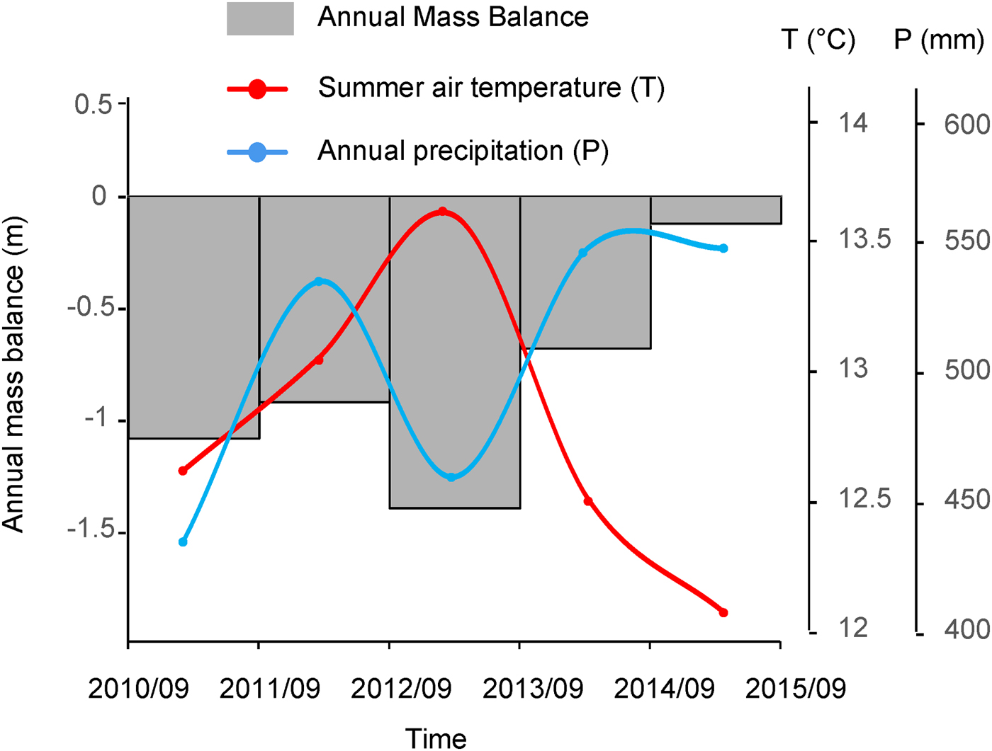
Fig. 7. Annual surface mass-balance values compared with meteorological values (summer air temperature and MAP) recorded at the Menyuan station.
We have previously thought that glacier shrinkage usually occurs principally at its terminus. However, comparing historical glacier margins shown on remote-sensing imagery with current satellite images and fieldwork shows that what was previously part of one large glacier has now become an isolated glacier (i.e. glacier NC01), with considerable shrinkage of the glacier margins near the summit. This phenomenon appears to be present in other small glaciers in this region of China (Tian and others, Reference Tian2014b; Kang and others, Reference Kang2015).
The annual surface mass balance of the NC01 glacier indicated that the glacier faces a relatively strong retreat, with a mean negative annual surface mass balance of −0.9 m w.e. from 2010 to 2015. This negative surface mass balance is greater than that for most glaciers in High Mountain Asia. According to our results, the mean glacier surface elevation lowered by 30 ± 1.8 m between 1972 and 2014. Cao and others (Reference Cao2014) used topographical maps and GPS to show that the change in altitude of NC01 was 28.8 ± 11 m from 1972 to 2010. These results are very similar.
According to the observations made at our stakes, the mean ELA for the 2010–15 period was ~4680 m a.s.l., higher than the summit of NC01. We can infer from this that glacier NC01 will completely disappear in the near future.
6. CONCLUSIONS
Based on numerous measurements, this study observed the surface mass balance of glacier NC01 from 2010 to 2015 using glaciological and geodetic methods. The two methods provided similar results: the mean annual surface mass balance from 2010 to 2015 was ~−0.90 ± 0.5 m w.e. Observed ice velocities at 4340, 4370 and 4430 m a.s.l. were 3.3 ± 0.05, 3.6 ± 0.05 and 2.4 ± 0.05 m a−1, respectively. The mean ice thickness was ~24 ± 2.5 m in 2014. From 1972 to 2014, the glacier area shrank from 0.77 ± 0.05 to 0.39 ± 0.04 km2, and the ice volume decreased by (14.96 ± 0.97) × 106 m3, equivalent to a mass loss of (12.72 ± 0.82) × 106 t w.e. over the same period. The ice fluxes calculated using the kinematic method are far larger than the balance fluxes calculated from the 2010–15 mean surface mass balances; and according to the observations, the mean ELA for the 2010–15 period was higher than the summit of NC01. We can infer that glacier NC01 will completely disappear in the near future.
ACKNOWLEDGEMENTS
This paper has benefited from valuable comments and constructive suggestions by J. Shea, M. Beedle, M.F. Azam and two referees, whose efforts are gratefully acknowledged. This study is financially supported by the National Basic Work Program of the Ministry of Science and Technology of China (grant No. 2013FY111400), the National Natural Science Foundation of China (grant No. 41701057) and Fundamental Research Funds for the Central Universities (lzujbky-2017-225).


 Open access