


1. Introduction
The existence of water beneath the Antarctic ice sheet has been known since the 1950s, when the first subglacial lakes were discovered through airborne radar sounding (Reference Robin, Swithinbank and SmithRobin and others, 1970). The most recent lakes inventory (Reference Siegert, Carter, Tabacco, Popov and BlankenshipSiegert and others, 2005) tallied 145 lakes, and many more lakes have been discovered since then (e.g. Reference Bell, Studinger, Shuman, Fahnestock and JoughinBell and others, 2007). Most of these are located near ice divides in the deep interior of the ice sheet. Reference Engelhardt, Humphrey, Kamb and FahnestockEngelhardt and others (1990) identified a subglacial water system beneath a fast-flowing ice stream, and later work investigated many of the characteristics of these systems (Reference Kamb, Alley and BindschadlerKamb, 2001), such as subglacial water pressure, character of underlying sediments, and the extent and level of hydraulic connection between two subglacial points. Basal melt rates have been estimated for some of the Antarctic ice streams (Reference Joughin, Tulaczyk and EngelhardtJoughin and others, 2003), but these calculations were made assuming the flow of subglacially generated meltwater is uniform in space and time.
There have been some key studies since the Reference Siegert, Carter, Tabacco, Popov and BlankenshipSiegert and others (2005) inventory which have demonstrated that satellite detection of surface changes can be interpreted to infer subglacial hydrologic activity (Reference Gray, Joughin, Tulaczyk, Spikes, Bindschadler and JezekGray and others, 2005; Reference Wingham, Siegert, Shepherd and MuirWingham and others, 2006; Reference Fricker, Scambos, Bindschadler and PadmanFricker and others, 2007), leading to new discoveries about the hydrologic system. These studies have revealed: (1) there can be major fluctuations in flow of subglacial water, and rapid movement of large volumes of water occurs beneath the ice sheet, via episodic ‘subglacial floods’. Movement is documented between pairs of lakes over long distances (tens of km) (Reference Gray, Joughin, Tulaczyk, Spikes, Bindschadler and JezekGray and others, 2005; Reference Wingham, Siegert, Shepherd and MuirWingham and others, 2006); (2) active lakes exist under the ice streams, therefore potentially affecting ice-flow rates and influencing ice-sheet mass balance (Reference Gray, Joughin, Tulaczyk, Spikes, Bindschadler and JezekGray and others, 2005; Reference Fricker, Scambos, Bindschadler and PadmanFricker and others, 2007); (3) subglacial systems can be widespread, with multiple reservoirs and apparent drainage systems (Reference Fricker, Scambos, Bindschadler and PadmanFricker and others, 2007); and (4) subglacial lake drainage continues to the ice grounding line, where subglacial water enters the Southern Ocean (Reference GoodwinGoodwin, 1988; Reference Fricker, Scambos, Bindschadler and PadmanFricker and others, 2007).
There is emerging evidence of a direct link between Antarctic ice-stream dynamics and subglacial lakes. Reference Bell, Studinger, Shuman, Fahnestock and JoughinBell and others (2007) showed that subglacial lakes can have a role in initiating fast ice-stream flow in the upper glacier catchments, and near the South Pole several small lakes are coincident with ice-stream onset regions (Reference Siegert and BamberSiegert and Bamber, 2000). On Byrd Glacier, Reference Stearns, Smith and HamiltonStearns and others (2008) linked a subglacial flooding event to an increase in flow speed of 10%, sustained for 14 months. The presence of water beneath an ice stream, and its action as a lubricant either between the ice and subglacial bed or between grains of a subglacial till affects ice-flow rates (Reference Kamb, Alley and BindschadlerKamb, 2001). This key process acting at the basal ice-sheet boundary is still insufficiently understood to be reliably incorporated into ice-sheet models and is therefore missing from current assessments of future ice-sheet behavior and sea-level contribution. Knowledge of subglacial water movement and flux rates is fundamental to our understanding of ice-stream dynamics, and for this reason documenting the interconnected pattern of subglacial water flow is of critical importance. Before we can incorporate processes of subglacial water flow into ice-sheet models, we require further observations, and extended observations over time. Additionally, monitoring subglacial outflows from the ice-sheet margins is important for quantifying freshwater flux to the ocean and understanding ice–ocean interactions.
Datasets for studying subglacial hydrology are limited due to the inaccessibility of the environment. Mapping active subglacial signals requires a combination of high spatial and high temporal sampling. RADARSAT interferometric synthetic aperture radar (InSAR) data were used first to identify isolated areas of elevation change due to subglacial water activity and showed displacement between two lakes on Kamb Ice Stream (Reference Gray, Joughin, Tulaczyk, Spikes, Bindschadler and JezekGray and others, 2005). This study also retrospectively interpreted some regions of large elevation change observed in upper Whillans Ice Stream, using airborne laser altimetry, (Reference Spikes, Csathó, Hamilton and WhillansSpikes and others, 2003) as resulting from subglacial lake activity. Both of these studies were limited by data availability to a single time interval. Then two breakthroughs came from satellite altimetry analysis. Using satellite radar altimetry from the European Remote-sensing Satellites (ERS-1 and -2), Reference Wingham, Siegert, Shepherd and MuirWingham and others (2006) identified a subglacial flood involving four subglacial lakes that traveled more than 290 km over a 16 month period in the Adventure Trench subglacial basin in East Antarctica. Reference Fricker, Scambos, Bindschadler and PadmanFricker and others (2007) used repeat-track analysis of Ice, Cloud and land Elevation Satellite (ICESat) laser altimetry and identified a complex, active plumbing system involving linked reservoirs under the fast-flowing portions of three large West Antarctic ice streams (Mercer, Whillans and MacAyeal Ice Streams, formerly Ice Streams A, B and E).
In this paper, we revisit the hydrologic system of lower Mercer and Whillans Ice Streams and examine its behavior since our initial study (Reference Fricker, Scambos, Bindschadler and PadmanFricker and others, 2007, based on data spanning February 2003–June 2006). Since then, four additional ICESat data acquisition periods (Table 1) and further image difference data have allowed us to extend the time series of elevation changes across each lake. With this longer record we have observed several correlated events among the larger lakes, implying a connected water system. The 4 year time series also enables us to begin to examine patterns in lake cyclicity. A new hydrostatic-potential map, based on higher-resolution surface topography from an image-enhanced digital elevation model (DEM), allows us to examine the potential pathways of water moving through the system, which we have confirmed with satellite observations (ICESat and moderate-resolution imaging spectroradiometer (MODIS) image differencing).
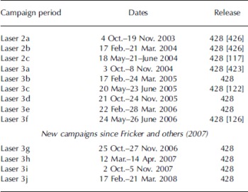
Table 1. Acquisition dates and release numbers for the thirteen 91 day ICESat campaigns acquired up to March 2008. ICESat data release numbers are of the form XYY, where X represents the quality (from 1 to 4; where 1 is initial, uncalibrated data and 4 is fully calibrated) and YY represents the data product format. Data from Laser 2a–3f campaigns were used in our earlier study (Reference Fricker, Scambos, Bindschadler and PadmanFricker and others, 2007); in some cases the data release has changed. When release numbers have changed, those used by Reference Fricker, Scambos, Bindschadler and PadmanFricker and others (2007) are given in square brackets. With the exception of Lasers 2c, 3c and 3f, the difference just reflects a change in the data product format, not in the data quality
2. Study Region
Our study region is the lower portion of Mercer and Whillans Ice Streams, West Antarctica, the same study region as Reference Fricker, Scambos, Bindschadler and PadmanFricker and others (2007) (Fig. 1). In that study, we detected several localized elevation changes using ICESat repeat-track analysis and satellite image differencing. We interpreted these elevation-change regions as surface expressions of ponded subglacial water, and the observed vertical movement to be due to water gain or loss at each lake. In that paper, we identified 14 regions of activity, and four areas large enough in area and amplitude to be called ‘subglacial lakes’. Analysis of more recent data and improvements in the algorithm we use have confirmed that the four large regions are very active and have eliminated four smaller regions that we now interpret as surface undulations advecting through the ICESat ground-track pattern with the flow of the ice. One new lake has been identified, and vertical movement at lake 10 near ice raft ‘a’, detected in the earlier study but not discussed due to uncertainty, is now included as part of the subglacial hydrologic system. Ice raft ‘a’ was first documented as an ice rise (Reference Shabtaie and BentleyShabtaie and Bentley, 1987a,Reference Shabtaie and Bentleyb), but later Reference AlleyAlley (1993) reinterpreted it as an ice raft. We have adopted informal names for the largest lakes, after the ice ridges next to which, or the ice streams under which, they are located: subglacial lakes Engelhardt (SLE), Whillans (SLW), Conway (SLC) and Mercer (SLM) (Fig. 1; Reference Fricker, Scambos, Bindschadler and PadmanFricker and others, 2007). The other five lakes in the region we refer to as Upper Subglacial Lake Conway (USLC) and lakes 7, 8, 10, and 12 (Figs 1 and 2; numbering for the lakes is from Reference Fricker, Scambos, Bindschadler and PadmanFricker and others, 2007), and we report on these in more detail in this paper.
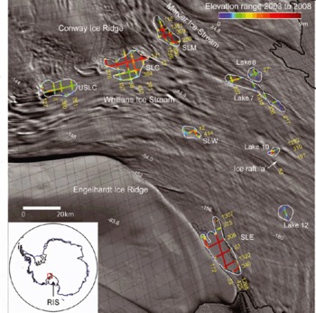
Fig. 1. Location of study region on lower Whillans and Mercer Ice Streams showing all the active regions detected through ICESat repeat-track analysis, and indicating the main lakes discussed in the text. ICESat ground tracks are shown as thin black lines, and coloured track segments represent the total range in ice surface elevation over each lake for the period 2003–08 (track segments are labelled with their track number). The major lake areas are identified by acronyms: SLM, Subglacial Lake Mercer; SLC and USLC, Subglacial Lakes Conway and upper Conway; SLW, Subglacial Lake Whillans; SLE, Subglacial Lake Engelhardt. Smaller lakes are identified by a number (e.g. lake 10, where the numbering comes from Reference Fricker, Scambos, Bindschadler and PadmanFricker and others (2007)); there are fewer active regions than shown in their figure 1, for reasons discussed in the text. Background image is MODIS Mosaic of Antarctica (MOA; Reference Scambos, Haran, Fahnestock, Painter and BohlanderScambos and others 2007), and thick black curve is the grounding line from MOA. The black line over SLM is the lake boundary as defined by Reference Carter, Blankenship, Peters, Young, Holt and MorseCarter and others (2007); the dashed part of the line is the limit of their data.
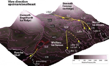
Fig. 2. Hydrostatic-potential contour map over study region derived from new DEM. Greyscale, perspective elevation, and contours indicate potential pressure in kPa, with a contour interval of 100 kPa. The outlines of the four major lakes are shown (SLE: red; SLW: blue; SLC: yellow; SLM: green); other active regions are outlined in white. White curve is break-in-slope associated with the grounding line (from MOA; Reference Scambos, Haran, Fahnestock, Painter and BohlanderScambos and others 2007). The proposed flow direction and lake linkages are indicated with yellow arrows.
Some of the lakes in the system have been previously surveyed during airborne field campaigns. SLM was identified by Reference Carter, Blankenship, Peters, Young, Holt and MorseCarter and others (2007) as a ‘definite’ lake (one exhibiting all appropriate characteristics) in an analysis of airborne radar sounding data collected in 1998/99. Their classification scheme uses radar reflection properties to characterize basal ice and bed reflections (e.g. the high dielectric contrast between liquid water and ice). In Reference Carter, Blankenship, Peters, Young, Holt and MorseCarter and others' (2007) scheme, ‘definite’ lakes have higher-amplitude returns than their surroundings by at least 2 dB and are both consistently reflective (specular) and have an absolute reflection coefficient greater than −10 dB. Our shoreline of SLM derived from satellite analysis matches the region of lake radar return from Reference Carter, Blankenship, Peters, Young, Holt and MorseCarter and others (2007) to within 2 km. SLC was also surveyed during the 1998/99 campaign, but was not classified as a lake by Reference Carter, Blankenship, Peters, Young, Holt and MorseCarter and others' (2007) scheme. This is because there was no obvious return from the ice–water interface, perhaps due to surface crevassing. Similarly, a single airborne radar profile acquired over SLE in January 1998 also showed no evidence of a lake, but did show effects of intense surface crevassing (Reference Fricker, Scambos, Bindschadler and PadmanFricker and others, 2007, supplementary online material). Intense near-surface scattering may mask the bed return by scattering the radar energy. For both of these lakes (SLC and SLE), no surface crevassing is observed in either MODIS or SAR imagery; however, both lakes are adjacent to the heavily crevassed shear margins of Whillans Ice Stream.
3. Methods
3.1. Surface elevation change from ICESat
ICESat was launched in January 2003 and carries the Geoscience Laser Altimeter System (GLAS) instrument. This is the first laser altimeter to be flown in a near-polar orbit, acquiring data over a latitude range of 86.0° S to 86.0° N. Since 4 October 2003, ICESat has operated in a 91 day exact repeat orbit with a 33 day subcycle. Flying in this orbit, ICESat has acquired data ‘campaign-style’, repeating the same 33 day section of the 91 day orbit two or three times per year (Table 1). For this study we use Release 428 data, which was the most recent release at the time of analysis.
The ICESat laser (1064 nm) fires at 40 Hz, producing a ground spot every ∼172 m along-track, with a footprint size of 50–70 m. For the Antarctic ice sheet, the elevation error for individual ICESat measurements is 15 cm (Reference ShumanShuman and others, 2006). We obtain geolocated GLAS footprint locations, ocean and load tide corrections, and energy and gain information from the GLA12 product. We apply a saturation correction to the elevations for all points where receiver gain was equal to 13 and the return energy was greater than 13.1 × 10⁻¹⁵ J (Reference Sun, Abshire and YiSun and others, 2003). This correction can be tens of centimeters (Reference Fricker, Borsa, Minster, Carabajal, Quinn and BillsFricker and others, 2005). The saturation correction is now available as a parameter in the GLA12 product.
ICESat repeat-track analysis
Following the technique used by Reference Fricker and PadmanFricker and Padman (2006) and Reference Fricker, Scambos, Bindschadler and PadmanFricker and others (2007), we analyse all available ICESat data (Table 1) on a track-by-track basis. We use outlines of features of interest to guide our search (e.g. lake outlines in Fig. 1). As a first-order cloud filter, we use gain and energy values for all available repeats and, in general, we reject data that have gain more than ∼30. We have found that this method removes most of the affected shots in the region of interest (Reference Fricker and PadmanFricker and Padman, 2006). For each cloud-free repeat of each track, we resample to ∼55 m along-track (interpolating between adjacent spots from the campaign tracks to a fixed 55 m reference track) so that tracks can be differenced. Over slowly changing parts of the ice sheet, we remove the cross-track slope by assuming it is constant through time (i.e. the surface is accumulated over the ICESat observation period). In these cases, we divide the reference track into short segments ( ∼1–2 km) and fit a plane to the data using a least-squares inversion. To remove the topographic offset introduced during projection of non-exact repeats, we subtract the track-perpendicular elevation difference from the projected coordinate. However, removal of cross-track topography in this manner is not appropriate when the surface elevation change is large and variable, since the assumption of constant cross-track surface slope is no longer valid. Therefore over regions that undergo significant and variable drainage or filling, we cannot remove cross-track slope without independent knowledge of the slope. This is an area of future work.
Using the resampled ICESat repeat-track profiles, we calculate a difference profile for each campaign by subtracting the mean of all profiles from each campaign’s profile over the study areas. Combining the difference profiles on one graph allows us to locate elevation anomalies and determine their extent. We only consider elevation anomalies when they appear on more than one track.
Estimation of elevation- and volume-change time series for each lake
Calculating an elevation time series for each lake is not trivial, as each ICESat campaign has different tracks missing due to cloud obscurations or off-pointing to other targets, resulting in different sampling of the lake each campaign. Because the magnitude of the elevation change can vary spatially across each lake, this is problematic. We have chosen to compile a mean time series from individual tracks, allowing us to display the data availability graphically.
Using the repeat ICESat profiles, we calculate a mean elevation value for each campaign using all data in between the latitude limits of the elevation anomaly (the latitude limits are a simple way to define discrete sections of the track). We subtract the mean elevation value for the first campaign (Laser 2a) so that all time series are relative to the same time; this results in a mean elevation-change time series for that track (we exclude tracks that do not have Laser 2a data present). For each subglacial lake, we combine the time series for each track across the lake, and then combine these to yield a single average time series. For each campaign, we calculate the weighted mean using all tracks that are present, where the track weights correspond to the length of the on-lake track segment. The weighted standard deviation provides an estimate for the error in our elevation-change estimate. Missing tracks add noise to the average time series. For timing, we use the central day of the ICESat campaigns as the epoch for the entire campaign. We combine the averaged time series for each lake with area estimates from satellite images (or satellite difference images) to yield volume-change time series. In this step we assume: (i) that the lake area remains constant for all lake states, and (ii) that the overlying ice thickness does not change.
3.2. Surface slope change from MODIS image differencing
To map the spatial extent of a subglacial lake that either filled or drained over a given time period, we use a technique called satellite image differencing involving subtraction of similarly illuminated groups of satellite images from the two epochs spanning that time period (Reference Fricker, Scambos, Bindschadler and PadmanFricker and others, 2007). For this study, we use MODIS scenes from the Aqua platform. We construct a multi-year series of calibrated surface reflectance images from multiple cloud-masked, de-striped, visible-band scenes acquired over brief intervals (a few weeks) each year. Acquisition dates for each annual data collection period are between 2 and 25 November; image series were acquired for 2005, 2006 and 2007. These relatively early-season collection periods provide lower sun-elevation scenes that emphasize subtle topography. Solar azimuth in the selected scenes is restricted to a range of 20° (i.e. we select the daily scenes occurring within an ∼80 min time window). Images are processed and geolocated by the MODIS Swath-to-Grid Tool (MS2GT) available at the US National Snow and Ice Data Center (NSIDC; Reference Haran, Fahnestock and ScambosHaran and others, 2002). To minimize noise in the individual MODIS images, we removed striping and stitching artifacts from the band 1 channel (250 m nominal resolution, ∼670 nm wavelength). The data are then registered to the same projection and grid, converted to surface reflectance, normalized for solar elevation variations across the scenes, and then averaged pixel-by-pixel for each year of acquisition. This ‘image-stacking’ process yields single-year scenes with improved radiometric and spatial detail (Reference Scambos and FahnestockScambos and Fahnestock, 1998). By subtracting the averaged images, we generate a difference image that emphasizes areas where surface slope has changed. Comparisons of difference images with the elevation changes mapped by ICESat here, in Reference Fricker, Scambos, Bindschadler and PadmanFricker and others (2007) and in other work (personal communication from R. Bindschadler, 2008) suggest a slope sensitivity of approximately 0.002 (2 m elevation in 1 km). Slope changes greater than this are apparent in difference images; less than this value, the changes are not obvious against the background of accumulated noise (clouds, frost, image and processing artifacts) in the difference scenes.
Where a MODIS image-differencing scene is available, showing the areal extent of the surface deformation, a more accurate area can be obtained (10% of the total lake area) than from altimetry profile differencing alone. However, due to the limited availability of suitable MODIS scenes and timing of the lake activity, this is only possible in a few cases. When an image-differencing scene is unavailable, the area of each lake is derived through an analysis of the local ice-surface morphology using the MODIS Mosaic of Antarctica (MOA; Reference Scambos, Haran, Fahnestock, Painter and BohlanderScambos and others, 2007). We plot the endpoints (limits) of the ICESat elevation anomalies on MOA to define the extent of the lake, and then trace the lake outline, using the extent of the topographic feature containing the lake as a guide. This method is subject to interpretation error, which we estimate at 20%.
3.3. Estimation of hydrostatic-potential field
Movement of water under an ice sheet is governed by the subglacial water pressure, consisting of both static and dynamic components. In general, it is assumed that rates of subglacial water flow beneath the ice-sheet interiors are slow enough that the hydrodynamic potential is small relative to the hydrostatic potential (e.g. Reference Wingham, Siegert, Shepherd and MuirWingham and others, 2006). Here we consider only the static component, which we believe dominates in the study system.
Static subglacial water-pressure gradients for a fully pressurized system are related to both the surface and bed slopes, with the former having an approximately ten times greater influence than the latter (Reference Iken and BindschadlerIken and Bindschadler, 1986). We estimate hydrostatic potential (Φ) based on equations discussed by Reference ShreveShreve (1972):
where Φ is hydrostatic potential, ρ i and ρ w are ice and water density, z surface and z bed are surface and bed elevation, and g is acceleration due to gravity. Thus Φ is the sum of ice overburden (left-hand term) and gravitational potential. However, the measured quantities available for the region are surface elevation and ice thicknesses, H, the latter from a contour map of airborne ice-penetrating radar soundings (Reference Shabtaie and BentleyShabtaie and Bentley, 1988). Surface elevation, h, is subset from a DEM enhanced using image interpolation. Thus Reference ShreveShreve’s (1972) equation is revised, substituting h for z surface and (h – H) for z bed:
The difference between the hydrostatic pressure map we present here and that presented in our earlier study (Reference Fricker, Scambos, Bindschadler and PadmanFricker and others, 2007) is the surface DEM used. In our earlier study we used the ICESat DEM for the surface elevation, h, with a resolution of ∼5 km; in the present study, we use a new 0.25 km resolution DEM, generated using MODIS-based photoclinometry (or ‘shape from shading’) and the ICESat elevation profiles (Reference Haran, Scambos, Fahnestock, Yi and ZwallyHaran and others, 2006). Photoclinometry uses the uniform reflectivity of the snow surface to derive a quantitative relationship between pixel brightness and surface slope (Reference Bindschadler and VornbergerBindschadler and Vornberger, 1994; Reference Scambos and FahnestockScambos and Fahnestock, 1998). Local errors in elevation are ±2 m (1 σ) relative to ICESat tracks in adjacent areas (Kamb Ice Stream). Integrating the slope fields from two or more images can greatly improve the spatial detail of DEMs. With this new map, more detail is captured in the surface DEM and therefore in the estimated hydrostatic pressure field. Errors in the Reference Shabtaie and BentleyShabtaie and Bentley (1988) ice-thickness measurements are estimated at ±1% of the ice thickness. However, the dataset is somewhat sparse, and was hand-contoured, and so some systematic errors may exist on a regional scale, and smaller-scale thickness or bed elevation features may not have been mapped. As noted earlier, these errors in thickness or bed elevation have a limited impact (factor of ∼10 smaller than surface elevation) on the gradients in the hydrostatic potential. Primary features in the hydrostatic-potential map (Fig. 2) based on ∼100 kPa relative pressure changes, are likely to be durable with respect to these errors.
4. Hydrologic Activity in Mercer/Whillans Subglacial System, 2003–08
4.1. Hydrostatic-potential field
Figure 2 shows the new hydrostatic-potential map for the region in a three-dimensional perspective view; values are relative to the potential pressure at the grounding line. This image may be treated as the ‘topography’ governing subglacial water flow, although in fact the bed topography is much different. The hydrostatic-potential map provides a context for interpreting the elevation-change signals (i.e. lake activity) and determining pathways for subglacial water throughout the system. The map confirms that there are three distinct hydrological regimes (Reference Fricker, Scambos, Bindschadler and PadmanFricker and others, 2007): regime 1 which contains SLE; regime 2 which contains SLW and lakes 10 and 12; and regime 3 which contains USLC, SLC, SLM and lakes 7, 8 and 9.
4.2. Lake activity from ICESat and MODIS analyses
Based on the localized nature of the vertical movements in the ICESat profile comparisons, the correlation with areas of hydrostatic-potential minima, and the smoothly cyclical vertical movements of the identified study regions relative to surrounding areas, we have interpreted the elevation-change events as the surface expressions of subglacial water activity (as in Reference Fricker, Scambos, Bindschadler and PadmanFricker and others, 2007). In the discussion below, we assume that the vertical variations are caused by water movement, and refer to them as lakes filling and draining, although this is still an inference in a strict sense.
Our ICESat and MODIS analyses show that the system of subglacial lakes identified under Mercer and Whillans Ice Streams by Reference Fricker, Scambos, Bindschadler and PadmanFricker and others (2007) has continued to show elevation changes indicative of subglacial water movement since June 2006, the end of the period for which they reported. Time series of elevation and volume changes for the five main lakes in the Mercer/Whillans system are shown in Figure 3. For each lake, the mean elevations from each track are plotted in colour (see Fig. 1 for individual track locations), and the weighted mean elevation change for each campaign is plotted in black. Note that the weighted mean elevation is influenced by ICESat’s sampling of the lake (e.g. for the June 2006 point on SLE there is a positive bias because data are missing for most of the tracks on the main part of the lake (tracks 53, 87 and 206)). The error bars show the corresponding weighted standard deviation for each campaign. These error bars are for elevation; for volume they should be increased by 10% or 20% (and read from the right-hand y axis) depending on the precision of the area measurement for each lake. The extended time series have shown several additional events since the Reference Fricker, Scambos, Bindschadler and PadmanFricker and others (2007) analysis that we interpret as subglacial drainage, refill, and linked water transfers among lakes. The timing of these events strongly suggests that some of the major lakes are connected subglacially. We describe the observations and inferred activity of the lakes in each of the three hydrologic regimes in more detail below.
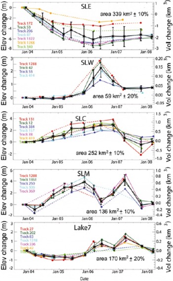
Fig. 3. Time series of estimated surface elevation and volume changes since October 2003 (Laser 2a) for the four main subglacial lakes (SLE, SLW, SLC, SLM) and lake 7. Coloured curves show the mean elevation and volume changes (elevation on the left-hand y axes, volume on the right) estimated from the individual ICESat tracks (see Fig. 1 for track locations); dashed curves indicate missing data, and tracks with no valid Laser 2a data are excluded. The thicker black curve is the weighted mean of all tracks; weights are equal to the lengths of the on-lake track segments. The error bars correspond to elevation; for volume they should be scaled by an additional 10% or 20%, depending on how the area was estimated.
Hydrologic regime 1
Subglacial Lake Engelhardt (SLE)
A large drainage event of SLE, between October 2003 and June 2006 (Fig. 4a), was reported by Reference Fricker, Scambos, Bindschadler and PadmanFricker and others (2007); here we also show the elevation anomalies associated with the repeats of ICESat track 53 along SLE, that were not included in our earlier paper (Fig. 4b). Image differencing presented in that study revealed the spatial extent of the drawdown for this lake, which we have re-estimated to be 339 km2 10% (cf. 350 km2 in the previous study). This area is sufficiently large that the ice above the lake is in hydrostatic equilibrium, as evidenced by the flat elevation profiles across it (Fig. 4a and b). The ice in this area is only ∼800 m thick (Reference Shabtaie and BentleyShabtaie and Bentley, 1988), and the lake length is ∼30 km (i.e. ∼38 ice thicknesses); therefore effects of ice-plate flexure at the edges have a minor effect on ice response to subglacial volume changes. This permits an accurate estimate of draining and filling rates from the observed surface deflation/inflation. The total volume of water released during the 2003–06 flood was estimated at 2.0 km3. SLE is located just ∼7 km upstream from the ice-shelf grounding line, and therefore its floodwater almost certainly discharges directly into the sub-ice-shelf cavity. Since June 2006, SLE has steadily filled at a rate of ∼0.4 m a−1 (0.14 km3 a−1) (Fig. 4a and b; see time series for tracks 53, 87, 206 and 1322 in Fig. 3).
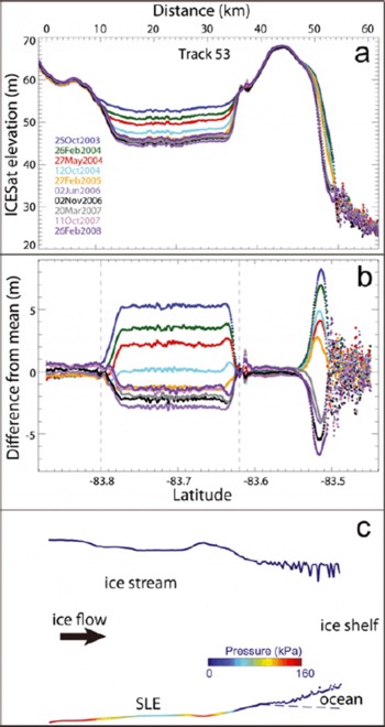
Fig. 4. Hydrologic regime 1. (a) Repeat ICESat elevation profiles along track 53, which crosses SLE and the grounding zone downstream, showing: (i) lake drainage from October 2003 through June 2006 (Reference Fricker, Scambos, Bindschadler and PadmanFricker and others, 2007) followed by filling through March 2008; and (ii) retreat of the grounding zone. The pass for 3 March 2006 (Laser 3e) that was shown in Reference Fricker, Scambos, Bindschadler and PadmanFricker and others (2007) has been omitted since the data across the grounding zone are invalid. (b) Elevation anomalies for track 53 repeats (not previously published). The anomaly plot reveals a flexure portion at the lake edges (similar to an ice-shelf grounding zone; Padman and Fricker, 2006) and flat portion in the centre. Vertical lines correspond to the limits of the elevation anomaly used to calculate the average elevation for each track at each campaign epoch. (c) Schematic cross-section through SLE with surface elevation from ICESat track 425 and bottom topography from our ice-thickness map (derived from Reference Shabtaie and BentleyShabtaie and Bentley, 1988). Vertical exaggeration is four times greater for the surface than for the base. The base is colour-coded by hydrostatic pressure from the hydrostatic-potential map in Figure 2.
Lake fill/drain cycles lead to changes in the ice-stream basal shear stress over the area of the lake, and this change could cause the ice surface to move vertically independent of water-volume changes (Reference Sergienko, MacAyeal and BindschadlerSergienko and others, 2007). In particular, the transitions across the lake edges should lead to ice extension and thinning upstream (transition to zero basal stress) and the opposite effects downstream (as ice regrounds). Because of its large size, large vertical elevation change and rapid discharge, we considered SLE the ideal case for observing the effects described in the Reference Sergienko, MacAyeal and BindschadlerSergienko and others (2007) study. Examining the elevation anomalies (Fig. 4b), we see that the October 2004 pass (L3a; cyan line in Fig. 4b) does show a couplet of ∼0.4 m elevation anomalies upstream and downstream on SLE. This pass was acquired during the period of maximum elevation change (maximum drainage rate, and presumably maximum grounding line shift). We interpret the elevation anomalies as a response of the ice to the shift in grounding location. The scale of the elevation change is an indication of the magnitude of the effect, i.e. an indication of the change in basal shear from ungrounded to grounded. We note that the width of the anomaly is ∼2 km (2.5 ice thicknesses), i.e. small with respect to the size of the lake. Thus we infer the majority of vertical movement over SLE is due to water volume change, and not ice dynamics; and in general, large subglacial lake activity (when the lake feature is several ice thicknesses across) should have volume changes dominated by water movement. Only when lakes are small relative to ice thickness, and in areas of high basal shear stress, would ice-dynamic effects dominate.
To aid understanding of SLE, we have produced a line schematic, along a profile through the lake and overlying ice, using ICESat surface elevation, ice thickness interpolated from our ice-thickness map (Reference Shabtaie and BentleyShabtaie and Bentley, 1988), and hydrostatic potential interpolated from the distribution presented in Figure 2 (Fig. 4c). ICESat track 425 crosses SLE almost exactly along-flow, and is nearly centered on the narrow zone downstream where the outlet channel for the lake is suspected. Because this track was acquired within hours of the end of a 33 day campaign (and the campaign terminations vary by a few hours) it has only been acquired twice, during Laser 2c and 3a (Fig. 1 for track location). The SLE schematic (Fig. 4c) shows its location with respect to the grounding line. The average hydrostatic pressure for SLE is ∼64 kPa and at the seal it is ∼128 kPa (relative to the potential pressure at the adjacent grounding line). The steady migration of Engelhardt Ice Ridge reported by Reference Fricker, Scambos, Bindschadler and PadmanFricker and others (2007) has continued and is visible in the ICESat data (Fig. 4b near 83.5° S). It remains an open question whether the grounding line in this region is migrating because of the lake, or whether the grounding line triggered retreat lake drainage.
Hydrologic regime 2
Subglacial Lake Whillans (SLW)
Reference Fricker, Scambos, Bindschadler and PadmanFricker and others (2007) inferred from ice surface elevation change that SLW had just filled in June 2006, after at least 2.5 years of inactivity. The additional data since June 2006 show that the maximum ice surface elevation over the lake was in June 2006 (Laser 3f) and was followed by a decrease of surface elevation over the next two ICESat campaigns (Laser 3g and 3h; Fig. 5a and b). This suggests that the residence time for the additional water was short ( ∼7 months). After that time, the ice surface elevation above the lake was about 0.5 m above the value it had maintained for more than 2 years preceding the filling event (October 2003 to November 2005). We estimate the total lake area from the MOA image combined with the limits from ICESat elevation anomalies to be 59 km2 ± 20%. The total estimated volumes of water SLW received during the filling event, and lost during the subsequent drainage event, are ∼0.13 and ∼0.09 km3 respectively.

Fig. 5. Hydrologic regime 2. (a) Repeat ICESat elevation profiles (upper plot) and elevation anomalies (bottom plot) for track 42 across SLW (see Fig. 1 for location). Vertical lines correspond to the limits of the elevation anomaly used to calculate the average elevation for each track at each campaign epoch. (b) Time series of estimated volume changes since October 2003 (Laser 2a) for SLW and lakes 10 and 12; dashed curves indicate data gaps. (c) Repeat ICESat elevation profiles for track 83 across lake 10 (see Fig. 1 for location).
Lake 10
Lake 10 is ∼35 km downstream of SLW and is approximately down-gradient (i.e. along a water flowline) in hydrostatic pressure. The surface elevation at this lake has continually risen throughout the ICESat period (Fig. 5b and c). The area of lake 10 is difficult to establish, but from the MOA combined with the limits of the ICESat elevation anomalies we estimate its area to be ∼25 km2 (± 20%). There is an increase in surface elevation after the SLW drainage event, but this appears to be at nearly the same rate as prior to that event. Given the small volumes associated with lake 10, it is difficult to tell conclusively whether it is linked to SLW.
Ice raft ‘a’
Immediately downstream of lake 10 is ice raft ‘a’ (Reference Shabtaie and BentleyShabtaie and Bentley, 1987a,Reference Shabtaie and Bentleyb; Reference AlleyAlley, 1993; Fig. 1), a region of thicker ice moving at the local rate of ice flow. Flow striping surrounding ice raft ‘a’ implies that at least at one stage it was stationary, and the surrounding ice flowed around it. The feature has recently been proposed as a source for icequakes observed in seismograms and the stick–slip nucleating point for a complex subglacial response to tidal forcing over a large region of the Whillans–Mercer ice plain (Reference Wiens, Anandakrishnan, Wineberry and KingWiens and others, 2008).
Across the downstream face of ice raft ‘a’, the ICESat repeats for track 83 (Fig. 5c; see Fig. 1 for location) show an elevation pattern consistent with an upstream migration of the bump, much like the grounding line retreat we observed at Engelhardt Ice Ridge (Fig. 4a). A similar signal (migration of the bump upstream) is also present on two tracks that intersect track 83 at ice raft ‘a’ (tracks 191 and 310; see Fig. 1 for location). Additionally, the ICESat repeats across the surface bump associated with ice raft ‘a’ fall into two sets of curves, whose peaks are aligned at two locations, and there is a jump in the peak location upstream, from one peak location to the other, at the same time as the arrival of the SLW water at lake 10, followed by steady continuous migration upstream (Laser 3g to Laser 3i to Laser 3j), i.e. constant upstream migration of bump, but punctuated with faster migration coinciding with arrival of water in the lake. This suggests that the lake filling affects the ice dynamics. There is also some evidence of a dipole in the difference plots, similar to that shown by Reference Sergienko, MacAyeal and BindschadlerSergienko and others (2007). It is possible that we are observing stick–slip motion (Reference Bindschadler, King, Alley, Anandakrishnan and PadmanBindschadler and others, 2003), but aliased by the ICESat temporal sampling. Whatever the cause, it seems to be the case that ice raft ‘a’ has a complex interaction with the ice-stream bed, possibly moderated by subglacial water flow.
Lake 12
Lake 12 is the most downstream lake in regime 2 (Figs 1 and 2), and its drainage event was documented by Reference Fricker, Scambos, Bindschadler and PadmanFricker and others (2007). An elevation decrease of approximately 1.5 m was observed on both ICESat tracks between November 2003 and March 2006. From MOA combined with ICESat elevation anomaly limits on two intersecting tracks, we estimate its area to be 64 km2 (±20%). The volume of water lost by the drainage event was ∼0.08 km3; the lake filled by ∼80% of that volume amount soon after SLW drained (Fig. 5b). It appears that floodwater from SLW goes primarily to lake 12, with some possibly also going to lake 10.
Hydrologic regime 3
Subglacial Lake Conway (SLC)
The ice surface elevation across SLC started to decrease sometime between June 2006 (L3f) and November 2006 (L3g), which we interpret as a flooding event (Fig. 6a). New image-differencing results over the region surrounding SLC (2007–05; Fig. 6b) confirm that the lake subsided over that time period and provide the spatial extent of the subsidence area; from this image we estimate the SLC area to be 252 km2 (± 10%). The magnitude of subsidence varied across the lake, with the largest elevation anomalies occurring in the south. This was a significant flooding event involving a large amount of water (∼0.83 km3) that persisted until November 2007.

Fig. 6. Hydrologic regime 3. (a) Repeat ICESat elevation profiles (upper plot) and elevation anomalies (bottom plot) for track 131 across SLC (see Fig. 1 for location). Vertical lines correspond to the limits of the elevation anomaly used to calculate the average elevation for each track at each campaign epoch. (b) Difference image for the period November 2007–November 2005 over the three lakes. ICESat track segments are colour-coded by the elevation decrease over approximately the same period. (c) Repeat ICESat elevation profiles (upper plot) and elevation anomalies (bottom plot) for track 8 across USLC (see Fig. 1 for location). (d) Repeat ICESat elevation profiles (upper plot) and elevation anomalies (bottom plot) for track 1351 across SLM (see Fig. 1 for location). (e) Hydrostatic potential along a line spanning the three lakes (see white dashed line in (b) for location). (f) Time series of estimated volume changes since October 2003 (Laser 2a) for USLC, SLC and SLM; vertical dashed lines show the epochs used for the image difference in (b).
Upper lobe of SLC
The hydrostatic-potential map (Fig. 2) revealed a hydrologically flat region ∼10 km upstream of SLC. The hydrostatic potential pressure of this upper region is approximately 200 kPa greater than that of the center of SLC. ICESat tracks in the area provide evidence of an active lake, which appears to be draining with a maximum surface elevation decrease of ∼2–3 m over the period 2003–08 (Fig. 6c). ICESat data over this lake are noisy due to intense surface crevassing, which makes estimates of timing and volume difficult, but the elevation decrease there appears to have started several months prior to SLC, albeit at a much smaller amplitude. We consider this an ‘upper lobe’ of SLC, and hereafter refer to it as USLC. It seems likely that the drainage of SLC was triggered in part by the receipt of floodwater from USLC. Since the surface deformation of USLC is indiscernible in the difference image (Fig. 6b), we estimate its surface area (177 km2 ± 20%) from the limits of the elevation-change signal observed on seven ICESat tracks and co-located surface features in MOA. The estimated volume of water expelled during the USLC flooding event is ∼0.34 km3 (0.24 km3 between June 2006 and November 2007), giving a total of 1.07 km3 for the combined USLC/SLC flooding event.
Subglacial Lake Mercer (SLM)
The surface elevation of SLM increased steadily from October 2003 until November 2005 (Laser 3d), then decreased steadily until June 2006 (Laser 3f), which has been interpreted as a drainage event (Reference Fricker, Scambos, Bindschadler and PadmanFricker and others, 2007; Fig. 6d). Track 116 does not have data in either Figure 1 or Figure 6b because of large deviations from the reference track, including off-pointing in November 2005. From the difference image (Fig. 6b) we re-estimate the area of SLM to be 136 km2 ± 10% (cf. 120 km2 by Reference Fricker, Scambos, Bindschadler and PadmanFricker and others (2007) based solely on MOA). The total amount of water lost by the flooding event was ∼0.45 km3. After June 2006, the elevation increased until February 2007; after that it decreased again. We interpret this as a secondary drainage event for SLM, discharging ∼0.58 km3, and believe it to be related to the drainage of SLC upstream.
USLC/SLC/SLM link
The ICESat-derived surface displacements are consistent with water movement occurring between USLC, SLC and SLM, suggesting that they are connected. A profile taken from the new hydrostatic-potential map along the USLC, through SLC and then through SLM shows the pressure gradient among the lakes along a line of minimum hydrostatic potential connecting the three, i.e. the likely path of water flow between them (Fig. 6e; see Fig. 6b for location). USLC has a hydrostatic potential pressure 230 kPa higher than SLC, and SLC in turn has ∼240 kPa higher pressure than SLM. All three lakes are located in well-defined hydrostatic potential minima. We note that the hydrostatic potential (or hydraulic head) is not completely flat on the lakes themselves, and therefore these lakes would not pass one of Reference Carter, Blankenship, Peters, Young, Holt and MorseCarter and others’ (2007) criteria for a lake. The surface elevation of SLM is 100 m, ∼50 m above the surface elevation of the grounding line. There is a pressure barrier in between the lakes that is presumably breached when SLC drains; however, the outlet conduit is too small to be resolved at this scale. Figure 2 suggests that the most probable pathway for subglacial water from SLC towards the ocean would be through SLM.
The hydrologic link between SLC and SLM is also apparent from the time-series plot of volume change of both lakes (plus USLC) for 2003–08 (Fig. 6f). From this plot, we infer that the floodwater from SLC is directed to SLM: in the time that SLC lost ∼0.5 km3 of water (i.e. between June 2006 and March 2007), SLM gained ∼0.45 km3. The lake volume threshold (i.e. the full capacity of the lake just before it drains) appears to be about ∼0.5 km3 greater than its volume immediately after flooding. At around the time when water from SLC started to reach SLM (June 2006), SLM had just drained. When the capacity of SLM had increased by ∼0.5 km3 again (March 2007), the lake was full again and started to drain. We propose that, once the outlet conduit for SLM was open, the additional floodwater arriving from SLC moved directly through SLM (the outlet was hydraulically jacked open, i.e. the subglacial water pressure exceeded the ice overburden pressure). This is similar to the scenario that was recently proposed to have occurred at the Adventure Trench lakes (Carter and others, in press). During that flooding event, discharge from lake U2 likely passed straight through lake U3, since U3 was already full and the additional water entering it overflowed.
Downstream of SLM
The floodwater from the USLC/SLC/SLM flood appears to have arrived at two locations down the hydrostatic potential gradient from SLM (lakes 7 and 8; Fig. 1) at around the same time (although accurate timing is not possible due to the coarse temporal sampling of ICESat), and temporarily ponds in these regions. Lake 7 is larger than originally suggested by Reference Fricker, Scambos, Bindschadler and PadmanFricker and others (2007) and appears to be joined to their lake 9. This inferred large water body is contained within a distinct trough associated with flowband in the Mercer/Whillans Ice Stream suture zone that is clearly visible in MOA. The hydrostatic potential is constant ( ∼28 kPa) along this entire elongated feature, and the surface elevation is 65–70 m; the estimated area from MOA combined with ICESat elevation-change limits is ∼170 km2 (±20%). Repeat elevation profiles for ICESat track 27 across this trough are shown in Figure 7a. Lake 8 is a smaller lake (area from MOA is ∼52 km2 ±20%) that sits at a slightly higher hydrostatic potential (∼30 kPa; surface elevation 78 m).

Fig. 7. Hydrologic regime 3, downstream of SLM. (a) Repeat ICESat elevation profiles (upper plot) and elevation anomalies (bottom plot) for track 27 across lake 7 in the Mercer/Whillans Ice Stream paleo-suture zone (see Fig. 1 for location). Vertical lines correspond to the limits of the elevation anomaly used to calculate the average elevation for each track at each campaign epoch. (b) Time series of estimated volume changes since October 2003 (Laser 2a) for lakes 7 and 8. Peaks 1 and 2 correspond to the arrival of USLC/SLC/SLM floodwater at the lakes, as discussed in the text.
Lake 7 appears to have received the majority of the floodwater, although the residence time for the water there was short (approximately March–June 2006). It appears that some floodwater also went to lake 8, whose activity matched that of lake 7, i.e. the surface elevations at this lake are in phase with those at lake 7 (Fig. 7b) but at much lower amplitude. The ICESat tracks across lake 7 that have no coloured segments in Figure 1 had no valid repeats when the lake was full. The timings of the peaks of the time series for lakes 7 and 8 (Fig. 7b) are consistent with these regions receiving water from the flooding of SLM (peak 1) and SLC/SLM (peak 2).
5. Comparison of Subglacial Activity for Mercer/Whillans Lakes
5.1. Short-term activity (days to weeks)
In our earlier study (Reference Fricker, Scambos, Bindschadler and PadmanFricker and others, 2007), we noted that the detected elevation-change regions displayed a variety of temporal signatures, and that changes occur on short timescales (e.g. between two ICESat campaigns). We considered whether lake levels might fluctuate on timescales shorter than the ICESat sampling; if this is the case, our time series would be aliased plots of the true lake activity. However, we note that for the larger lakes (see, e.g., the time series for SLM; Fig. 3) there are several ICESat tracks across the lake on different days within the 33 day laser campaign. If there was lake activity on the sub-daily or even sub-monthly timescale, we would expect to see variability in the lake states from the different acquisition times of tracks within the campaigns. Since we do not see this, we believe that the lake states are similar for each pass within the same ICESat campaign, and that it is unlikely that there is any significant short-term activity going on within or between these 33 day periods.
5.2. Long-term activity (months to years)
Over the observation period of our previous study (October 2003–July 2006), SLE, SLC and SLM showed constant activity between each ICESat campaign, whereas SLW showed periods of quiescence. The additional four ICESat campaigns since that study provide us with a 4.5 year time series (October 2003–March 2008). While this length of time is insufficient to quantify exact periodicity for our lakes, it enables us to begin to identify patterns in subglacial lake activity and to make preliminary comparisons between lakes.
Returning to the time series for the five main lakes on Mercer/Whillans (Fig. 3), we note that there are distinct categories; however, we note that the overall length of the ICESat data record is still short relative to the apparent periodicity of each lake. SLE and SLC are located in the ice-stream shear margins, close to ice ridges, and have long-period (of order decades) steady filling/draining cycles, and larger water volumes involved in the cycle. SLM has a similar pattern to these two lakes, but the period is shorter (of order 2–3 years) and its cycle is complicated by the fact that this lake also receives floodwater from SLC. SLW and lake 7 are located under the ice stream proper and have a shorter period; the additional water entering these lakes has a short residence time, i.e. a filling event is soon followed by a drainage event. These lakes only received single pulses of water during this period, and the water had relatively short residence times (∼1year). There also appears to be a correlation between lake size and fill/drain event periodicity. Larger lakes within the Whillans–Mercer system (SLE, SLC and SLM) have a longer cycle between fill and drain events; smaller lakes such as SLW and lakes 7, 8 and 10 have more frequent, or rapid, events. If we assume that lake volume generally scales with lake area, this is consistent with the requirements of a connected flow system transporting a given flux of water through a series of reservoirs. A similar observation was made for subglacial outburst floods from lakes in the Tien Shan, central Asia; smaller lakes (smaller relative to the annual melt flux in their catchments) had more frequent outbursts; larger lakes had less frequent floods (Ng and Liu, in press).
6. Effect of Lakes on Ice Dynamics
Ice-stream subglacial hydrology is a key process at the basal ice-sheet boundary that needs to be understood before it can be reliably incorporated into ice-sheet models and assessments of future sea-level rise. This is important because the presence of water under an ice stream, and the concomitant change in basal stress, must affect how fast it flows. The discovery of active subglacial systems provides a mechanism whereby basal lubrication conditions, and therefore discharge rates, can alter much more rapidly than previously thought; this realization has forced us to rethink the timescales on which ice streams change (Reference Truffer and FahnestockTruffer and Fahnestock, 2007; Reference Vaughan and ArthernVaughan and Arthern, 2007). The suspected link between subglacial lakes and ice dynamics has recently been confirmed by observations at Byrd Glacier, where flooding of two large lakes upstream caused a 10% speed-up of the glacier trunk, sustained for ∼14 months (Reference FrickerFricker, 2008; Reference Stearns, Smith and HamiltonStearns and others, 2008).
There are still several open questions related to sub-ice-stream lakes: (1) what is the effect of the lakes on the rest of the ice-stream subglacial water system? (2) how do flooding events affect ice dynamics? (3) do the lakes completely empty when they drain? A lake drainage event initiates when the hydrostatic pressure in the lake has increased to a point that the pressure barrier at the downstream seal is breached. A flood from a lake acts to reduce this pressure back to equilibrium level. Once equilibrium is reached, the flood stops. There is no reason to assume that this means the lake is now empty. Therefore we believe that, in general, it is not the presence of the lakes themselves that perturbs the ice motion, but the transfer of water between the lakes. It is difficult to test this hypothesis, as there are no InSAR data over the lakes coinciding with the ICESat period, and the region discussed here is too far south for much higher-resolution visible-band image data for velocity mapping. In the absence of simultaneous velocity data over the Mercer and Whillans Ice Streams, it is not possible to determine whether the flooding events documented here affected ice velocities. The link between lakes and ice dynamics is being investigated during ongoing fieldwork in the region during the 2007/08 and 2008/09 Antarctic field seasons (Reference Tulaczyk, Pettersson, Quintana-Krupinski, Fricker, Joughin and SmithTulaczyk and others, 2008). In the future, data from ICESat-II (currently planned for launch in 2015) or other elevation satellite or airborne missions, combined with coincident velocity measurements, would provide much-needed information towards understanding the link between the subglacial system and ice dynamics.
7. Conclusions
We have examined the activity of the subglacial water system beneath lower Mercer and Whillans Ice Streams for the period October 2003–March 2008 using ICESat repeat-track analysis and satellite image differencing. Since 1 January 2007, the temporal sampling of the ICESat data has reduced to twice a year, but the most recent data have revealed important new information about this subglacial water system. Several significant events took place during that time. The most noteworthy event was the drainage of USLC/SLC since June 2006, discharging an estimated 0.86 km3 of water. ICESat analyses suggest that some of this water was directed to SLM; while SLC was draining, SLM filled and then drained, strongly suggesting that these two lakes are connected hydrologically. Water from this flood was channeled downstream towards the ocean along a surface depression lying along the suture zone between Mercer and Whillans Ice Streams, and pooled there temporarily. The locations of these downstream signals correspond to depressions in the surface topography that are also visible in the MOA image of the region. SLW also appears to be linked to the next region down the hydrostatic potential gradient in its regime. Our analysis also looked at SLW and subglacial activity near ice raft ‘a’ (Reference AlleyAlley, 1993), a prominent feature of the ice plain of Whillans Ice Stream. Inferred hydrologic activity, marginal changes akin to grounding-line retreat, and results of other studies showing that the ice raft is a locus of stick–slip activity over a large portion of the ice plain (Reference Wiens, Anandakrishnan, Wineberry and KingWiens and others, 2008) all point to this feature having a complex interaction with the ice-plain bed.
With the 5 year time-span of ICESat data, we are now able to investigate the activity cycles of the lakes in this system, although the time series is still short relative to the apparent periodicity of the lakes. We notice distinct patterns in lake activity: larger lakes located next to ice-stream shear margins have long, steady fill/drain cycles; whereas smaller lakes under the faster-flowing parts of the ice stream have shorter cycles and short residence times for the additional water. We believe that the frequency of outburst flood events is related to subglacial water supply and lake capacity, but may involve other factors such as: basal lithology or till thickness; local bed and ice surface relief (e.g. the variability of the hydrostatic potential field); and, as we show here, the activity of lakes hydrologically upstream of a given subglacial reservoir.
Acknowledgements
We thank B. Smith, S. O’Neel and R. Radpour for help with the ICESat data interpretation. We also thank T. Haran for help with the MODIS image differencing and hydrostatic-potential mapping, and S. Carter for providing his SLM outline. We thank NASA’s ICESat Science Project for distribution of the ICESat data (see http://icesat.gsfc.nasa.gov and http://nsidc.org/data/icesat). We thank R. Bingham, N. Glasser and an anonymous reviewer for thorough reviewing, which greatly improved the paper. H.A.F. was supported by NASA grant NNX07AL18G.


