


1. Introduction
1.1 Glacial hydrology
Glacial ice flow needs to be understood to project future sea level rise precisely. Ice flow occurs by either internal ice deformation or basal motion, which is influenced by the subglacial hydraulic system (e.g. Iken and others, Reference Iken, Röthlisberger, Flotron and Haeberli1983; Kamb, Reference Kamb1987; Bartholomaus and others, Reference Bartholomaus, Anderson and Anderson2008; Bartholomew and others, Reference Bartholomew2010; Andrews and others, Reference Andrews2014). Just before the onset of the melt season, basal water resides in a distributed system of cavities. When surficial meltwater inputs to the bed increase, the amount of water in the cavity system increases, overwhelming narrow wintertime channels and cavities, and the glacier is raised off the bed, increasing sliding (e.g. Iken and others, Reference Iken, Röthlisberger, Flotron and Haeberli1983; Iken and Truffer, Reference Iken and Truffe1997; Sugiyama and Gudmundsson, Reference Sugiyama and Gudmundsson2004; Gräff and others, Reference Gräff, Walter and Lipovsky2019). With continuing high water supply into the mid melt-season, channels are incised into the bed or melted into the overlying ice, depending on basal conditions, widening them and efficiently transporting water through the subglacial environment to the glacier terminus (e.g. Kamb, Reference Kamb1987; Fountain and Walter, Reference Fountain and Walder1998). Well-developed channel systems lower water pressures and thus increase effective pressure, the difference between ice and water pressure (e.g. Röthlisberger, Reference Röthlisberger1972), thereby increasing basal contact area and friction and decreasing basal sliding (e.g. Iken, Reference Iken1981; Iken and others, Reference Iken, Röthlisberger, Flotron and Haeberli1983). Low water pressure is maintained by melting of channel walls by the heat generated by viscous dissipation in the flowing water. At the end of the melt season, surface meltwater inputs to the bed decrease and channels experience creep-closure to ‘reset’ the majority of the hydraulic system to a high-water-pressure distributed wintertime system (e.g. Kamb, Reference Kamb1987; Fountain and Walder, Reference Fountain and Walder1998).
Glacial hydrology has been studied for decades, but many of the prior methods (e.g. boreholes, tracers, active geophysics) have been limited to point measurements or short time windows, inhibited by hundreds of meters of overlying ice, the difficulty of maintaining on-ice instruments through seasonal ablation/accumulation, and other challenges. Water moving through englacial or subglacial channels generates continuous seismic signals known as glacial hydraulic tremor (GHT) that can be distinguished from other sources (e.g. Sergeant and others, Reference Sergeant2020). GHT can be monitored with seismometers located on glacier marginal bedrock, and can be used to study the spatiotemporal evolution of the glacial hydraulic system continuously and remotely. It can provide important information on basal water pressure changes, subglacial discharge channel sizes, sediment transport (Bartholomaus and others, Reference Bartholomaus2015; Gimbert and others, Reference Gimbert, Tsai, Amundson, Bartholomaus and Walter2016; Nanni and others, Reference Nanni2020; Lindner and others, Reference Lindner, Walter, Laske and Gimbert2020) and location and distribution of channels beneath the ice (Winberry and others, Reference Winberry, Anandakrishnan, Alley, Bindschadler and King2009; Aso and others, Reference Aso2017; Vore and others, Reference Vore, Bartholomaus, Winberry, Walter and Amundson2019). Various frequency ranges within GHT have been associated with subglacial and englacial turbulent water flow (e.g. Bartholomaus and others, Reference Bartholomaus2015; Gimbert and others, Reference Gimbert, Tsai, Amundson, Bartholomaus and Walter2016; Vore and others, Reference Vore, Bartholomaus, Winberry, Walter and Amundson2019) and bedload transport (Gimbert and others, Reference Gimbert, Tsai, Amundson, Bartholomaus and Walter2016, Reference Gimbert, Fuller, Lamb, Tsai and Johnson2019).
1.2 Study site and previous studies
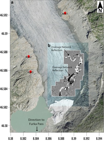
In this study, two years (2018 and 2019) of passive seismic data collected from three ice-proximal bedrock-based seismic stations deployed at Rhonegletscher, Switzerland (Fig. 1) are assessed for GHT. We calculate back azimuth angles to tremor sources according to the methods of Vore and others (Reference Vore, Bartholomaus, Winberry, Walter and Amundson2019), and inspect for power–discharge relationships as identified by Gimbert and others (Reference Gimbert, Tsai, Amundson, Bartholomaus and Walter2016, Reference Gimbert, Fuller, Lamb, Tsai and Johnson2019) and Nanni and others (Reference Nanni2020). Rhonegletscher, in the central Swiss Alps, is ~9 km long, flowing south from an elevation of 3600–2200 m above sea level (GLAMOS, 2018). It is one of the most extensively studied glaciers in the world, with the earliest scientific observations in 1874 (Mercanton, Reference Mercanton1916).

Fig. 1. (A) Map location of the bedrock-based seismic stations used in this study. (B) GPR location of the channel from Church and others (Reference Church, Bauder, Grab and Maurer2021) Supplementary Materials at elevation slices between 2215 and 2210 m above mean sea level.
A similar seismic study (Canassy and others, Reference Canassy, Röösli and Walter2016) inspected seismic data on Rhonegletscher for hydraulic tremor over 2012 and 2013. Our study builds on this prior work by providing a continuous record over a similar time span of two years (2018 and 2019), but with fewer seasonal data gaps than in Canassy and others (Reference Canassy, Röösli and Walter2016). They observed an increase in persistent seismic energy during the melt season concentrated below 10 Hz during 2012 and 2013. Canassy and others (Reference Canassy, Röösli and Walter2016) attributed some of the summer seismic energy to increased englacial tensile fracture events, driven by increased ice flow, in agreement with prior work (Neave and Savage, Reference Neave and Savage1970; Roux and others Reference Roux, Marsan, Métaxian, O'Brien and Moreau2008; Mikesell and others Reference Mikesell2012; Röösli and others Reference Röösli2014). However, they concluded that because such fracture events typically generate energy in the range 10–100 Hz, fracture events alone likely do not account for the high seismic energy concentrated at lower frequencies (<10 Hz), the rest being explained as water-flow-induced tremor.
A water-filled channel alternating spatially between a subglacial and englacial location was imaged using reflection seismic profiling in 2012 and 2017, and also using repeated 2D ground-penetrating radar (GPR) several times in the winter and summer of 2018 and winter of 2019 (Church and others, Reference Church2019), and 3D GPR in 2020 (Church and others, Reference Church, Bauder, Grab and Maurer2021). During the melt seasons of 2018, 2019 and 2020, the vertical channel extent was estimated to be ~0.2–0.4 m and the channel width 8–25 m, increasing downstream. Thickness of the channel throughout the study region was at the limit of the radar resolution (<0.4 m), and thus thickness changes spatially could not be discerned. Boreholes drilled into the channel during July 2018 found generally stable water levels with occasional short, abrupt increases. Church and others (Reference Church2019) observed fast-flowing water in the channel laden with suspended sediment and immobile gravels, and inferred that the channel is fed by upstream supraglacial meltwater and by morainal streams that dive under the glacier where the ice and moraine meet.
2. Methods
2.1 Frequency-dependent polarization analysis
We used frequency-dependent polarization analysis (FDPA; Park and others, Reference Park, Vernon and Lindberg1987) to identify bands of locatable (polarized Rayleigh wave) tremor within the overall signal of GHT on Rhonegletscher, Switzerland, and assess the temporal and spatial extent of these bands. The use of FDPA to study GHT was previously developed for and applied on Taku Glacier, Alaska, by Vore and others (Reference Vore, Bartholomaus, Winberry, Walter and Amundson2019). We closely follow their methods, with slight modifications, using three ice-proximal bedrock-based seismic stations (Fig. 1; RA41, RA42 and RA43) around Rhonegletscher, each composed of a three-component Lennartz LE-3D/5s seismometer with a natural frequency of 0.2 Hz and sampled at a rate of 200 Hz. The following is a brief description of how the data were processed. A more detailed description on how GHT was classified and assessed is included in the Supplementary Materials (S1), and we direct readers to Vore and others (Reference Vore, Bartholomaus, Winberry, Walter and Amundson2019) method section 3.1.1 for further elaboration.
The seismic data were windowed into 7 min segments, and then a singular value decomposition was performed on the averaged spectral covariance matrices (the Fast Fourier Transform (FFT) multiplied by its conjugate) at each station. The decomposition extracted information on seismic energy, degree of polarization, amplitude and phase for signals in a specified frequency range. These data allowed us to characterize GHT on Rhonegletscher in terms of power, polarization and wave type. We determined thresholds (explained in the Supplementary Fig. S1) for each of these quantities to distinguish signals of locatable GHT from non-locatable GHT and ambient noise sources. Studies of GHT generally focus on frequencies between 1 and 10 Hz to isolate signals from turbulent water flow (e.g. Bartholomaus and others, Reference Bartholomaus2015; Vore and others, Reference Vore, Bartholomaus, Winberry, Walter and Amundson2019); some studies also analyze 10–20 Hz to isolate signals from transport of coarse-grained sediment (e.g. Hsu and others, Reference Hsu, Finnegan and Brodsky2011; Burtin and others, Reference Burtin2011; Schmandt and others, Reference Schmandt, Aster, Scherler, Tsai and Karlstrom2013; Gimbert and others, Reference Gimbert, Tsai, Amundson, Bartholomaus and Walter2016). In this study, we calculated the median power spectral densities from 1.5 to 10 Hz to capture signals from turbulent water flow and exclude signals that dominate between 1 and 1.5 Hz (e.g. Vore and others, Reference Vore, Bartholomaus, Winberry, Walter and Amundson2019; Bartholomaus and others, Reference Bartholomaus2015). Signals from higher frequencies (>10 Hz) are deferred for future studies, which would benefit from additional work monitoring water pressure and sediment transport from within the channel along-side a seismic analysis.
2.2 Determining back azimuth angle
Using the information on wave type, any frequencies coming from a source with consistent phase lag between the horizontal and vertical components of the waveform can have a back azimuth angle Ѳ calculated using a relation between the amplitude of motion in the two horizontal directions (A E for east west and A N for north-south) obtained from the polarization vector P o (see Supplementary Materials; e.g. Haubrich and others, Reference Haubrich, Munk and Snodgrass1963; Takagi and others, Reference Takagi, Nishida, Maeda and Obara2018; Vore and others, Reference Vore, Bartholomaus, Winberry, Walter and Amundson2019). That is, any frequencies with substantial polarized Rayleigh wave composition can have a back azimuth angle toward the source estimated according to (1):

While we observed many consistently high-power frequency bands during the melt season related to hydraulic activity with a large degree of Rayleigh waves present, we will focus our discussion of back azimuths specifically on those identified as polarized Rayleigh waves that exceed our power threshold (Supplementary Materials S1.1).
2.3 Discharge and weather data
We compare our findings with meteorological data from a MeteoSwiss station in Grimsel Hospiz located ~4 km west of Rhonegletscher behind a mountain ridge at an elevation of 1980 m.a.s.l. We use stream-discharge data from station 2268 in Gletsch managed by the Swiss Federal Office for the Environment (BAFU), located ~3 km downstream at 1756 m.a.s.l. During the melt season, ~90% of the measured stream discharge at Gletsch originates from Rhongletscher. It takes discharge from Rhonegletscher ~1–3 h to travel from the glacier to the location of the discharge station.
2.4 Power versus discharge relations
Relations between seismic power P and turbulent subglacial discharge Q have been developed for end-member behaviors of water channels by Gimbert and others (Reference Gimbert, Tsai and Lamb2014) (further explored in Gimbert and others (Reference Gimbert, Tsai, Amundson, Bartholomaus and Walter2016) and Nanni and others (Reference Nanni2020); also see Lindner and others (Reference Lindner, Walter, Laske and Gimbert2020); (2) and (3)). These are:


where P w is the total noise power spectral density for frequencies due to water channels with turbulent flow. Situations in which the power–discharge relation follows (2) is referred to as ‘variable pressure gradient’ and (3) as ‘constant pressure gradient’, in reference to whether the water pressure in the hydraulic system is variable and confined by a constant channel geometry (on the timescale of relevance), or if water pressure is held constant over time with fluctuations in water discharge accommodated by changes in channel geometry. In previous literature, the power versus discharge relations have been plotted after being scaled by a ‘reference’ value, typically chosen as the start of the record or at a time of minimal power and discharge (e.g. Gimbert and others, Reference Gimbert, Tsai, Amundson, Bartholomaus and Walter2016). We chose this reference as an arbitrary power–discharge pair from a time interval outside of the melt season during lower power and discharge (i.e. in January). How the power and discharge values are scaled by these references does not change the relationship and only affects the appearance of subsequent plots.
3. Results
3.1 Glacier hydraulic tremor frequency bands
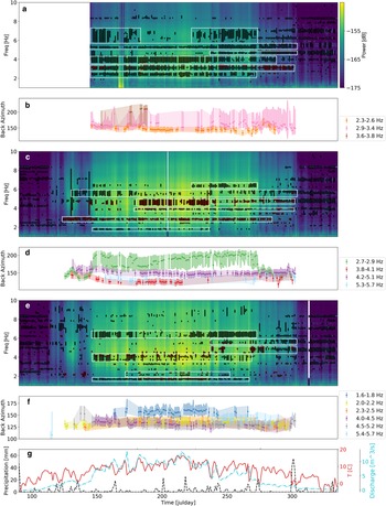
During late spring, summer and early fall, the median power spectra of the seismic station display a noticeable increase in background power relative to the quiescence of the winter months (Figs 2, 3A, C, E), which is related to increases in water discharge (Figs 2, 3G). For our purposes, we define this period of high median power as the melt season. In the winter, the power threshold (Supplementary Materials S1.1) is surpassed in many frequency bands (black dots indicating a power peak in Figs 2, 3A, C, E that occur earlier than day 100 and after day 300 of the year). Lower overall median seismic power in winter allows small peaks in power to appear more prominent, causing the detection of power peaks throughout the winter, despite relatively little hydrological activity compared to the summer. In summer, many of the winter bands cease or are weaker than the signal related to water flow during the melt season, and spectral bands related to subglacial and englacial water are more prevalent.

Fig. 2. Results for 2018 are plotted from 1 April to 1 December for stations RA41, RA42 and RA43. Plots A, C and E show the median power spectra for the frequencies 1.5–10 Hz. Black dots overtop the spectra indicate days when the power threshold (Supplementary Materials S1.1) was surpassed. A red outline of a black dot indicates that the FDPA analysis identified locatable GHT. Boxes are drawn around frequency bands identified as related to subglacial and englacial water flow. If an outlining box is colored, at least part of the enclosed frequency band was identified by FDPA as polarized Rayleigh waves and has a corresponding back azimuth angle calculation plotted over time in the same color as the outlining box in the following plots. Plots B, D and F depict the back azimuth angles calculated per each frequency band of GHT detected each day. The shading indicates the interquartile range, and the dot the median value of the back azimuth angle. Plot G shows the mean daily temperature and precipitation from a nearby MeteoSwiss station, and discharge measured 3 km downstream of Rhonegletscher. Back azimuth bands and the boxes around bands in the median spectra plots use the same colors for the respective bands, with a white box representing a band that did not have any locatable GHT via FDPA analysis.

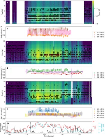
Fig. 3. Results for 2019 are plotted, following the same conventions as Figure 2.
We focus on summer bands that were active for at least several consecutive days at multiple times across a season. Seven main bands of tremor are identified visually between the three stations this way, and named for the general frequency (in Hertz) around which each is centered for ease of description in the text: 6, 5.5, 4.5, 4, 3, 2.5 and 1.7 Hz. Within these bands, the FDPA analysis identified frequencies of locatable Rayleigh wave GHT during the 2018 and 2019 melt seasons at all seismic stations. During the melt season, only Rayleigh waves, and no body/Love or mixed-type waves, meet the required wave-type threshold (e.g. Supplementary Fig. S2), indicating that primarily Rayleigh waves related to GHT are being identified in the range of 1.5–7 Hz. No significant GHT is found above 7 Hz, nor are Love waves, body- or mixed wave types detected at any frequency on Rhonegletscher. Bands spanning a similar range are present in both years, although the exact upper and lower bounds of some bands vary slightly.
In general, within each frequency band, the back azimuth is constrained to a narrow range that does not change much across seasons and years, with a few exceptions (Figs 2, 3B, D, F). To avoid misinterpreting non-glacial signals, the back azimuth angles of the detected frequency bands were compared with the back azimuth angle (per each station location) to the two most likely non-GHT sources of tremor: the waterfall draining the terminal lake at the glacier toe; and, the Furka Pass, a mountain road located near Rhonegletscher that is seasonally open for heavy tourism traffic. None of the back azimuth angles of the identified GHT bands consistently align with the back azimuth angle to the waterfall or lake. There is some overlap with the back azimuth angle of Furka Pass, but the high power in the frequency bands in question generally began earlier in the year than the opening date of the road, indicating power in these bands is being generated by a natural phenomenon related to the seasonal increase in median power and not to anthropogenic causes.
The duration and back azimuth angles of the power in the frequency bands of interest (Figs 2, 3B, D, F, 4) were also compared to regional air temperature, precipitation and discharge data (Figs 2, 3G). Before the melt season, discharge values remained at a low baselevel. Discharge gradually increased over the spring, and closely followed air temperature once the mean annual daily air temperatures remained consistently higher than ~5°C, indicating air temperature-driven glacier melt was the dominant source of water into the system. Individual precipitation events did not appear to have any long-term influence on back azimuth angle or duration of the power in the identified frequency bands. Peak temperatures occurred each day between 11:00 and 15:00 local time, depending on the time of year, with peak power in the 1.5–10 Hz range generally lagging peak temperature by 2–6 h. We interpret the ~1 h lag of peak discharge behind peak power as arising from the time for the water to flow from the glacier to the gauging station, and we correct for this offset by applying a 1 h shift before inspecting power–discharge relations (section 3.2).

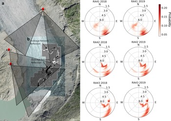
Fig. 4. Map of the stations (A) and known channel location in 2018 (B; Church and others, Reference Church, Bauder, Grab and Maurer2021). (C) Polar plots of back azimuth angles calculated for Rayleigh waves at each station in 2018 and 2019 for the frequency range of 1.5–6 Hz. The abundance of Rayleigh waves on Rhonegletscher accounts for the large number of back azimuth angles calculated across the frequency range; however, only those bands noted in Figures 2 and 3B, D, F were identified as GHT by the FDPA analysis. The color bar indicates the value of the probability density function plotted per each frequency bin on the polar plots, with darker red indicating a greater degree of probability per the angle. For example, 25 July is plotted for all years and stations, but similar values were observed across the entire melt season each year.
The identified frequency bands generally became active in the spring when daily discharge values surpassed ~5 m3 s–1. Part-way through the melt season, once discharge began to intermittently decrease below this value as daily temperature decreased, some bands displayed temporary shifts in back azimuth angle, turned on or off, or slightly shifted in frequency range. These changes first began to occur around 25 August (day 237) in 2018 and 6 September (day 249) in 2019 (Figs 2, 3). A more detailed description of the frequency bands per each station is included in the Supplementary Materials (S2).
3.2 Power–discharge relationships
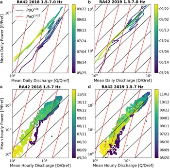
We inspected the seismic power between 1.5 and 7 Hz (where all of our detected tremor bands occur) versus the discharge data to compare trends in our data to the relations of (2) and (3). We focus on the interval from late May to early November to capture the full melt season from onset to end. We show the data from both years from Station RA42 in Figures 5–7; data from the other stations are consistent (Supplementary Fig. S3). We show full hourly resolution data for a time interval spanning the full melt season with a little extra time on each end, in Figures 5D and D. To more clearly highlight certain features, we use smooth lines for selected shorter melt-season-specific time intervals in Figures 6 and 7, and we display daily-average data with smooth lines in Figures 5A and B. These plots best capture the patterns we observed, showing that the power–discharge relations generally vary on a seasonal (Fig. 5) and diurnal (Fig. 6) scale, and exhibit abrupt changes during storms (Fig. 7).

Fig. 5. Plots of seasonal seismic power between 1.5 and 7 Hz versus discharge for station RA42. The discharge and power are scaled by a reference value (Q ref and P ref, respectively) chosen during a period before the melt season onset. The black and red lines represent the theoretical behavior the power–discharge relation would follow in the case of a constant hydraulic pressure gradient or variable pressure gradient, respectively. The color scale represents the passage of time in month/day format, with darker colors occurring in the beginning and progressing to lighter colors toward the end. Daily median seismic power versus daily average discharge for the months of June through September is plotted for (A) 2018 and (B) 2019. There is a counterclockwise seasonal hysteresis loop in 2018 and subtly in 2019. Hourly median seismic power versus hourly average discharge from late May through mid-November is plotted for (C) 2018 and (D) 2019. The relation resembles a variable pressure gradient relation in the very early and very late melt season and a constant pressure gradient relation during the middle of the melt season. Similar behavior was observed on Glacier d'Argentière (Nanni and others, Reference Nanni2020) and Glacier de la Plaine Morte (Lindner and others, Reference Lindner, Walter, Laske and Gimbert2020).

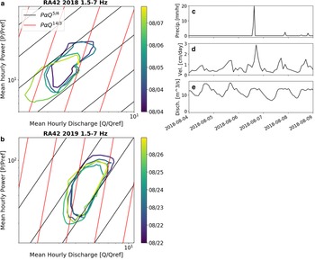
Fig. 6. Examples of the diurnal power–discharge relations observed on Rhonegletscher in (A) 2018 and (B) 2019, using data from station RA42, to demonstrate power–discharge relations during daily hydraulic activity and precipitation events. The graph explanation is the same as in Figure 5. Peak discharge measured downstream lags peak power by an hour, so the discharge values were shifted backward in time by an hour before plotting. (C) Precipitation, (D) surface velocity and (E) discharge during the 2018 example of diurnal cycling pictured in (A). Velocity measurements during the melt season were not collected in 2019. There was minimal precipitation during the time frame shown for 2019 data.

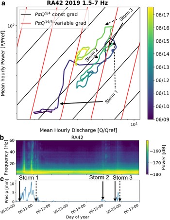
Fig. 7. The 10th and 15th June storms as observed in the (A) power–discharge relation, (B) median spectra and (C) precipitation. The graph explanation is the same as in Figure 5. Peak discharge measured downstream lags peak power by an hour, so the discharge values were shifted backward in time by an hour before plotting. Solid arrows mark the start of a storm and dotted the end of a storm. Storm 2 was small and so no specific start and end is noted, for simplicity.
Very early and very late in the melt season, the hourly power versus discharge relation is consistent with the 14/3 power of discharge expected from a variable pressure gradient ((2); Fig. 5). During the main part of the melt season, the relation follows the expected behavior of power depending on the 5/4 power of discharge, consistent with a constant pressure gradient ((3); Fig. 5). This shift between the very early/very late and mid-season behavior was also observed on Glacier d'Argentiere (Nanni and others, Reference Nanni2020) and Glacier de la Plaine Morte (Lindner and others, Reference Lindner, Walter, Laske and Gimbert2020). These full-season hourly data show a general counterclockwise hysteresis on the power versus discharge diagram, clearly in 2018 and more subtly in 2019 (Fig. 5); this hysteresis is easier to see in the daily-average data from May to September. A given discharge generates less seismic power in the early melt season (June–July) than observed in the late melt season (August–September). Again, similar behavior was observed on Glacier d'Argentière (Nanni and others, Reference Nanni2020) and Glacier de la Plaine Morte (Lindner and others, Reference Lindner, Walter, Laske and Gimbert2020).
3.3 Anthropogenic and weather impacts
Throughout the entire seismic record, there are cyclic noise bursts occurring in our range of interest (1–10 Hz) on weekdays generally between 600 and 1800 h. This appears similar to signals described by Canassy and others (Reference Canassy, Röösli and Walter2016) on Rhonegletscher, attributed to activity from nearby hydro-powerplants during the work week. The hydroelectric activity occurs throughout the winter and summer seasons. The signals we interpret as GHT do not display this weekday/weekend pattern nor occur during the winter season, so we believe these anthropogenic signals do not interfere with the GHT observations.
Disturbances to daily power–discharge relationships were often triggered by additional changes in discharge, driven by events such as a precipitation event or above/below average melt day (e.g. Fig. 6A). The compound effect of these fluctuations may contribute to the gradual progression through the seasonal counterclockwise hysteresis loop. Larger storms often include lightning, which causes short, impulsive events in the power record from induction in the cables between digitizer and seismometer, and generate thunder that is observed as oscillatory events in the seismic record (1 to 60+ Hz; Fig. 7B). While these storms caused an increase in median power, our study focuses on tremor bands that are active over a period of several consecutive days, so we are confident that storm-associated power changes do not impact our overall findings.
4. Discussion
4.1 Tremor and the channel
The GHT bands that we identify appeared immediately with the springtime increase in median power associated with discharge rising above 5 m3 s–1. These bands then persisted through the bulk of the melt season past the time of peak melt, and even in some cases after discharge values consistently remained below 5 m3 s–1. The abrupt onset of GHT may reflect the old subglacial channels swiftly creeping or melting open in response to large increases in meltwater input by spring precipitation and surface melt, while the long persistence may reflect the continued use of a well-formed channel system while it creeps closed as meltwater inputs gradually decrease. The short-duration, small swings in the generally consistent back azimuth angle for some bands during low discharge in the second half of the melt seasons and sometimes very early in the melt seasons may occur as a decrease in GHT from the main channel allows another source generating unrelated tremor at the same frequency band to dominate over the now-diminished GHT source. It is unlikely these swings are due to an actual change in channel location on the order of a few days, since the location is otherwise so consistent.
The terminal lake, which may contribute some noise to the study area, froze by 28 October 2018, and 2 November 2019, only a few days before the end of the observed GHT and melt seasons in each year. Surface wave noise from the lake should be relatively constant when unfrozen. The GHT bands are linked with occurrences of higher median power (Figs 2, 3A, C, E). The median power displays sporadic rather than continuous behavior at the end of the melt season, following changes in daily air temperatures and discharge values. The coincident time between the end of the melt season high median power and the freezing of the lake is most likely a result of both phenomena being controlled by air temperature rather than the lake being a dominant contributor to the high median power values.
The identified section of sub/englacial channel (section 1.2) is located within the back azimuth angles for almost all the GHT frequency bands at all times during both 2018 and 2019 (Fig. 4), suggesting the channel location is similar across years. This agrees with the repeated 2D surveys across several months in 2018 and 2019 (Church and others, Reference Church, Grab, Schmelzbach, Bauder and Maurer2020) and the 3D survey in 2020 (Church and others, Reference Church, Bauder, Grab and Maurer2021), which show the channel forming in the same position every year, and show a winter expression of the channel bed (perhaps sediment left in the channel) in the same position between 2018 and 2019. Since the channel forms in a similar location and reaches a similar equilibrium geometry each year (supported by our findings and by Church and others (Reference Church, Grab, Schmelzbach, Bauder and Maurer2020, Reference Church, Bauder, Grab and Maurer2021)), this has implications for processes within the ice. Using their winter GPR reflectivity, Church and others (Reference Church, Grab, Schmelzbach, Bauder and Maurer2020) speculated that the channel likely remains open and water-filled at a thickness <10 cm, or else closes essentially completely but with the sediments within the channel maintaining a permeable pathway along which the channel reforms each year. Our winter back azimuth calculations were unable to identify coherent point sources in the frequencies from 1.5 to 7 Hz, so we cannot further speculate on this possibility.
The GHT we identified on Rhonegletscher in 2018 and 2019 is dominated by Rayleigh waves in the range of 1.5–7 Hz. Upon inspecting the median seismic power between 1 and 80 Hz, the majority of seismic power measured at our stations during the study period is continuous, and between 1.5 and 10 Hz, indicating the hydraulic tremor discussed here derives primarily from turbulent water flow within and beneath the glacier, and not from processes such as sediment transport (10–20 Hz; Gimbert and others, Reference Gimbert, Tsai and Lamb2014, Reference Gimbert, Fuller, Lamb, Tsai and Johnson2019) or sliding tremor (10–90 Hz; Winberry and others, Reference Winberry, Anandakrishnan, Wiens and Alley2013; Lipovsky and Dunham, Reference Lipovsky and Dunham2016), though this does not discount that such processes are also occurring.
There are measurements of the surface ice-flow velocity from on-ice differential GPS stations near our study in the 2018 melt season, with some measurements during the early winter season in 2017 and late winter season in 2019. The velocities display distinct contrast between a summer regime (~11 cm d−1) and a winter regime (~8 cm d−1), the difference attributed to the effects of enhanced summer basal sliding (Gräff and Walter, Reference Gräff and Walter2021). Since these are similar velocity and power patterns as described by Canassy and others (Reference Canassy, Röösli and Walter2016), some of the seismic energy from 1.5 to 10 Hz may be from increased englacial fracture driven by the summer velocity regime, with the majority of the seismic power from GHT, in agreement with Canassy and others (Reference Canassy, Röösli and Walter2016). Increased summer hydrofracturing activity on Rhonegletscher is supported by Church and others (Reference Church2019, Reference Church, Grab, Schmelzbach, Bauder and Maurer2020, Reference Church, Bauder, Grab and Maurer2021), who speculated that hydrofracturing serves as the primary mechanism by which the channel forms. Church and others (Reference Church2019) also witnessed a connection between a previously unconnected borehole and the channel, which they speculated was due to hydrofracturing.
Church and others (Reference Church2019) observed the presence of immobile gravels within the englacial channel during July of 2018, supporting the hypothesis that some coarse-grained sediment is transported at some times within the channel, although transport was not occurring at the time of observation. However, in our study, we do not know when these coarse sediments are mobile and immobile. Gimbert and others (Reference Gimbert, Tsai, Amundson, Bartholomaus and Walter2016) assumed that seismic power in the range of 1–10 Hz scales with shear velocity, and related it to transported grain diameter, sediment transport flux and seismic power in the range of 10–20 Hz. However, we cannot precisely constrain the ratio of the discharge measured in Gletsch (section 2.3) that passed through the englacial channel as opposed to other pathways (described in section 4.2). We can only measure the total amount of meltwater coming from the glacier and make inferences about how much water was moving through the sub/englacial channel at the time, and so the relation between power in the 1–10 Hz range and shear velocity cannot be used to precisely infer when coarse grains were mobilized in the channel. Studies monitoring bed load transport during river floods and in laboratory flumes are better constrained (e.g. Hsu and others, Reference Hsu, Finnegan and Brodsky2011; Burtin and others, Reference Burtin2011; Schmandt and others, Reference Schmandt, Aster, Scherler, Tsai and Karlstrom2013; Gimbert and others, Reference Gimbert, Fuller, Lamb, Tsai and Johnson2019) and their methods cannot be applied here. Thus, we omit discussion of frequencies above 10 Hz with respect to sediment transport; careful consideration in future work paired with monitoring of water pressure and sediment transport within the channel might reveal interpretable signals.
4.2 Power versus discharge relations
One hypothesis for the hysteresis observed in our power–discharge relationship is that seasonal changes in water routing occur, with the GHT-generating channel capturing an increasing fraction of the discharge as the melt season progresses. The discharge measurements are collected downstream of Gletsch, as noted above, and thus capture the total meltwater running off the glacier and not exclusively water that generated GHT via turbulent flow when passing through the englacial or subglacial channels (inflow to the stream is almost entirely from the glacier). During the early melt season, the channel system is still developing, with some water flowing through a distributed system (e.g. Church and others, Reference Church, Grab, Schmelzbach, Bauder and Maurer2020). It is possible that a substantial quantity of the downstream discharge derives from water that travels through the glacial hydraulic system during the early melt season ‘quietly’ (little turbulence) via the distributed system. Later in the season when the channelized system is well-developed and better connected to basal and englacial water reservoirs (e.g. Church and others, Reference Church, Grab, Schmelzbach, Bauder and Maurer2020), the downstream discharge may contain more water that generated GHT via turbulent flow as it passed through the channel system. Thus, the seasonal counterclockwise hysteresis could arise from changing connectivity within the glacial hydraulic system. This may also relate to the changes in the GHT frequency bands noted in the results (section 3.1), which occur around the end of August/early September.
During July and August, variations in the power–discharge relation are dominated by diurnal hysteresis loops, which are similar from day to day (e.g. Fig. 6); similar features were observed in prior work on Glacier d'Argentière (Nanni and others, Reference Nanni2020). On a typical day, a few hours of the rising limb, and also of the falling limb, track close to the 5/4 power trend consistent with a constant pressure gradient (3). Shorter periods at the start and end of the day fall closer to the 14/3 power trend expected from a variable pressure gradient (2). There also are times of rising discharge with near-constant or falling noise in the evening, and falling discharge with rising noise in the early morning. These transitional periods do not scale with the constant or variable pressure gradient relations, and likely arise from complex interactions between the rate at which channels open or close in response to changing water pressure and melt rates, and the rate of change in water discharge and pressure gradient. To explain this behavior, future studies might focus on collecting high-resolution measurements of diurnal changes in velocity and pressure of water within the channel.
These diurnal patterns could reflect cycles of slow creep-closure overnight and melt-expansion during the day. The initial increase in meltwater in the morning may overwhelm the constricted night configuration for a few hours, causing the switch to a variable pressure gradient system. Once meltwater has expanded the channel to the daytime configuration, it may switch back to a constant pressure gradient system. After peak daily melt and the onset of the falling limb in discharge, the system may rapidly switch to a variable pressure gradient for a few hours while the channel experiences creep-closure to a night configuration. The plausibility of this hypothesis is explored below.
Church and others (Reference Church, Grab, Schmelzbach, Bauder and Maurer2020) conducted an in-depth analysis of the thickness of the channel from their repeat GPR surveys, and found it generally remains in the range of 0.2–0.4 m thickness across the melt season. It is possible that we have captured the signal of diurnal variations in channel height on the order of a few cm, below the resolution of the measurements in Church and others (Reference Church, Grab, Schmelzbach, Bauder and Maurer2020). Given that the channel is generally much wider than it is tall (Church and others, Reference Church2019, Reference Church, Grab, Schmelzbach, Bauder and Maurer2020, Reference Church, Bauder, Grab and Maurer2021), creep could thin it by a few cm during low discharge every night (e.g. Perol and others, Reference Perol, Rice, Platt and Suckale2015), notably decreasing the discharge capacity, resulting in a large increase in tremor during the morning melt onset in response to increasing pressure gradient along flow. An associated increase in pressure could then increase the channel height a few cm over the span of a few hours. Interactions among ongoing changes in discharge and channel size, with creep and melting rate changing, then may link the rising and falling limbs of the hysteresis cycle. This is a possible mechanism that could generate the observed diurnal power–discharge hysteresis. Similar observations were made by Nanni and others (Reference Nanni2020) on Glacier d'Argentière during early season (June) in 2017, who proposed a similar explanation.
In June, when the melt season tremor had only recently begun and the channel was not yet well-developed (Church and others, Reference Church, Grab, Schmelzbach, Bauder and Maurer2020, Reference Church, Bauder, Grab and Maurer2021), two large storms (10 and 15 June ) caused major shifts in the power–discharge relation (Fig. 7). The rapid rise in discharge during each of these storms caused a rise in power closely following the 14/3 dependence on discharge expected for a variable pressure gradient system (2), possibly because the channel geometry could not respond rapidly enough to accommodate the rapid increase in discharge. After the 15th June storm, the discharge–power values returned to constant gradient behavior, but despite returning to pre-storm discharge levels, the power was much higher. This could be explained by an increase in connectivity between the channel and englacial and subglacial water reservoirs, allowing more water, previously traveling ‘quietly’ through the distributed system, to travel via turbulent channel flow to the terminus (Fig. 7). This could have been achieved by englacial fracturing or basal lift off driven by over-pressurization when the hydraulic system was overwhelmed by rainwater, or just by rapid expansion of the channel and connections, or some combination of these. Storms later in the season were not as effective at reaching this variable pressure gradient behavior, possibly because the later-season drainage system had greater transport capacity and connectivity as a well-developed system (supported by observations in Church and others, Reference Church, Grab, Schmelzbach, Bauder and Maurer2020, Reference Church, Bauder, Grab and Maurer2021).
4.3 Wave types of GHT observed on Rhonegletscher
Vore and others (Reference Vore, Bartholomaus, Winberry, Walter and Amundson2019) proposed that the wave types identified on Taku Glacier were controlled by proximity to the source, with body waves dominating measurements made near (<1 wavelength) a GHT source and Rayleigh waves dominating measurements made farther (>1 wavelength) from a GHT source, owing to the distance required for interference of body waves to generate the surface Rayleigh waves. Assuming P-wave (v p~3800 m s−1), S-wave (v s~1800 m s−1) and Rayleigh-wave velocities (v r~1650 km s−1) in ice (e.g. Kohnen, Reference Kohnen1974) results in wavelengths of 1.9–0.54 km for P-waves, 0.9–0.25 km for S-waves and 0.82–0.23 km for Rayleigh waves in our frequency range (2–7 Hz). These estimated wavelengths place all our stations in the ‘near-field’ zone of the mapped subglacial channel. We inspected the percentage of wave types present at all stations in each year and found, in all cases, a large increase in Rayleigh waves generated with the onset of the melt season (Supplementary Fig. S2). The quantity of body and mixed wave types produced on Rhonegletscher does not appear to vary across the year, and their summer decrease in percentage of the total wave field is due to the large increase in percentage of Rayleigh waves. This clear uptick in the generation of Rayleigh waves across Rhonegletscher during the melt season appears to be responsible for the detection of only Rayleigh wave GHT. This suggests that the percentages of wave types present in GHT may derive from specific factors in the glacial system and the surrounding environment, and not purely from proximity to a subglacial and englacial channel.
Vore and others (Reference Vore, Bartholomaus, Winberry, Walter and Amundson2019) suggested that the presence of a near-field source external to the glacier (in their case, a river) likely contributed to the presence of body waves on Taku Glacier. Our stations are 0.8–1.5 km from the terminal lake and the waterfall draining into the Rhone Valley. If the waterfall were a substantial source of body waves, there would be a clear increase in the amount of body waves in the summer as the waterfall discharge increases with the melt season, which we do not witness. Additionally, we did not find any back azimuth angles that point toward the waterfall from any of the seismic stations.
5. Conclusion and future work
We conducted an analysis for GHT on Rhonegletscher in 2018 and 2019, and used FDPA to determine the wave types and polarization of the tremor and to calculate back azimuth angles to the source where possible. We applied the methods of Vore and others (Reference Vore, Bartholomaus, Winberry, Walter and Amundson2019), slightly modified to fit our setting, to two years of data. We identified power thresholds determined on a monthly basis, and analyzed all bands exceeding those power thresholds. We found bands of predominantly Rayleigh wave tremor. The same frequency bands and back azimuth angles were found in both years. The back azimuths include the known location of a major channel, which was identified in radar studies in 2017, 2018, 2019 and 2020, and accessed by borehole in 2020. Our findings suggest that the glacial hydraulic system develops and remains in the same location each year, with similar geometry, which agrees with prior studies. We also witnessed diurnal cycling in the relation between discharge and GHT, likely arising from interactions among variations in channel geometry and water discharge, pressure and pressure gradient driven by variations in daily melt. Furthermore, the seasonal variation in the discharge–GHT relation suggests possible rearrangements of the subglacial hydraulic system, with more of the water flow occurring in a distributed system earlier in the year.
Interpretation of our passive seismic data benefits from results of detailed on-ice surveys using radar, boreholes, GPS, campaign passive seismics (Nanni and others, Reference Nanni, Gimbert, Roux and Lecointre2021) and other techniques. Passive seismic monitoring is much easier to conduct than such surveys, though, and almost unique in the ease of maintaining long, continuous records. The agreement between the location and behavior of the channel determined by our passive seismic monitoring and by the geophysical surveys demonstrates the utility of passive seismic monitoring from a small network of ice-proximal bedrock-based stations as a viable, cost- and time- effective part of a comprehensive study of glacial hydrology.
Future studies could collect high-resolution measurements of diurnal changes in water current and pressure within the channel, and deploy a borehole seismometer in the ice near the channel. The resulting improved constraint on the timing and magnitude of channel discharge compared with the median seismic power from 1 to 20 Hz may allow the estimation of shear velocity according to Gimbert and others (Reference Gimbert, Tsai, Amundson, Bartholomaus and Walter2016) to estimate when coarse grains within the channel are mobilized. This also may allow for improved understanding of seismic signals generated by sediment transport within subglacial channels, and observing the change in discharge in the channel on an hourly scale will improve understanding of the observed daily hysteresis loops and flood event behavior in the power–discharge relations.
As briefly mentioned in section 3.1, the power threshold is surpassed in many continuous frequency bands in the winter that did not meet the requirements for peaks in polarization and wave type defined in our methods (Supplementary Materials S1). While the back azimuth angles calculated for 1.5–7 Hz during the winter do not suggest a coherent localized source, if these bands are related to the quiescent winter hydraulic system the above proposed borehole seismometer, left out overwinter near the summer channel location, could help elucidate this case.
Supplementary material
The supplementary material for this article can be found at https://doi.org/10.1017/jog.2022.69
Acknowledgements
This work was conducted in concert with colleagues at the Swiss Federal Institute of Technology (ETH Zürich). The fieldwork was funded by ETH Grant ETH-06 16-2 and the Swiss National Science Foundation (Grant PP00P2_183719). We thank all my colleagues at ETH Zürich who planned and executed the 2018 field campaign on Rhonegletscher to observe the channel, drill boreholes, maintain and expand the seismic network, and collect a large suite of measurements.


 Open access