


Introduction
The ice fields and ice caps of the Canadian Arctic Archipelago have been identified as being particularly vulnerable to the effects of changing climatic conditions, with dramatically increased melt rates having been observed in the past few years (Reference GardnerGardner and others, 2011, Reference Gardner, Moholdt, Arendt and Wouters2012; Reference FisherFisher and others, 2012). It is therefore important that ways are found to quantify these changes and their likely effect on future climate projections and sea-level estimates. Oblique or ground-based photogrammetry is a technique that has considerable potential to provide improved estimates of glacial runoff and flow dynamics.
Measurement of glacial change by ground-based photogrammetry has often used repeat photography separated by time intervals of several months or years (e.g. Reference Kaufmann and LadstädterKaufmann and Ladstädter, 2004; Reference Ladstaedter and KaufmannLadstaedter and Kaufmann, 2004; Reference Pitkänen and KajuuttiPitkänen and Kajuutti, 2004). Changes measured therefore tend to be significantly larger than the errors associated with individual measurements. The study described here uses time-lapse photography to determine daily changes in the surface elevation and horizontal position of a number of targets located on a slow-moving Arctic glacier (estimated annual speed of the terminus region <5 m a–1). The slow speed of glacier motion, and the short temporal interval between photos mean that the magnitude of any positional change is generally less than the potential error associated with an individual measurement. However, this is compensated for by the fact that daily observations are made on the glacier surface also means that measurements can be made through the winter, when through the year, allowing seasonal and annual patterns of surface change and motion to be determined and visualized in a way that has not hitherto been possible. The use of permanent targets the glacier surface is normally obscured by snow.
Oblique photogrammetry has been used to map glacier surface change in a number of studies (e.g. Reference Brecher and ThompsonBrecher and Thompson, 1993; Reference Kaufmann and LadstädterKaufmann and Ladstädter, 2004; Reference Ladstaedter and KaufmannLadstaedter and Kaufmann, 2004; Reference Pitkänen and KajuuttiPitkänen and Kajuutti, 2004; Reference Sanjosé and LermaSanjosé and Lerma, 2004). These surveys all used the intersected position of prominent points on the glacier surface to measure change. However, in each case the time interval between photos was irregular, with measurements only being acquired during the summer, meaning that seasonal patterns could not be derived. More regularly spaced photography was used by Reference Triglav, Fras and GvozdanovicõTriglav and others (2000), who were able to make use of a historical archive of monthly photography to measure change on Triglav glacier, Slovenia. However, in that case the photography was obtained from a low-resolution panoramic camera, so only major changes to the glacier could be documented.
In recent years, the development of structure from motion photogrammetry has made it possible to undertake mapping of glaciers and glacial landforms from ground-based photography without requiring the rigorous geometric constraints imposed by traditional photogrammetry (e.g. Reference Westoby, Brasington, Glasser, Hambrey and ReynoldsWestoby and others, 2012; Reference Fonstad, Dietrich, Courville, Jensen and CarbonneauFonstad and others, 2013). Although this technique has considerable potential for many applications, the simple geometric arrangement of cameras and targets in the current study lent itself to a more traditional photogrammetric approach.
The use of high-frequency time-lapse photography allows detailed measurements of change to be made. Reference Aschenwald, Leichter, Tasser and TappeinerAschenwald and others (2001) used daily time-lapse photography from a single 35 mm camera to investigate snow cover for the Passeier valley in the Italian Tyrol. The availability of frequent imagery may also make it possible to measure glacial surface motion. Reference Harrison, Echelmeyer, Cosgrove and RaymondHarrison and others (1992) used photogrammetric analysis to measure a surge of West Fork Glacier, Alaska, USA. Reference FallourdFallourd and others (2010) estimated relative surface velocities on Glacier d’Argentière, French Alps. Both of these studies used single cameras, where the distances to the observed points were unknown, so estimates of speed could only be inferred from other objects on the glacier surface.
High-frequency time-lapse imagery has also been used to map velocities for fast-moving Greenland outlet glaciers. Reference Maas, Schwalbe, Dietrich, Bissler and EwertMaas and others (2008) used a terrestrial laser scanner to overcome the problem of distance estimation, and combined these measurements with high-resolution terrestrial photography to estimate velocity fields close to the terminus of three Greenland outlet glaciers. Reference Ahn and BoxAhn and Box (2010) and Ahn and Howat (2010) describe the use of single camera time-lapse photography for determining velocities for a number of Greenland outlet glaciers, with the elevation differences between the camera and the glacier surface being used to estimate the distance to each point of interest. In the current study this process is reversed, with the distance between the camera and the target assumed to be known, and this distance being used to estimate the daily change in surface elevation.
Study Area
The study focuses on Fountain Glacier, which is a small Arctic glacier situated on southern Bylot Island in Canada’s Nunavut Territory. Fountain Glacier is officially designated as B26 by the Glacier Atlas of Canada (Inland Waters Branch, 1969). The terminus of the glacier is located at 72°57’45” N, 78°24’15” W (Fig. 1).
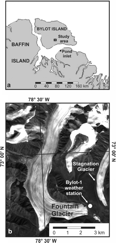
Fig. 1. Location of the study area: (a) general location; (b) Landsat 7 image of Fountain Glacier study area, supplied by Geobase®, image date 9 August 2001.
Fountain Glacier is ~ 16 km long, with the lower half of the glacier being ~ 1.2 km wide. A number of previous studies have suggested that it is polythermal in nature. Prior to the mid-1990s, its extents had changed little since the neoglacial maximum, which occurred ~ 120 years ago (Reference Dowdeswell, Dowdeswell and CawkwellDowdeswell and others, 2007; Reference Wainstein, Moorman, Whitehead, Kane and HinkelWainstein and others, 2008). However, Wainstein and others (2008) noted that significant retreat of the terminus had occurred between 1995 and 1998. They also noted that the glacier surface close to the terminus had shown average thinning rates of ~ 1 m a–1 over the 25 year period from 1982 to 2007.
The terminus of Fountain Glacier has seen major changes over the past two decades. In the early and mid-1990s it was possible to walk straight onto the front of the glacier, as it terminated in a slope. Starting in the early 1980s and continuing though the 1990s, two collapse features developed on the southern and northern sides of the terminus (Wainstein and others, 2010). Over time these two features have developed into two calving fronts, and the glacier now terminates in a 20–30 m high cliff face. In addition to surface melting, mass loss also occurs through dry calving from the northern and southern calving faces (Reference Wainstein, Moorman and WhiteheadWainstein and others, 2010).
Photogrammetric Theory
The exterior orientation parameters (EOP) of a photo are defined by three possible translations in X, Y and Z, and by the three rotation elements ω, ϕ and κ, which describe rotations around the three respective camera axes. If these six parameters are known then the position and orientation of a photo in space can be uniquely defined, as long as the inner orientation parameters (IOP) of the camera have been established. The IOP define the relationship between the camera image plane and the camera lens, and are normally derived through a camera calibration.
The principle of collinearity states that a point on a photo, the perspective centre of the camera lens and the equivalent point in the real world are linked by a straight line in space. The relationship between these elements can be expressed mathematically through the collinearity equations (Reference Wolf and DeWittWolf and DeWitt, 2000), with each ground control point (GCP) allowing the formation of two such equations. Thus three GCPs will permit the formation of six equations, which is sufficient to solve for all six unknowns. The determination of orientation parameters in this manner is known as a single-photo resection (SPR) (Reference Wolf and DeWittWolf and DeWitt, 2000). In practice the solution is normally overdetermined, with optimal values for each parameter being calculated through a least-squares adjustment. If the camera position is already known through independent measurement, then only the rotation elements need to be determined, for which a minimum of two GCPs are required.
When a stereo pair of photos is used for measurement purposes, the EOP for both photos are normally established simultaneously through an exterior orientation (EO) process. Common points on the two images are first used to create a relatively oriented model. A seven-parameter Helmert transformation is then used to fit the model coordinates to the real-world coordinate system, by applying three shifts, three rotations and a scale factor to the model. A Helmert transformation requires the X, Y and Z positions of at least three well-distributed GCPs to be known. Additional horizontal and vertical GCPs and tie points are usually added in order to improve the accuracy of this procedure, with the final orientation parameters being derived through a rigorous least-squares adjustment, which determines the optimal solution by minimizing the errors in the input data. If the positions of the cameras are already known, these can be used to constrain the adjustment. Where the EOP of each photo have already been determined independently, these parameters can be used to directly form the oriented three-dimensional (3-D) model. While not as rigorous as carrying out a full EO, this process can allow the formation of a 3-D model in circumstances where there would otherwise be insufficient control, or when GCPs and tie points common to both images cannot easily be identified.
Once a model has been oriented, measurements can be made of 3-D point positions. Point positions are calculated by the intersection of theoretical rays which are projected from the measured point on each photo, through the perspective centre of the respective camera lenses and into object space.
Methodology
Fieldwork
In August 2008, two camera stations were established high on the valley sides, overlooking the northern terminus region of Fountain Glacier. Camera stations consisted of identical 10 Mp Canon XTi cameras, with 50 mm lenses. The cameras were secured inside weatherproof enclosures, designed by Colorado (USA)-based company Harbortronics. The complete assembly comprised a solar panel, battery, backup battery and a time-lapse controller. The cameras were set up in a highly convergent configuration (Fig. 2a), which allowed for a greatly extended baseline between the two cameras, making it possible to obtain strong intersection angles at all the targets.
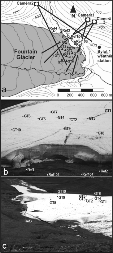
Fig. 2. (a) Camera stations and target positions during all 3 years of the study; (b) view from camera station 1; (c) view from camera station 2. The view from camera station 3 is similar to the view from camera station 1.
Four 0.6 m diameter reference targets were attached to large stable rocks located in front of the glacier, such that two reference targets were visible from each camera. These were located at a distance of ~ 500 m from the respective camera station. Ten targets, GT1–GT10, were also set up on the glacier surface. The targets consisted of 0.6 m diameter red circles against a white plastic backdrop, and were designed to be clearly visible on the camera images. Measurements of glacial surface change are normally carried out using ablation stakes, which are drilled into the ice surface. However, to measure changing surface elevations photogrammetrically it was necessary for the targets to be located directly on the glacier surface. The glacier targets were mounted on metal tripod stands for stability, with the target centres being ~ 0.5 m above the ice surface. Targets were oriented to ensure optimal visibility from both cameras. The positions of the camera stations and all targets were surveyed using a Trimble real-time kinematic (RTK) GPS system, with an estimated horizontal and vertical accuracy of 5 cm. The locations of all camera stations, reference targets and glacier targets are illustrated in Figure 2a. Figure 2b and c show photos taken from camera stations 1 and 2 respectively.
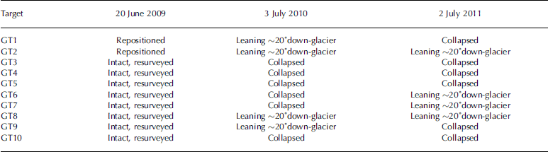
Targets were surveyed and replaced as required during follow-up visits in June/July 2009, June/July 2010 and June/July 2011. In 2009 all targets were found to be intact. However the initial measurement period did not include an ablation season, so there was little surface melting to affect target stability. In 2010 and 2011 many of the targets were found to have collapsed, as high amounts of lean caused the tripod stands to become unstable and topple over. Surviving targets in both years consistently showed leans of ~ 20° in the down-glacier direction, equivalent to the observed target centres being ~ 0.17 m further down-glacier and 0.03 m lower than they would have been had the target remained upright. The condition of each target as found in each year is listed in Table 1. All target positions were surveyed both as found, and after they had been re-established, using the Trimble RTK GPS system.
Table 1. Condition of targets as found during each field visit
In June 2010, camera 2 was moved to a new position, camera station 3, which was 84 m from camera station 1 (Fig. 2a), and the two cameras were arranged to provide stereo coverage of the northern terminus region. The two reference targets which had been visible from camera station 2 (Ref3 and Ref4) were also moved, so that all four reference targets were visible from both camera station 1 and camera station 3. These targets were named Ref103 and Ref104 (Fig. 2b).
Data retrieved
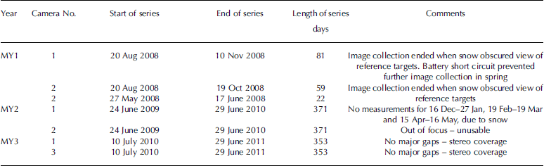
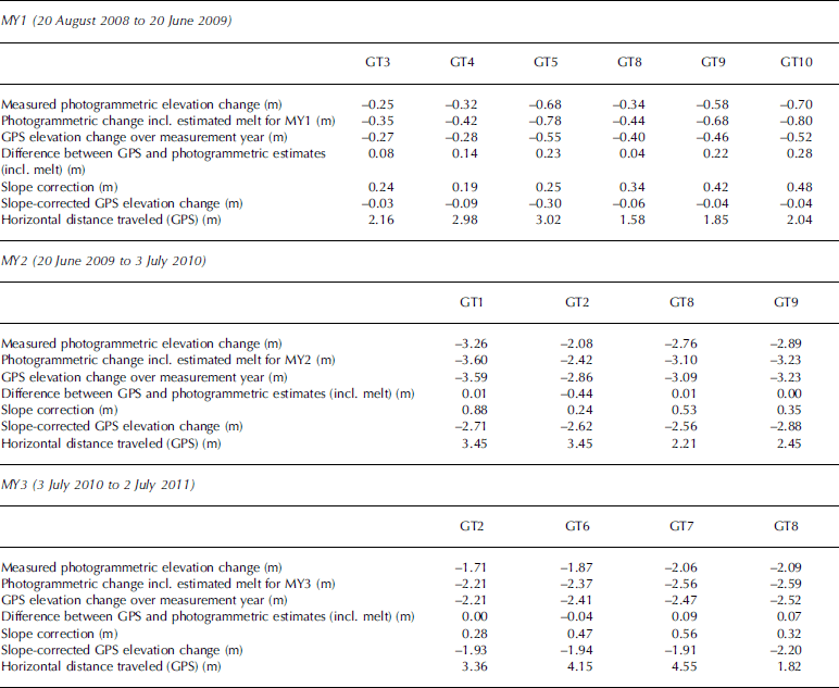
The study was divided into three measurement years (MYs), which were defined according to the dates of GPS data collection. MY1 covered the period 20 August 2008 to 20 June 2009, MY2 ran from 20 June 2009 to 3 July 2010, with MY3 covering the period 3 July 2010 to 2 July 2011.
Table 2 lists the photographic data record retrieved from each camera over the 3 years of the study. In MY2 and MY3 it was possible to retrieve images through the winter period, although blowing snow over the winter of 2009/10 resulted in three major gaps in the data series. Images from camera 2 were also found to be out of focus during MY2 and so could not be used for further analysis. However, in general the quality of the photography was found to be sufficiently good to allow target identification and analysis. The use of variable exposure times meant that targets could be clearly identified even on photos taken in the middle of winter, when Arctic latitudes experience 24 hours of darkness.
Table 2. Photographic data series collected during each measurement year
Data processing
A very simple inner orientation was assumed, with the only variable parameter being the camera focal length. In all cases the principal point was assumed to be located in the centre of the camera image plane, and lens distortion was assumed to be negligible. These assumptions could be made because it was the relative motion of the targets that was of interest, and because the target positions changed by only a few metres over the course of a year, as listed in Table 3. The camera positions were considered to be fixed throughout the study, with the ω, ϕ and κ rotation parameters for each photograph being derived from observations to the permanently installed reference targets. The separation of these targets was also used to determine the scale factor for each photograph, relative to that of the first photo in the series. The process of obtaining camera EOP was thus considerably simplified, since only the ω, ϕ and κ rotations and the focal length were required for each photo. Also because only the relative focal length was required, its initial value needed only to be determined approximately.
Table 3. Elevation change and horizontal distance traveled at each target for each measurement year
In order to derive the ω, ϕ and κ rotation parameters for each photo, measurements were made of photo coordinates for the visible reference targets and for each glacier target. The assumption was made that camera and reference target positions remained fixed throughout, which was verified through repeat GPS measurements made in 2010 and 2011. A single photo resection was carried out from each camera station after it had been set up, to obtain preliminary estimates for the focal length and the ω, ϕ and κ rotation parameters for each camera. For each photo, the separation between the reference targets was measured and this value was used as a scale factor to adjust the focal length, relative to the initial value. Sequential adjustments were then applied iteratively to the values of ω, ϕ and κ, until the calculated photo coordinates of the reference targets matched the actual measured coordinates. The process of deriving the rotation elements is described in detail by Reference WhiteheadWhitehead (2013).
For MY1, a series of daily oriented photogrammetric models was produced for the initial 59 day period, during which photos were available from both cameras. Because the camera configuration was highly convergent and because only two reference points were available for each photo, models were formed by using the EOP calculated for the individual photos, rather than using a more rigorous EO procedure. Daily X, Y and Z positions for each target were then calculated by space intersection. The positions of targets GT3, GT4, GT5, GT8, GT9 and GT10 were calculated; however, GT1, GT2 and GT6 could not be reliably identified on photos from camera 2, so were omitted from the analysis. GPS measurements made of the target positions on 20 August 2008 and on 20 June 2009 allowed estimated daily horizontal positions to be interpolated for each of these targets, with the speed of motion assumed constant. Target elevations were calculated independently using photos from camera 1 only and also using the interpolated target positions. Between 27 May and 20 June 2009, a daily series of photos was collected from camera 2 only, with target elevations being derived in the same way. Since the elevation change, rather than the absolute elevation, was of interest, derived elevations were for the centres of the targets, and were not corrected to the glacier surface.
Over MY2, target X and Y positions were interpolated from GPS observations made on 20 June 2009 and 3 July 2010. While no direct measurements were available for flow rates over the summer, the flow rates derived from GPS measurements made on 20 August 2008 and 20 June 2009 were taken to represent winter conditions. It was assumed that any accelerated velocity at the start and end of this period would likely be too small to have a significant influence on the winter average flow. This allowed estimated summer flow rates to be inferred for each target, with accelerated summer velocities being assumed for the period not covered by winter flow, i.e. 20 June to 20 August. This is a considerable simplification, since summer flow could potentially vary considerably both in speed and duration. However, typical winter velocities at most targets were of the order of 1 cm d–1, so any errors introduced by this assumption were considered to be small, and would likely have had a negligible effect on the final derived elevations. The repositioned targets GT1 and GT2 were only established in June 2009, so their displacement was estimated proportionally, with summer velocities being assumed to be 50% greater than winter velocities, a factor which approximately matched the average differences observed at the other targets. As the other targets had collapsed, a full set of elevation measurements could only be computed for GT1, GT2, GT8 and GT9. There were several gaps over the winter caused by snow obscuring the targets, with targets intermittently becoming visible for several days as the wind blew the snow clear (Table 2).
In MY3, the determination of target positions and elevations was carried out using two different methods. The first method used interpolated X and Y positions derived from GPS measurements made on 3 July 2010 and 2 July 2011, with the estimated target positions being calculated in the same way as for the previous years. Measurements were made using photos obtained from camera 1, and used to calculate weekly elevation values for each target on the glacier surface. Stereo analysis was also carried out, using Inpho photogrammetric software. A series of 3-D models was created, using photos from cameras 1 and 3. Reference targets Ref1, Ref2 and Ref104 were used as GCPs, with the glacier targets being used as tie points. The camera positions were held fixed, and their focal lengths were adjusted according to separate scale factors derived for each camera, using the separation of the reference targets. Coordinates were calculated weekly through the summer of 2010, and daily between 15 and 29 June 2011. It was only possible to track targets GT102, GT106, GT107 and GT108 through MY3, as all the other targets collapsed. A comparison between the derived surface elevations calculated using the two different methods showed no significant differences, with the 3-D coordinates derived by stereophotogrammetry providing a useful check on the accuracy of elevations derived from camera 1 alone.
Estimation of surface melt rates
To account for the difference in the measurement periods between the photogrammetric series and the GPS observations, estimated melt rates for the missing data from each year were calculated as follows:
-
For the last 3 days of MY1, estimated melt rates were calculated using the averaged regression-line slope derived from the photogrammetric elevation differences at each target over the preceding week, giving an estimated melt of 0.1 m over the 3 days.
-
For the first 4 days of MY2, estimated melt rates were calculated using the averaged regression-line slope derived from the photogrammetric elevation differences at each target for the following week, giving an average ice loss of 0.12 m over the 4 days. To determine the average melting for the last 4 days of MY2, 16 targets across the glacier terminus which formed part of a related study were used. These were surveyed on 30 June and 6 July 2010, giving an estimated melt of 0.22 m over 4 days.
-
Estimated melting for the first 7 days of MY3 was also derived from the same measurements, giving an estimated melt of 0.375 m. For the last 3 days of MY3, the ice loss was estimated using the averaged regression-line slope derived from the preceding week of photogram-metric measurements, with values at each target being averaged, giving an estimated melt of 0.12 m.
Calculating 3 year surface elevation changes
The GPS elevations for each target were accepted as definitive and were used to constrain the combined photogrammetrically derived elevation differences and estimated melting for each measurement year. Residual differences were redistributed through the photogrammetric data series. To prevent the start and end of the photogrammetric series from being skewed by atypical elevation values, the starting and ending elevations for each measurement period were determined by fitting a linear regression line to the first five and the last five daily observations for each measurement year respectively.
It was also necessary to compensate for the vertical component of down-glacier motion, which would cause the surface elevation of each target to drop over time as it moved down-glacier, even if no melting occurred. The difference in height due to surface slope was estimated for each target, using a 1 m resolution digital elevation model (DEM) produced in a 2010 survey, which was carried out using an unmanned aerial vehicle (Reference Whitehead, Moorman and HugenholtzWhitehead and others, 2013). The derived correction was then added to the calculated elevation change, in order to estimate the change in elevation that would have occurred had the target remained stationary (Table 3).
Measuring horizontal motion
Because horizontal motion is measured by intersection, changes in X, Y position could only be calculated for the first 59 days of MY1. In MY3, imagery from two cameras was available. However, the 84 m baseline was considered too short to give reliable results. For the MY1 measurements, all horizontal motion was considered to be relative to the first photogrammetric observation, made on 20 August 2008.
Results
The results for all three measurement years are listed in Table 3, with profiles for each standing target illustrated in Figure 3. Scaled and corrected elevation changes for all standing targets were averaged for each measurement year, and the 3 year average profile is illustrated in Figure 4. Figure 4 also provides information about patterns of melt and ice accumulation in each balance year (BY), defined as the period between successive annual minima in the mass of the glacier (Reference Benn and EvansBenn and Evans, 1998). Balance-year start dates were estimated from analysis of the 3 year average elevation profile (Fig. 4), and taken as being the point at which the profile reached a minimum after the summer ablation season. Using this method, BY1 was estimated to start on 9 September 2008, BY2 on 11 September 2009 and BY3 on 16 September 2010, corresponding to points A, C and E in Figure 4. Each ablation season was estimated to start where the average profile reached a maximum prior to the start of surface melting. These points occurred on 6 June 2009, 16 June 2010 and 10 June 2011, corresponding to points B, D and F in Figure 4. Table 4 shows the averaged seasonal elevation changes calculated for each balance year (after correction for down-glacier motion).
Table 4. Average change in elevation for summer and winter of each balance year
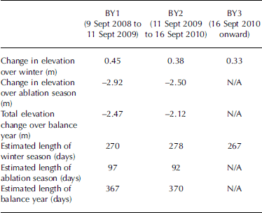
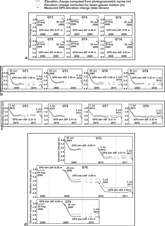
Fig. 3. Measured elevation changes for all targets: (a) MY1, (b) MY2, (c) MY3 and (d) multi-year profiles for targets standing for >1 year. Uncorrected elevation change is shown as a solid line, with profiles corrected for vertical motion indicated by a dashed line. Dates refer to the timing of the GPS measurements, which define the start and end of each measurement year.
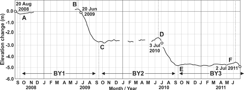
Fig. 4. Average surface elevation change derived from all standing targets measured at the end of each measurement year, after correction for down-glacier motion. A, C and E represent post-ablation-season minimum elevations for 2008, 2009 and 2010 respectively. B, D and F represent pre-ablation-season maximum elevations for 2009, 2010 and 2011 respectively. Dates refer to the timing of the GPS measurements, which define the start and end of each measurement year.
Analysis
The elevation profiles in Figures 3 and 4 reveal the distinct pattern of seasonal variations in surface elevation for the glacier terminus region. It should be noted that because the target stands rested on the underlying glacier surface, the presence or absence of snow cover did not affect the derived elevation changes. The duration of the study covered three winters and two ablation seasons. The profiles show evidence of a recovery in the ice surface of 0.3–0.5 m each winter, likely due to ice flow from higher up-glacier.
It can be seen from Table 4 that during the 2009 ablation season the glacier surface elevation dropped by an average 2.92 m, whereas over the 2010 ablation season the corresponding drop was 2.5 m, which is likely to be at least partly due to the fact that the 2009 ablation season was 5 days longer than the 2010 season. Figure 4 also shows that the surface level dropped more steeply in 2009 than in 2010, suggesting that greater temperature-related melting occurred in 2009.
It is likely that inflow of ice to the terminus region from higher up-glacier will be greatest in the summer, due to more rapid summer flow rates. The derivation of winter and summer surface flow rates was carried out using GPS measurements obtained on 20 August 2008, 20 June 2009, 3 July 2010 and 2 July 2011, with winter flow being assumed to be dominant over the period 20 August 2008 to 20 June 2009. Annual flow rates calculated from all GPS measurements are shown in Table 3. From a comparison of the GPS measurements it was inferred that summer flow rates were ~ 150% of the winter flow rates, when averaged across all targets. This is a simplification, but it is sufficient to allow an approximate estimation of the relative amount of ice inflow over the summer, compared with that over the winter period.
The winter surface rise of 0.3–0.5 m noted above for each target was averaged to give a ~ 0.4 m rise across the terminus region from winter ice inflow. Since summer flow rates were estimated to be 150% of winter flow, it was estimated that ice flow from higher up-glacier would contribute ~ 0.2 m to surface elevations during the 3 month ablation season. This suggests that the values for seasonal ablation illustrated in Figure 4 and listed in Table 4 are underestimates, and that total melt should actually be ~ 3.1 m for BY1 and ~ 2.7 m for BY2. If it is assumed that ice inflow from higher up-glacier contributed an average 0.6 m to the surface elevation, then ice loss from melting close to the terminus would likely have exceeded ice inflow by a factor of ~ 5:1 during both 2009 and 2010.
It was possible to infer the start and end of each ablation season from the elevation profiles. Point A in Figure 4 defines the minimum surface elevation reached at the end of the 2008 ablation season, which corresponds to the start of BY1. Points B, C, D, E and F define the start and end of the 2009 and 2010 ablation seasons and the start of the 2011 ablation season respectively. To see how these points corresponded with the temperature record, they were plotted against the respective daily average and minimum temperature records from the nearby Bylot-1 weather station (Fig. 1), with this comparison being illustrated in Figure 5. It can be seen that there is good agreement between the timing of the maxima and minima identified on Figure 4 and the date when the average daily minimum temperature crossed the freezing mark in both years. As such, this measure appears to be a better indicator of the start and end of the ablation season for this part of Fountain Glacier than the average daily temperature.

Fig. 5. Plot of minimum and average daily temperatures recorded at the Bylot-1 weather station for MY2 and MY3. Notice the strong correspondence of the maxima and minima illustrated in Figure 4 with the minimum daily temperature.
Comparison with Bylot-1 temperature record
For the 2009 and 2010 ablation seasons, the mean daily temperature observed at the Bylot-1 weather station was used to compute the estimated amount of surface melting. This was done by calculating the cumulative daily temperature over the ablation season, using points B and C, and D and E, identified in Figures 4 and 5 as the starting and ending days for the 2009 and 2010 seasons respectively. By empirical matching, a multiplier of –0.0043 was found to give a good fit between the cumulative temperature (°C) and the photo-grammetrically derived change in surface elevation (m). To allow direct comparison, elevation changes derived from the temperature series were matched to the photogrammetrically derived elevations on the date that GPS observations were made in each year. The comparison is illustrated in Figure 6, and it can be seen that there is strong agreement between the two datasets, except at the start and end of the two ablation seasons, when average daily temperatures approach the freezing mark. It should be noted that this empirical relationship does not account for the estimated 0.2 m of surface rise resulting from ice inflow over each ablation season. However, if the amount of surface change arising from ice inflow could be accurately determined through the ablation season, a simple modification of the coefficient could be made to compensate for this effect.

Fig. 6. Comparison between photogrammetrically derived (solid line) and temperature-derived (dashed line) elevation changes for (a) 2009 and (b) 2010.
Using empirical ice-melt profiles derived from temperature can also provide an alternative way of filling gaps in the photogrammetric series, such as the time difference between the start and end of photogrammetric observations and the timing of GPS measurements. Using this technique, the estimated melting for the last 3 days of MY1 was calculated at 0.07 m, compared with the value of 0.1 m used in the analysis. The first 4 and last 4 days of MY2 were estimated at 0.11 and 0.15 m respectively, compared with the values of 0.12 and 0.22 m used in the analysis, while estimated melt for the first 4 days of MY3 was 0.34 m, compared with the value of 0.375 m used.
Horizontal measurements
Photogrammetrically derived changes in X and Y were calculated for the first 59 days of MY1 by intersection. Results are illustrated for targets GT3, GT4, GT5, GT8, GT9 and GT10 in Figure 7. Average values for distance travelled per day, change in easting and change in northing were determined by linear regression from the photogrammetric data series. These results are summarized in Table 5. The changes in easting, and the total distance travelled down-glacier generally had high R 2 values, indicating a strongly linear trend. However the changes in northing showed much lower R 2 values, most likely because the north/south component of motion at all targets was relatively small. To estimate the accuracy associated with the calculated XY positions, the individual observations were compared to the theoretical coordinates interpolated from GPS measurements. These were calculated from GPS measurements made on 20 August 2008 and 20 June 2009 at each target, with down-glacier motion assumed to be constant. The comparison produced root-mean-square errors (RMSE) of <0.05 m for both eastings and northings at all targets, suggesting that the accuracy associated with individual observations in MY1 was relatively good. Since little speed variation was expected to occur over the winter period, it was concluded that down-glacier surface speed and direction could be predicted from the photogrammetric observations with a high level of confidence.
Table 5. Comparison of photogrammetrically and GPS-derived distance and direction of surface motion for MY1
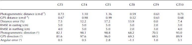
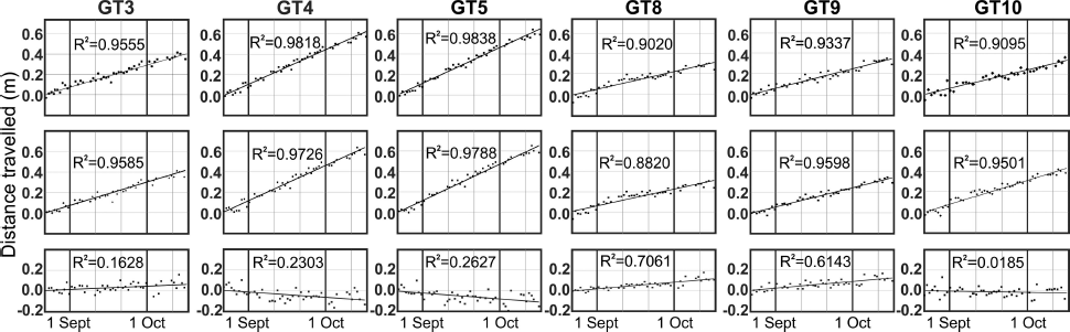
Fig. 7. Horizontal distances measured photogrammetrically during first 59 days of MY1. The top row represents the total distance travelled from the starting point, with the average speed being derived from the slope of the regression line. The middle row represents the amount of eastward travel, with the bottom row representing the amount of northward travel. The direction of travel was derived from the ratio of regression lines fitted to each of these data series.
Accuracy Assessment And Sources Of Error
In this section possible sources of error are examined, along with their potential contribution, with a view to determining estimates of the accuracy of all measurements made using ground-based photogrammetry.
Photo measurement errors
From repeated measurements of multiple targets, it was determined that the target centres could be consistently estimated to within half a pixel. Each target was 0.6 m in diameter, which at a distance of 500 m is represented by ten pixels. The centre of the reference targets could thus be identified to an accuracy of ~ 3 cm. For the targets located on the glacier surface, the accuracy was estimated at 3–7 cm, depending on distance from each camera. To test the effect of errors in the measurement of the reference targets, row and column coordinates for these targets were varied systematically in X and Y by up to three pixels, with revised positions of the targets on the glacier surface being recalculated for each permutation. These tests showed that a one-pixel measurement error for one of the reference targets could potentially introduce elevation errors of 4–8 cm, depending on the radial distance of a target from the centre of the image, and on its distance from the camera. Combining errors from both sources suggests that the maximum potential measurement error associated with each target was in the range 8–15 cm, under good conditions.
The effect of baseline length on the accuracy of intersected positions
For stereo aerial photography the relationship between image parallax and height resolution was described by Reference PetriePetrie (1970) as
where dp is the difference in parallax of the point as measured on both images, f is the focal length of the camera lens, B is the baseline distance between the two camera positions, H is the height above ground level and dh is the height difference associated with change in parallax dp. For oblique photogrammetry, depth can be substituted for flying height. It can be seen that the accuracy of a measurement therefore depends on the ratio of the photographic base length to the square of the distance to the point being measured. If it is assumed that there is a potential half-pixel error associated with each target measurement, there is therefore a potential measurement error of up to one pixel associated with each photo pair. If this measurement error is substituted for parallax then Eqn (1) can be rewritten as
where dp is the error in the photographic measurement, which is expressed in image coordinates, with one pixel being equal to 5.86 µm for the Canon XTi. D represents the depth, defined as the 3-D perpendicular distance between the baseline and the target, f is the camera focal length and B is the baseline.
The distance between camera stations 1 and 2 was 940 m, and the perpendicular distance to the targets varied between 500 and 800 m, giving a range of possible errors between 3 and 8 cm in the estimated distance to the targets, which shows reasonable agreement with the RMSE calculated for the XY position of each target over the first 59 days of MY1.
The effect of errors in XY position on elevation
Errors in the target XY position will affect the derived elevation. For interpolated coordinates this uncertainty will be systematic, reaching a maximum midway through the measurement period, whereas errors in intersected positions will be random. Because of the relatively short distances moved by the targets, and because the movement generally occurred in a consistent direction, the uncertainty in XY position was considered unlikely to have exceeded 0.5 m. The vertical errors which would result from a 0.5 m error in horizontal position were calculated for each target. They varied between 5.7 cm at GT4 to 8.8 cm at GT9. For targets fixed by intersection, based on the RMSE listed in Table 5, it was estimated that the vertical error resulting from positional uncertainty ranged between 0.5 and 1 cm.
The effect of focal length variations
Both cameras showed significant variations in focal length over the study. A scale factor was computed for each image by measuring the separation of the reference targets, and comparing it with the initial value when the camera was set up. This scale factor was then used to compute a new value for focal length (Reference WhiteheadWhitehead, 2013). The variations in focal length for cameras 1 and 3 over MY3 are illustrated in Figure 8. It can be seen that the focal lengths for both cameras changed by ~ 0.3 mm over this period, which is equivalent to a scale change of ~ 14 pixels, or ~ 0.4 m over the measured distance between the reference targets. The change in focal length at both cameras appears to be correlated, suggesting that the variation may be related to changing temperatures. Similar scale variations were also apparent for MY1 and MY2. In general, residual scale errors are expected to be small, and probably contributed no more than 10 cm at maximum to the derived target positions and elevations after corrections were applied.

Fig. 8. Variation of camera focal length over MY3.
Stability of camera stations
All three camera stations showed some rotational instability, with camera station 2 showing a change of >1° in ω during September 2008 and again in June 2009. However, the associated elevation profiles showed no sign of these variations, suggesting that rotation parameters were correctly determined. In MY2, camera 1 showed only small changes in rotation parameters. In MY3, both camera 1 and camera 3 showed only small rotation changes.
Snow cover and poor visibility
Analysis of the photos from camera 1 suggested that the lower parts of most targets were obscured by snow during the latter part of each winter. For targets half obscured by snow, this could potentially introduce a 15 cm elevation error. In such cases, the centre position was estimated from the top of the target, using the known target size from observations made in snow-free conditions. Even after adopting this strategy, it is estimated that partially obscured targets could potentially result in vertical errors of 5–10 cm.
Where visibility was poor due to atmospheric conditions, it was estimated from repeat measurements that measurement errors of up to two pixels could potentially be made, which would suggest that individual target elevations could potentially be in error by up to 15 cm. Generally such errors were isolated and it is not believed that they had a significant effect on the overall shape of the elevation profiles. Measurement errors of up to two pixels in the reference targets were also possible, especially for target Ref2, which was often difficult to see against the background in snowy or foggy conditions.
GPS errors
Targets and camera positions were surveyed using a Trimble dual-frequency GPS receiver, operating in RTK mode. Typically this would be expected to deliver relative horizontal and vertical accuracies in the 1–2 cm range. A horizontal and vertical accuracy of 5 cm was assumed, to account for the difficulty of precisely measuring the exact centres of the targets. The base station was established at the nearby Bylot-1 weather station, in the same position each year. However, there is always the possibility of incorrect GPS positions arising from poor identification of target centres, or from incorrect antenna heights being entered.
Target lean and target collapse
In 2010 and 2011, it was found that most targets had developed a significant amount of lean or had collapsed completely. Since the centres of the targets were ~ 0.5 m above the ice surface, this could potentially have introduced significant vertical and horizontal errors in a number of cases. It is estimated that a lean of 20° down-glacier would cause the position of the target centre to change by 0.17 m horizontally, and 0.03 m vertically, compared to an unaffected target. To minimize inaccuracies, targets that collapsed were omitted from the analysis. Similarly, most targets sunk into the ice surface by ~ 0.2 m over time. It was observed that most of this sinking occurred during the first few days after target placement, with targets remaining relatively stable after this time.
Overall accuracy
In a worst-case scenario, a combination of the above errors could potentially have introduced uncertainties of 0.5 m or greater into the photogrammetrically derived elevations during each year of the study. However, it is unlikely that all of these effects were present at all targets, and it is also unlikely that they would have been cumulative. It is therefore believed that the calculated profiles can be considered to be substantively correct, giving a realistic view of elevation changes on the glacier surface over the duration of the study. The averaged 3 year profile illustrated in Figure 4 is most likely to be representative of overall conditions, since the effects of any residual errors are likely to be reduced through the averaging process. To give an idea of the variability of measurements, the standard deviation (SD) was calculated for elevation measurements made over the winter of MY3, when little natural variation would be expected to have occurred. The mean SD for targets GT2, GT6, GT7 and GT8 was found to be 0.08 m, suggesting that, in general, measurements had a higher level of consistency than the above analysis suggests.
Discussion And Conclusions
The results from this study show how it is possible to measure both elevation change and horizontal and vertical motion of the glacier surface using time-lapse photography, acquired by permanently installed cameras. The application of these techniques builds on previous studies that have made use of ground-based photogrammetry (e.g. Reference Brecher and ThompsonBrecher and Thompson, 1993; Reference Kaufmann and LadstädterKaufmann and Ladstädter, 2004; Reference Pitkänen and KajuuttiPitkänen and Kajuuttib, 2004), as well as studies that have made use of time-lapse photography for the measurement of glacial processes (e.g. Reference Harrison, Echelmeyer, Cosgrove and RaymondHarrison and others, 1992; Reference Maas, Schwalbe, Dietrich, Bissler and EwertMaas and others, 2008; Reference Ahn and BoxAhn and Box, 2010; Reference Ahn and HowatAhn and Howat, 2011). However, in this case, time-lapse photography has been used to measure the comparatively small displacements associated with slow-moving Arctic glaciers, thus demonstrating the feasibility of obtaining year-round measurements of glacial surface change in Arctic environments. Because the results form a continuous series, rather than comprising multiple snapshots, the approach outlined above provides researchers with a way of viewing both seasonal and longer-term changes. Such techniques can potentially be applied to other valley glaciers, allowing improved estimates of the timing and magnitude of seasonal runoff.
Elevations calculated from interpolated coordinates using a single camera agreed closely with those calculated using intersected coordinates, which suggests that in the case of Fountain Glacier and many other slow-moving glaciers, accurate information on surface elevation change can be obtained using a single camera, along with supporting GPS measurements. It is likely that this will not be the case for faster-moving temperate glaciers, where interpolated XY positions are likely to be less accurate. In such cases, it is likely that two cameras will be necessary to calculate horizontal positions to the required level of accuracy. Many faster-moving glaciers may also not be suitable candidates for such an approach because it may prove difficult to install permanent targets on the glacier surface, and targets in high-snowfall areas are likely to be obscured during winter months.
The use of ground-based photogrammetry made it possible to measure changes in glacier surface elevation over a 3 year period. From this information it was possible to accurately track ice melt through the ablation season, and to measure the surface rise due to ice inflow over the much longer winter period. From these measurements it was estimated that ice melt for the terminus region of Fountain Glacier exceeded the inflow of ice from higher up-glacier by a factor of ~ 5: 1, over the duration of the study.
From photogrammetric measurements it was also possible to determine when the ablation season started and ended to the nearest day, making it possible to obtain reliable estimates of the start and end of the balance year. It was found that the dates when the averaged minimum daily temperature at the nearby Bylot-1 weather station crossed the freezing mark agreed closely with the dates for the start and end of the ablation season derived from photogrammetry. Ice melt estimates were also derived from the average daily temperatures at the Bylot-1 weather station over the 2009 and 2010 ablation seasons. These showed a clear correlation with photogrammetrically derived changes in surface elevation over both years, providing additional evidence that the photogrammetrically derived elevation profiles correctly reflect changes in surface elevation. Comparison of temperature-derived and photogrammetrically derived profiles may also provide a means of detecting surface elevation anomalies, such as those produced by variations in basal water pressure.
It was also found that by using regression analysis of intersected positions measured from two cameras, XY positions of targets relative to their starting positions could be calculated to an accuracy of better than 0.1 m, even at distances of 500–800 m from the cameras. Where photos were only available from a single camera, the use of interpolated coordinates, derived from annual GPS measurements, was found to be sufficiently accurate to obtain good estimates of surface elevation.
The ability to apply photogrammetric analysis techniques to digital time-lapse photography opens up new possibilities for the analysis of dynamic processes, both in glaciology and in other geomorphic environments. By using targets with positions constrained by GPS measurements, it was possible to determine motion patterns and changes in surface elevation throughout the year, including times when researchers were not present in the field. While the accuracies associated with individual measurements may be limited, the fact that daily, or even hourly, measurements can be obtained allows elevation changes and surface dynamics to be analysed in a completely new way. The use of such techniques may therefore help to shed new light on glacial processes in the Arctic and beyond.
Acknowledgements
We acknowledge the Northern Scientific Training Program and the National Science Research Council of Canada for providing funding for this project, and the Polar Continental Shelf Program and Parks Canada for providing logistical support. We also acknowledge the contributions of two anonymous reviewers, whose comments greatly improved the final paper.


