


1. INTRODUCTION
On glaciers, the annual variations of the mass-balance result in snout fluctuations with a time lag that depends on both their morphological characteristics and the meteorological forcing. The glacier length changes expressed by snout fluctuations can therefore be considered a proxy of the mass balance (Oerlemans, Reference Oerlemans1994; Hoelzle and others, Reference Hoelzle, Haeberli, Dischl and Peschke2003).
Field measurements of glacier length variations have been carried out in the European Alps since the late 19th century (Citterio and others, Reference Citterio2007; Zemp and others, Reference Zemp2015; Fischer and others, Reference Fischer2018); they are available in web archives such as the World Glacier Monitoring Service (http://wgms.ch/) (WGMS, Reference WGMS2015). The major part of the available field data refers to glaciers of large or medium size, while very small glaciers (< 0.5 km2), representing ~80% of the total number in temperate mountains (Huss and Fischer, Reference Huss and Fischer2016), are ignored for both their small size and inaccessible location, possibly introducing a bias in the quantification of the current trend and of the expected glacier changes.
In the 1980s, on the Italian side of the Alps, 1397 glaciers with a total area of 608 km2 were identified on the basis of data collected for the World Glacier Inventory (Serandrei-Barbero and Zanon, Reference Serandrei-Barbero, Zanon, Williams and Ferrigno1993); more recently, only 903 glaciers have been catalogued, 84% of them with areas < 0.5 km2 and 9.4% > 1 km2 (Smiraglia and Diolaiuti, Reference Smiraglia and Diolaiuti2015). In both glacier inventories, the areas were obtained from aerial photographs integrated with ground surveys. Despite their small size, the large fraction of small glaciers implies that they affect the Alpine landscape, its biodiversity and geodiversity, and the land use in the full basin, trasforming the nival and pluvial regime into a mixed runoff system. The possibility of their extinction due to ongoing climate change is therefore of great interest. The largest part of these glaciers belongs to the mountain type (mainly cirque, niche and slope glaciers). They differ from the valley glaciers by the absence of the valley tongue (Cogley and others, Reference Cogley2011).
According to Roe and O'Neal (Reference Roe and O'Neal2009) and Oerlemans (Reference Oerlemans2011), a first-order linear differential equation (hereafter the linear model) linking the glacier snout to air temperature fluctuations is the simplest approach to reproduce climatic changes such as those observed in the Alps. Using the length fluctuations and the concept of climate sensitivity, i.e., the decrease in equilibrium glacier length per degree temperature increase, Oerlemans (Reference Oerlemans2005) re-constructed the temperature variations in recent centuries from numerous worldwide glaciers. The linear model developed by Leclercq and Oerlemans (Reference Leclercq and Oerlemans2012) has been applied for the first time to three small valley glaciers located on the Italian side of the Alps (Zecchetto and others, Reference Zecchetto, Serandrei-Barbero and Donnici2017), reproducing the temperature variations for the period 1929--2011.
The aim of this work is to apply this model to both the valley and the mountain type glaciers of the Italian Western Tauri Alps to obtain a first estimate of their retreat during the 21st century. All the mountain glaciers, even those most widespread with areas smaller than 1 km2, were taken into account. Glacier length variations observed on a group of nine glaciers were used to determine the underlying temperature forcing, which was in good agreement with regional temperature records. The temperature projections of the A1B emission scenario (Nakićenović and others, Reference Nakićenović2000) were then used to force the model length changes of the glaciers measured to date and of unmeasured glaciers. In this work, we assume that the area of interest is subjected to the same temperatures and precipitation in order to achieve a first regional assessment of the ongoing glacial shrinkage despite the low number of monitored glaciers.
2. THE DATA
2.1. The Italian Western Tauri glaciers
To achieve a regional assessment, all the glaciers belonging to the Italian Western Tauri (hereafter the Western Tauri glaciers), a sector of the Eastern Alps, have been considered. In 1962, 63 glaciers were inventoried (Consiglio Nazionale delle Ricerche – Comitato Glaciologico Italiano, 1959–1962), and only 46 of them existed in 2008 (Smiraglia and Diolaiuti, Reference Smiraglia and Diolaiuti2015). Among these 46 glaciers, 35 (76%) have areas < 0.5 km2 and seven (15%) have areas > 1 km2; nine glaciers (Fig. 1, panel a) were continuously monitored with snout measurements starting from the early 1980s (WGMS, Reference WGMS2015). The snout measurements are the differences in the locations of the glacier front from a fixed reference point at different time intervals, providing a record of the glacier's length changes. These glaciers (hereafter the measured glaciers) belong to both the valley and mountain types according to the World Glacier Inventory classification; in 1982, they had areas between 2.6 and 0.4 km2 and lengths between 3700 and 1200 m. Their area reductions in the period 1982–2008 are between 25 and 55% (0.17–1.1 km2) with a mean loss of 39% (0.6 km2); their length reductions between 1982 and 2015 range from 10 to 34% (225–767 m) with an average of 21% (462 m) (Table 1).
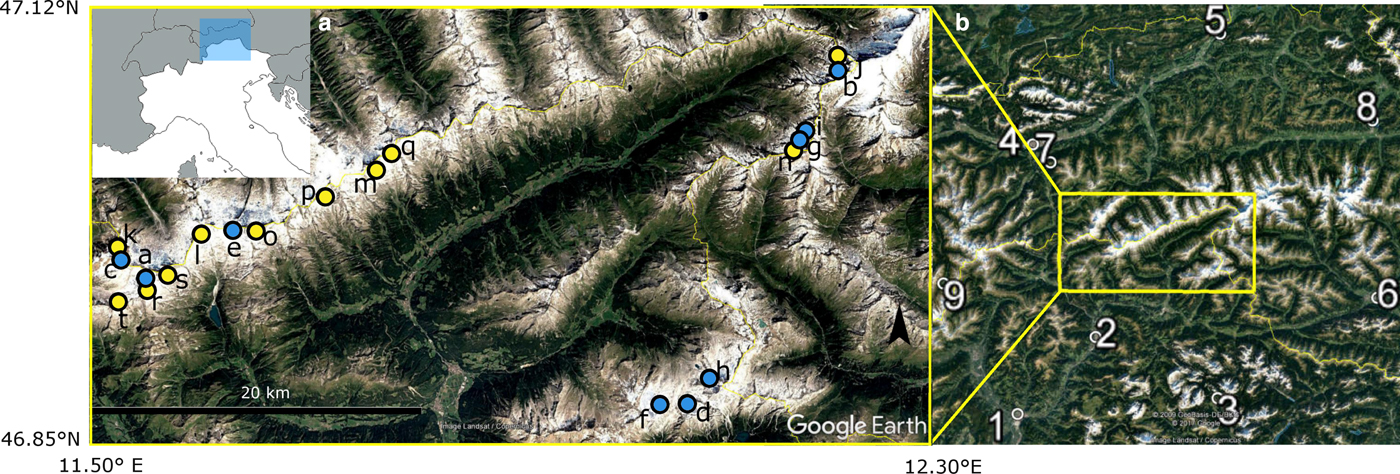
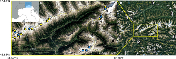
Fig. 1. The Italian Western Tauri (Eastern Alps). Panel a: locations of the studied glaciers (blue dots, a--i in Table 1; yellow dots, j--t in Table 2). Panel b: locations of the climatic stations 1 Bozen/Bolzano, 2 Brixen/Bressanone, 3 Cortina d'Ampezzo, 4 Innsbruck University, 5 Kufstein, 6 Lienz, 7 Patscherkofel, 8 Zell am See and 9 Obergurgl-Vent.
Table 1. Area A, length L and slope α of the nine measured glaciers of the Western Tauri.

ID codes refer to the Italian Glacier Inventory (Consiglio Nazionale delle Ricerche – Comitato Glaciologico Italiano, 1959–1962). Areas and lengths have been collected from the WGI in 1982. Areas in 2008 are from Smiraglia and Diolaiuti (Reference Smiraglia and Diolaiuti2015). The lengths in 2015 have been obtained from field measurements (Comitato Glaciologico Italiano, 1981–2016) starting from 1982 lengths. α is the angle between the glacier surface and the horizon. a--i refer to the glacier locations in Figure 1, panel a. The glaciers are reported in order of decreasing length;  ${\rm v}={\rm valley} \ {\rm glacier}$, ${\rm m}={\rm mountain} \ {\rm glacier}$.
Table 2. Area A, length L and slope α of the selected unmeasured mountain glaciers reported in order of decreasing length.
ID codes refer to Consiglio Nazionale delle Ricerche – Comitato Glaciologico Italiano (1959–1962). Areas, and length have been derived from data collected for WGI in 1982. Areas in 2008 are from Smiraglia and Diolaiuti (Reference Smiraglia and Diolaiuti2015). j--t refer to the glacier locations in Figure 1, panel a. α is the angle between the glacier surface and the horizon.
Among the glaciers without any front variation measurement (hereafter the unmeasured glaciers), all belonging to the mountain glacier type, only those with an area decrease not exceeding 50% between 1982 and 2008, have been selected. This threshold is an a priori choice to respect the condition for the application of the linear model, i.e., glacier length variations much smaller than mean length (see Eqn (5)). As a consequence of this threshold, 11 glaciers have been considered (Table 2; Fig. 1, panel a). In 1982, the lengths of these 11 glaciers ranged between 1800 and 700 m and their areas between 1.4 and 0.2 km2; their surface loss in 2008 varied between 21 and 48%, with greater fractional area losses for the glaciers shorter than or equal to 1 km.
2.2. The meteorological data
The glacier length fluctuations are driven by changes in temperature and precipitation; generally, temperature plays a predominant role (Mackintosh and others, Reference Mackintosh, Dugmore and Hubbard2002; Giesen and Oerlemans, Reference Giesen and Oerlemans2010). In this work, we use the air temperature data from nine stations (Fig. 1, panel b) obtained from the HISTorical instrumental climatology surface time series of the greater ALPine region (HISTALP, http://www.zamg.ac.at/histalp/). The stations are located within a distance of 100 kms around the study area, and their elevations range from 272 to 2247 m.
At the mid-latitudes, glacier behaviour is controlled by the sequence accumulation-ablation seasons that define the hydrological year. The mean annual temperature variations have been obtained by averaging the annual temperature fluctuations at the nine stations over the hydrological year, from October to September. This average attenuates potential spurious oscillations which may be present in a single station time series. Figure 2 reports the temperature fluctuations along with their 11-year moving average which is used in this paper as a reference for the model validation. The choice of the 11-year moving average resulted from a trade-off between the need to preserve the long-time variations of the signal and to omit the oscillations with periods shorter than 5 years. Linear regressions of the filtered signal from 1930 to 2015 and from 1980 to 2015 yield temperature increases of 1.8 and 1.5°C, respectively.
Fig. 2. The temperature fluctuations derived by averaging the time series at the stations listed in Figure 1. The bold line is the 11-year moving average.
Because of the high variability of precipitation and the strong influence of orography, we have used precipitation data from the Bressanone station (#2 in Fig. 1, panel b), the closest to the considered glaciers. Annual and winter precipitation amounts (accumulation season), expressed in mm of water equivalent, do not show any trend over the period 1930–2015, but rather long-term oscillations are evident in the 11-year moving average curve (Fig. 3).
Fig. 3. The annual and winter total precipitation between 1930 and 2015 in Bressanone, Italy, expressed in mm of water equivalent (w.e.). The dashed lines represent the 11-year moving averages.
3. THE MODEL
The model proposed by Leclercq and Oerlemans (Reference Leclercq and Oerlemans2012) estimates the air temperature T′m(t) fluctuations from the glacier length fluctuations L′(t), i.e.,
 $$ T'_{\rm m} (t) = - (L' (t) + \tau {\rm d}L' (t)/{\rm d}t) /C_{\rm s} $$
where L′(t) (m) is the variation in the glacier length with respect to its average value, dL′(t)/dt (m a−1) is the glacier variation rate, C s is the climate sensitivity (m K−1) and τ is the glacier response time (year). The climate sensitivity C s is defined as
 $$ C_{\rm s} = (\overline{P}_{\rm ann})^{\rm 1/2} / (c1\, \ast \, s) $$
where  $\overline {P}_ {\rm ann}$ (m a−1) is the mean annual precipitation at the glacier site and s is the glacier slope. The response time τ is
 $$ \tau = c_2 / (\beta s (1 + 20s)^{\rm 1/2} L^{\rm 1/2} ) $$
where  $\beta =c_3(\overline {P}_ {\rm ann})^ {\rm 1/2}$ (a−1m−1/2) is the balance gradient with the constant c 3 = 0.006 obtained from calibration with numerical simulations (Oerlemans, Reference Oerlemans2005). The constants c 1 = 0.0078 ± 0.0004 and c 2 = 1.35 ± 0.14 result from a re-calibration carried out by Zecchetto and others (Reference Zecchetto, Serandrei-Barbero and Donnici2017); this step is necessary because when the original coefficients are used, the temperature fluctuations produced by the model do not reproduce those from the observations. According to Leclercq and Oerlemans (Reference Leclercq and Oerlemans2012), the response time τ is defined as the time the glacier requires to reach (1-e−1) of the final length change after a stepwise perturbation of the climatic forcing. τ is also defined in Christian and others (Reference Christian, Koutnik and Roe2018) as the glacier response time-scale.
Equation (1) is a linear differential equation, which may be solved as
 $$ L'_{\rm m} (t) = - (1-{\rm e}^{-t/\tau}) C_{\rm s}T' $$
for an initial condition L′(t=0) = 0 and C s and T ′ constant. This equation provides the glacier length fluctuations  $ L^{'}_{\scriptscriptstyle \rm m}$ once the temperature variations T ′ are known. This solution is time dependent and describes the system in equilibrium at t = ∞; i.e., the glacier's response to a change in the temperature forcing would take an infinite time to reach a new equilibrium. The equation $L^{'}_{\scriptscriptstyle \rm m} (\infty )=C_{\rm s}T^{'} $ is therefore valid for equilibrium conditions, which are never reached. For t = 2τ the equilibrium is approached with 69% and Eqn (4) provides the value of $L^{'}_{\scriptscriptstyle \rm m}$ at this percent of equilibrium.
The model can be used provided the following condition (Oerlemans, Reference Oerlemans2011; Leclercq and Oerlemans, Reference Leclercq and Oerlemans2012) is respected
 $$ \sigma_{L}/L_0 \ll 1 $$
where σL is the standard deviation of the glacier length and L 0 is the glacier length (or mean) over the period considered. This condition states that the model can be applied only if the glacier variations are small with respect to its length; thus, implicitly, the model does not account for all the non-linear and local factors influencing a glacier's life, such as fragmentation and the consequent decoupling of length variations from the local temperature. Neither does the model account for changes in ice flow or debris cover. The results provided in this paper are all compatible with Eqn (5), and all the conclusions reached must be viewed in light of this constraint.
Both Eqns (1) and (4) need, as input, continuous and smoothed time series of L ′ and T ′, respectively. The time series of the glacier fluctuations with missing data have been interpolated using a shape-preserving cubic interpolation and then filtered using the Butter low-pass filter with a cutoff period of 15 years. The time series of T ′ have been smoothed with an 11-year moving average.
In the following sections, we use the term mean temperature (length) anomaly to refer to the quantity  $ \langle T^{'} - \overline { T^{'}} \rangle (t)$ (or L ′), where the overline indicates the mean over time and 〈〉 the average over the glacier length. The superscripts M and V refer to mountain and valley glaciers respectively. Thus, all the time series of each kind $\langle T^{'}_{\scriptscriptstyle \rm m} \rangle (t)$ have a null mean.
The model has been applied to small mountain and valley glaciers over the period 1980–2015 to evaluate its performance and over the period 2015–2100 to estimate the glaciers' life expectancies.
4. THE MODEL APPLIED TO THE MOUNTAIN GLACIERS
In this section, we test the performance of the linear model when applied to the small mountain glaciers over the period 1980-2015 in two ways: by assessing the temperature anomaly and by evaluating the relative snout position.
To perform the first test, we rely only on the measured mountain glaciers (Table 1), since we need the observed glacier snout variations to obtain the temperature fluctuations (Eqn (1)). For the second test, we use all the mountain glaciers available, both measured and unmeasured, since the forcing of the model is the temperature (Eqn (4)). These reconstructions do not include the Quaira Bianca (889) and Eastern Neves (902) glaciers, since they were used for the calibration of c 1 and c 2 (Eqns (2) and (3)) (Zecchetto and others, Reference Zecchetto, Serandrei-Barbero and Donnici2017). As reported in the model description, the model can be applied only to the glaciers that satisfy Eqn (5). While for the four measured mountain glaciers, σL/L satisfies this condition, for the unmeasured glaciers, the ratio is unknown. Therefore, Eqn (5) must be verified a posteriori from the model estimate of L m. For these glaciers,  $ \sigma _{\scriptscriptstyle L_{\rm m}}/{L_{\scriptscriptstyle \rm m}}$ has been estimated over running windows of 15 years showing that only for the six longest unmeasured glaciers (Table 2) is Eqn (5) satisfied.
The result of the first test is provided in Figure 4: it presents the model mean temperature anomaly  $\langle T^{'}_{\scriptscriptstyle \rm m} \rangle (t)$ (solid bold line) as function of time (t), obtained for the mountain glaciers $\langle T^{'{\scriptscriptstyle \rm M}}_{\scriptscriptstyle \rm m} \rangle (t)$ (solid line) and the valley glaciers $\langle T^{'{\scriptscriptstyle V}}_{\scriptscriptstyle \rm m} \rangle (t)$ (dotted line), along with the observed mean temperature anomaly $\langle T^{'}_{\scriptscriptstyle hy} \rangle (t)$ (dashed line). The error bars on $\langle T^{'{\scriptscriptstyle \rm M}}_{\scriptscriptstyle \rm m} \rangle (t)$ represent the standard deviation of the temperature fluctuations derived by the model for the four measured mountain glaciers, while the standard deviations $\langle T^{'}_{\scriptscriptstyle hy} \rangle (t)$ are based on the temperature fluctuations measured at the different meteorological stations. After 2010, the model mean temperature for the mountain glaciers has not been derived for lack of suitable data. The modelled temperature increase of ~ 1.7°C agrees with the general trend exhibited by the temperatures used in this study. Therefore, it seems reasonable that the model can also be used for the mountain glaciers.
Fig. 4. The temperature anomaly  $\langle T^{'{\scriptscriptstyle \rm M}}_{\scriptscriptstyle \rm m} \rangle (t)$ for the measured mountain glaciers (solid line) along with the observed temperature anomaly $\langle T^{'}_{\scriptscriptstyle hy} \rangle (t)$ (dashed line) and the mean model temperature anomaly $\langle T^{'}_{\scriptscriptstyle \rm m} \rangle (t)$. $\langle T^{'{\scriptscriptstyle V}}_{\scriptscriptstyle \rm m} \rangle (t)$ for the valley glaciers (dotted line) is reported for reference.
The second test was carried out by using the mean air temperature as presented in (Fig. 2) and Eqn (4) with t = 2τ. Figure 5 reports the mean model results for all (measured and unmeasured) mountain glaciers  $\langle L^{'{\scriptscriptstyle M}}_{\scriptscriptstyle \rm m} \rangle (t)$, with the mean 〈L ′〉(t) for the measured mountain glaciers and the $\langle L^{'{\scriptscriptstyle V}}_{\scriptscriptstyle \rm m} \rangle (t)$ of the valley glaciers for reference. The average length retreat of 333 m provided by the model for the valley glaciers is consistent with the observed average length retreat of 365 m and with the mean climate sensitivity 〈C s〉 of 238 m K−1 (Table 3).

Fig. 5. The model glacier mean length anomaly  $\langle L^{'{\scriptscriptstyle M}}_{\scriptscriptstyle \rm m} \rangle $ for the mountain glaciers (bold solid line). Dashed line: 〈L ′〉(t) obtained from in situ measurements related to the four measured mountain glaciers. Solid line: $\langle L^{'{\scriptscriptstyle V}}_{\scriptscriptstyle \rm m} \rangle (t)$ for the valley glaciers.
Table 3. The model results for valley and mountain glaciers.
The mean of the modelled length fluctuations of the mountain glaciers  $\langle L^{'{\scriptscriptstyle M}}_{\scriptscriptstyle \rm m} \rangle (t)$ lies between those of the valley $\langle L^{'{\scriptscriptstyle V}}_{\scriptscriptstyle \rm m} \rangle (t)$ and the observed 〈L ′〉(t) fluctuations. For the six longest unmeasured glaciers, the average area loss from 1982 to 2008 is ~34%. For the measured mountain glaciers, a 39% loss of area corresponds to a mean length decrease of 25%. Since measured and unmeasured mountain glaciers pertain to the same glacier type and have similar sizes, a similar length reduction for the unmeasured glaciers is expected: the model results (Table 3) indicate length reductions between 12 and 32%. The mean modelled length reduction of the four measured mountain glaciers $\langle L^{'{\scriptscriptstyle M}}_{\scriptscriptstyle \rm m} \rangle $ (491 m) is comparable with their mean observed retreat 〈L ′〉 of 477 m. The mean climate sensitivity 〈C s〉 of all mountain glaciers, measured and unmeasured, is 290 m K−1.
The results of the comparison between the model and the observations in the past (1980–2015) indicate that the model is sufficiently reliable to be used for future projections forced by climatological temperatures.
5. GLACIER LIFE EXPECTANCY
To investigate a glacier's future behaviour under the global warming scenario, we have used the temperature projections of the A1B emission scenario, which ….describes a future world of very rapid economic growth, global population that peaks in mid-century and declines thereafter, and the rapid introduction of new and more efficient technologies (Nakićenović and others, Reference Nakićenović2000). In particular, the A1B scenario is derived under a supposed balance of fossil intensive and non-fossil energy sources.
In the Alps, the A1B scenario indicates a temperature increase of 0.25°C per decade until the mid of the 21st century and of 0.36°C per decade in the second half of the century, i.e., 2.7°C from 2015 to 2100. These temperature projections have been used by Gobiet and others (Reference Gobiet2014) to analyse future climate change in the European Alps. This temperature projection is more severe than the intermediate RCP4.5 scenario (emissions peak around 2040, then decline), which for the Tyrol area reports an increase of 2°C at the end of this century, and less severe than the RCP8.5 scenario (business-as-usual), which indicates an increase of 4.6°C for Tyrol (IPCC, Reference Pachauri and Meyer2014; Chimani and others, Reference Chimani2017). The temperature increase from 2015 to 2100 from the A1B scenario described above is plotted in Fig. 6 (solid and dotted lines), where the observed temperature variations from 1980 to 2015 are added for reference (dashed line). The presented scenario is used as forcing in Eqn (4) to derive the climatological glacier length variations.
Fig. 6. The climatological forcing temperature anomaly used to estimate the future changes in glaciers. Solid and dotted lines: projections derived from the A1B scenario until and after 2050, respectively (Nakićenović and others, Reference Nakićenović2000). The observed temperature variations from 1980 to 2015 (dashed line) are reported for reference. The vertical line indicates the start time for the computation of the climatological glacier length variations.
As noted above, Eqn (5) must be satisfied to consider the model's results reliable. Of course, the ratio σL/L is not known for the future; therefore, it has been obtained from the model estimate of L m over running windows of 15 years, and Eqn (5) has been verified a posteriori. Fig. 7a presents the model-derived  $ \sigma _{\scriptscriptstyle L_{\rm m}}/{L_{\scriptscriptstyle \rm m}}$ as a function of time for the period 2015–2100 and all glaciers considered. For two glaciers, the West Ries (930) and East Central Ries (929), the model is applicable only until the 2050s, while for the other glaciers, the model is applicable until the end of this century.
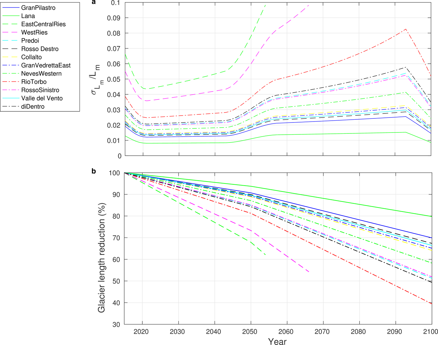
Fig. 7. The changes in valley and mountain glacier lengths obtained using the temperature scenario as presented in Figure 6. Panel a: model-derived  $ \sigma _{\scriptscriptstyle L_{\rm m}}/{L_{\scriptscriptstyle \rm m}} (t)$ as a function of time. Panel b: percentage of the glacier length variations as a function of time. Valley glaciers: solid lines; measured mountain glaciers: dashed lines; unmeasured mountain glaciers: dotted lines. The legend denotes the names of the glaciers in order of decreasing length.
Figure 7b reports the glacier length variations as a function of time for the periods of applicability of the linear model given by Eqn (4) and depicted in Fig. 7a. These results show the retreat of the glaciers until they behave linearly, in other words, until the Eqn (5) is satisfied. Otherwise, the linear model cannot be used because highly nonlinear processes of glacier decay are dominant. The length decreases for the valley glaciers (solid lines) are less than those for the mountain glaciers (dashed lines). For two mountain glaciers, the condition of applicability of the linear model holds only until 2055 (East Central Ries glacier) and 2066 (West Ries glacier). These glaciers show retreats of ~40% by 2060.
By the end of this century, the total length retreat is estimated to be from 20 to 60%, with expected length reductions of 20--35% for valley glaciers and of 35--60% for mountain glaciers with length > 1 km.
6. DISCUSSION
For the glaciers of the Swiss Alps, Huss and Fischer (Reference Huss and Fischer2016), based on glaciers smaller than 0.5 km2 and climate scenarios A1B, A2, RCP3PD, estimated that 71% of the glaciers will have disappeared by 2040. The lifespan of the Western Tauri glaciers (0.01–1.93 km2), based on the length reductions expected by 2100 under climate scenario A1B, seems higher than the life expectancy predicted for the Swiss Alps glaciers. Furthermore, as shown in Table 1, a decrease in length of 10--34% over the period 1982–2015 corresponds to a surface area reduction of 25--55%. The modelled length reductions of 35--60% of the mountain glaciers with length > 1 km by the end of the century (Fig. 7b) can therefore be the result of surface area reductions >60%. For mountain glaciers with lengths ≤ 1 km, surface area reductions far >60% are expected. These area losses lead to a general fragmentation into smaller units with consequent acceleration of the retreat rate, given the positive feedback due to thermal radiation from now ice-free terrain observed at the snout of some glaciers (Comitato Glaciologico Italiano, 1981–2016) and to the decrease in glacier albedo caused by several years with negative mass balance (Paul and others, Reference Paul, Machguth and Kääb2005; Haeberli and others, Reference Haeberli, Hoelzle, Paul and Zemp2007). The expected length reduction obtained from the linear model (Fig. 7b) also shows that valley glaciers with reductions of 20--35% have the highest life expectancy.
To achieve an overall assessment of the length reduction of the Western Tauri glaciers, the 26 glaciers so far excluded because their area losses exceed 50% between 1982 and 2008 must also be considered. In this time interval, these glaciers underwent a mean surface retreat of 61% with an area reduction up to 90%. These glaciers represent the following types: glaciers with surface areas between 0.05 and 1 km2 in 1982, now < 0.05 km2 (5 glaciers); glaciers with surface reductions of 60--90% over the period 1982 to 2008 (23 glaciers); and/or glaciers already fragmented in 2008 (14 glaciers) by the positive feedback due to thermal radiation derived from now ice-free rock outcrops. Among these 26 glaciers, none is in the potentially favourable situation to be avalanche-fed at sites that are radiation-protected and at low elevation and thus sensitive to increasing winter precipitation. The interaction of these negative feedbacks described by Huss and Fischer (Reference Huss and Fischer2016) for the Swiss Alps, by Colucci (Reference Colucci2016) and Carturan and others (Reference Carturan2013a) in the Julian Alps and by DeBeer and Sharp (Reference DeBeer and Sharp2009) for the Monashee Mountains (Canada) counteracts the glacier decay. Although almost all presented glaciers are avalanche-fed, the southern exposure makes the survival of some of these glaciers impossible. For other glaciers, such as the Cima Dura glacier (between glaciers f and m in Fig. 1), even though they are avalanche-fed glaciers located at low elevations in radiation-protected northern locations, they are already fragmented into smaller ice bodies and subjected to rapid disintegration (Treyer, Reference Treyer2012). A length reduction more severe than that presented in Fig. 7 is thus likely for these 26 glaciers, and they could be considered already disappearing.
Since 1982, the total area loss for the Western Tauri glaciers is 40%. From 1987 to the 2000s, in the nearby Ortles-Cevedale group, only 23% of the glacierized area was lost: this minor reduction seems due to the widespread negative feedbacks on glacier wastage observed in this glacier system, such as an increase in debris cover and a decrease in clear-sky radiation during summer, due to increased topographic shading (Carturan and others, Reference Carturan2013b). The 40% shrinkage observed for the Western Tauri glaciers agrees with the 48% recorded in the Western Alps by Nigrelli and others (Reference Nigrelli, Lucchesi, Bertotto, Fioraso and Chiarle2015) for the same period. Compared with the 13% area loss from the 1930s to 1960s, the measured decline confirms the current historically unprecedented glacier shrinkage (Haeberli and others, Reference Haeberli, Hoelzle, Paul and Zemp2007; Paul and others, Reference Paul, Kääb and Haeberli2007; Zemp and others, Reference Zemp2015). With some exceptions, the observed reductions are inversely proportional to size in accordance with previous observations on other glaciers in the Alps (Serandrei-Barbero and others, Reference Serandrei-Barbero, Rabagliati, Binaghi and Rampini1999; Paul and others, Reference Paul, Kääb, Maisch, Kellenberger and Haeberli2004, Reference Paul, Frey and Le Bris2011; Diolaiuti and others, Reference Diolaiuti, Bocchiola, Vagliasindi, D'Agata and Smiraglia2012); therefore, an even faster glacial area loss is expected.
The glacier geometry (slope and length) represents the main factor controlling the glacier tongue reaction (Hoelzle and others, Reference Hoelzle, Haeberli, Dischl and Peschke2003) and defines the climate sensitivity C s and response time τ (Eqns (2) and (3)). On the 169 glaciers analysed by Oerlemans (Reference Oerlemans2005) in different regions of the world, τ ranges from 10 years for the steepest glaciers to a few hundreds of years for the largest glaciers with smaller slopes; C s is between 1000 m K−1 and 10000 m K−1. On the northern side of the Eastern Alps (Oerlemans, Reference Oerlemans2007, Reference Oerlemans2012), the Vadret da Morteratch and Hintereisferner glaciers, both ~7 km long, have τ ≈ 33 years; Kesselwandferner and Vadret da Palü glaciers, ~4 km long and steeper, have τ from 2 to 4 years. On the Italian side of the Eastern Alps, the value of τ for three valley glaciers with lengths between 3 and 1 km is ~3--4 years, and the resulting C s is between 174 and 234 m K−1 (Zecchetto and others, Reference Zecchetto, Serandrei-Barbero and Donnici2017). For the mountain and valley glaciers considered in this study, with lengths between 3 and 0.7 km, the mean value of C s (278 m K−1) is consistent with the ground data, and τ between 3 and 20 years agrees with other values observed in the Alps, which are generally between 10 and 20 years (Paul and others, Reference Paul, Kääb, Maisch, Kellenberger and Haeberli2004).
On the mountain glaciers, 〈C s〉 is 290 m K−1 with a large spread for individual glaciers. The exceptionally high C s values of the Eastern-central Ries (929) and the Western Ries (930) glaciers (Table 3) are due to their gentle slopes and their elevations not exceeding 3000 m a.s.l. This situation implies that these glaciers are located below the current equilibrium line altitude, estimated at ~3100 m on glaciers belonging to the Adige River basin (Zemp and others, Reference Zemp, Hoelzle and Haeberli2007). Apart from these two most gently sloping glaciers whose τ is between 11 and 20 years, all the other have τ from 3 to 6 years.
On the valley glaciers, the results show less variability since larger glaciers generally tend to have gentler slopes (Paul and others, Reference Paul, Frey and Le Bris2011; Oerlemans, Reference Oerlemans2012); the highest C s value is 359 m K−1 for the largest glacier (Gran Pilastro, 893), and the lowest value is 143 m K−1 for the Valle del Vento (919) glacier, the smallest among the considered valley glaciers (Table 3). The ground surveys agree with these results: between 1980 and 2015, the average retreat rate of the Valle del Vento glacier was less than half the retreat rates of Gran Pilastro and Lana glaciers (Comitato Glaciologico Italiano, 1981–2016). These results of the linear model favour a longer survival for valley glaciers (Fig. 7b) and agree with the theoretical analyses of Bahr and others (Reference Bahr, Pfeffer, Sassolas and Meier1998) and Pfeffer and others (Reference Pfeffer, Sassolas, Bahr and Meier1998) which show that for the same climatic conditions, larger valley glaciers respond faster than smaller glaciers to perturbations in mass balance. This outcome occurs because larger valley glaciers push farther into the ablation zone.
In the present retreat phase, the primary classification appears ephemeral and somewhat subjective as the valley tongue is the most vulnerable and rapidly perishable glacier part (Carturan and others, Reference Carturan2013b). In this regard, the Rosso Destro glacier is today a mountain apron glacier (Cogley and others, Reference Cogley2011) while in contrast, the Lana and Valle del Vento glaciers are classified as mountain glaciers (Smiraglia and Diolaiuti, Reference Smiraglia and Diolaiuti2015), despite the fact that they still have evident valley tongues (Fig. 8). Despite the limits of the primary classification (Paul and others, Reference Paul2009), the glacial morphology seems to be a possible discriminating factor of a glacier's response to climate variations, and only the valley glaciers seem expected to survive beyond the end of this century, even though they belong to the same dimensional classes as the mountain glaciers such as the Valle del Vento glacier.
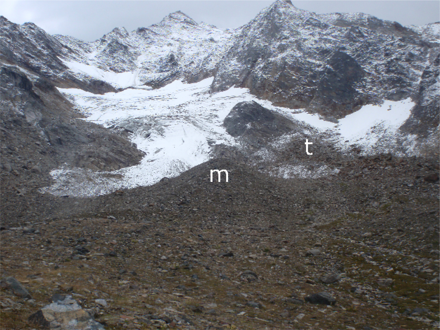
Fig. 8. The Valle del Vento (919) glacier in 2015. The medial moraine m is located at the confluence of the two ablation tongues dating back to the Little Ice Age. The left tongue t is now extinct, and the right terminus is hidden by debris cover, present only on the snout.
7. CONCLUSIONS
In this work, we used a linear model to analyse the future changes in the Italian Western Tauri glaciers until 2100, forced by temperature increases according to the A1B scenario, as used before in the Alps by Gobiet and others (Reference Gobiet2014). To date, the model has generally been used for valley glaciers, but in this study, it was tested on small mountain type glaciers for the period between 1980 and 2015; then, it was also applied to unmeasured glaciers located in this area.
The comparison between the model results and the observations indicates that the model is sufficiently reliable to be used for future projections forced by climatological temperatures. The model, using a mean sensitivity 〈C s〉 of 278 m K−1 and forced by a temperature increase of 1.5°C from 1980 to 2015, produces results consistent with the average frontal retreat of 462 m obtained from the in situ measurements. For valley glaciers, the retreat rate decreases with decreasing length, probably prolonging their life, while mountain glaciers, generally smaller than valley glaciers, are more exposed to the temperature increase, which probably condemns them to disappear within a few decades.
By 2100, the model projections indicate a shortening of 20--35% for 2015 valley glacier lengths (3135–975 m) and far more than 35% for the mountain glacier lengths (1997–819 m), resulting in an average area loss of more than 60%. This expected strong average reduction in area has to be considered a lower bound value since progressive glacier shrinkage and fragmentation will also lead to increasing glacier melt under the same climatic conditions given the delayed effects of temperature increase due to response time. Furthermore, the climatological scenario adopted is an intermediate type (similar to the RCP4.5 scenario), and other more severe scenarios are far more likely at present.
In the Italian Western Tauri, mountain glaciers represent ~95% of the glaciers. The projected large reduction of the modelled mountain glaciers by 2100 (> 60% of area loss), together with the vanishing already under way of the 26 smallest mountain glaciers not treated by the model, would mean the extinction of almost the totality of the existing glaciers by the end of this century, possibly leaving only three valley glaciers to survive.
ACKNOWLEDGMENTS
The glacier frontal variation data have been downloaded from the World Glacier Monitoring Service (www.wgms.ch), and the meteorological data, from the Historical Instrumental Climatological Surface Time Series Of The Greater Alpine Region (HISTALP) web site http://www.zamg.ac.at/histalp. The field measurements from 1982 to 2015 were supported by the Comitato Glaciologico Italiano. This work was partially funded by the Italian project of Interest NextData of the Italian Ministry for Education, University and Research.
We thank the scientific and associated chief editors, Carleen Tijm-Reijmer and Hester Jiskoot, the anonymous referee and Michael Kuhn for their efforts in reviewing the paper. David Winston revised the English in the manuscript.


 Open access