


1. INTRODUCTION
The ice cover in Greenland consists of the Greenland ice sheet (GrIS) and ~20 300 peripheral mountain glaciers and ice caps (MGIC) (Rastner and others, Reference Rastner2012). The surface area of the GrIS is ~20 times larger than that of all the MGIC combined (Rastner and others, Reference Rastner2012) while its volume is 170 times greater (Huss and Farinotti, Reference Huss and Farinotti2012; Morlighem and others, Reference Morlighem2017). Both GrIS and MGIC have been changing rapidly in recent decades (Bolch and others, Reference Bolch2013; Khan and others, Reference Khan2015; van den Broeke and others, Reference van den Broeke, Enderlin, Howat, Munneke and Noël2016). Around 41% of the current global land ice contribution to sea-level rise stems from the GrIS, while the MGIC contribute 7 ± 1% (Gardner and others, Reference Gardner2009; Box and Colgan, Reference Box and Colgan2017). Even though the absolute mass loss is larger from the GrIS than from the MGIC, the specific mass loss per unit area is smaller. Comparing van den Broeke and others (Reference van den Broeke, Enderlin, Howat, Munneke and Noël2016) and Noël and others (Reference Noël2017) shows that for a similar period, specific mass loss from MGIC is about four times higher than that from GrIS, underlining the higher sensitivity of MGIC mass balance to ongoing climate change. These studies also show that the uncertainties of mass change estimates of MGIC are about two times as large as the one for the GrIS.
Machguth and others (Reference Machguth2016) did a thorough compilation of existing mass-balance observations in Greenland and showed that in recent years the number of observations at the GrIS have increased tenfold. According to van As and others (Reference van As2011) the PROMICE project made an important contribution there. Particularly, the MGIC are heavily undersampled despite their complexity in mountainous terrain. To our knowledge, currently only six out of 20 300 MGIC are monitored in Greenland, three of which are at the West coast. Marcer and others (Reference Marcer2017) did a recent analysis of decadal changes of a mountain glacier in West Greenland and found a volume loss of 25% between 1985 and 2014. Yde and others (Reference Yde2014) investigated decadal ice volume changes on Mittivakkat Gletscher in East Greenland and found a volume reduction of 30% between 1994 and 2012 there. Very recently, von Albedyll and others (Reference von Albedyll, Machguth, Nussbaumer and Zemp2018) found a mean ice thinning of −0.24 m a−1 between 1978 and 2012–15 at Holm Land Ice Cap in North Greenland. These studies confirm high rates of MGIC mass loss and underline the importance to quantify their drivers.
Greenland is subject to strong climatic gradients and associated differences in energy input (Abermann and others, Reference Abermann2017). While latitudinal gradients are a consequence of the large north-south extent of the island, longitudinal gradients are mainly due to local effects such as increasing continentality moving from the coast to the ice sheet associated with variations in topography and large-scale moisture sources. Taurisano and others (Reference Taurisano, Bøggild, Karlsen and Boggild2004) elaborated on climate gradients in the Godthåbsfjord area and identified relationships between stations at coastal sea level with one at a similar latitude but higher altitude. More recently, Pedersen and others (Reference Pedersen2018) investigated both climate, snow cover and resulting gradients of vegetation growth in East Greenland based on remote sensing and model results. They emphasize that coast-to-inland gradients exceed the magnitude of latitudinal ones by far.
The term ‘glacier mass balance gradient’ is usually referred to as ‘the rate of change of mass balance with altitude’ on a specific glacier (Cogley and others, Reference Cogley2011). For this study, we define the ‘average horizontal surface mass balance gradients’ as the rate of change of mass balance with distance from the coast to the ice sheet at the same elevation.
The complexity of horizontal surface mass-balance gradients and their quantification in itself is scientifically relevant in order to reduce uncertainties in mass change estimates. It would benefit calculations of future mass loss when the mass balance of MGICs, which are difficult to resolve in climate models, can be parameterized and/or scaled to GrIS estimates. To parameterize these, potentially under changing conditions, a physical approach to assess the atmospheric drivers is necessary.
We present in this study a unique dataset of concurrent in situ observations of glacier mass balance and the atmospheric drivers at one coastal glacier covered site and two more continental ice-sheet sites in southwest Greenland. We use the data to quantify the average horizontal surface mass-balance gradients and identify the atmospheric forcing mechanisms.
2. STUDY SITE
Our study region is Southwest Greenland's Godthåbsfjord area, inland from Greenland's capital Nuuk (Fig. 1). As a near-coastal, more maritime site we use results from Qasigiannguit glacier (QASI; 64.16°N; 51.35°W) which is a small (0.7 km2) north-facing glacier situated on the north side of Kobbefjord, 18 km east of Nuuk. The glacier spans an elevation range 680–1000 m a.s.l. The QASI surface mass-balance program was initiated in the framework of the Greenland Ecosystem Monitoring (GEM) program (http://www.g-e-m.dk), in order to better understand the cryospheric component in a low-Arctic ecosystem. In 2014, an automated weather station (AWS) was established on the glacier at 710 m a.s.l. in collaboration with the programme for monitoring of the GrIS (PROMICE, http://www.promice.dk). Glacier cover in the area has recently been studied on millennial timescales by Larsen and others (Reference Larsen2017). They found that QASI glacier likely disappeared between ~8.7 and 1.6 ky BP. Its Little Ice Age maximum was ~1900 AD of which a moraine system is still present. Thereafter the glacier shortened and reduced mass significantly and likely continuously.
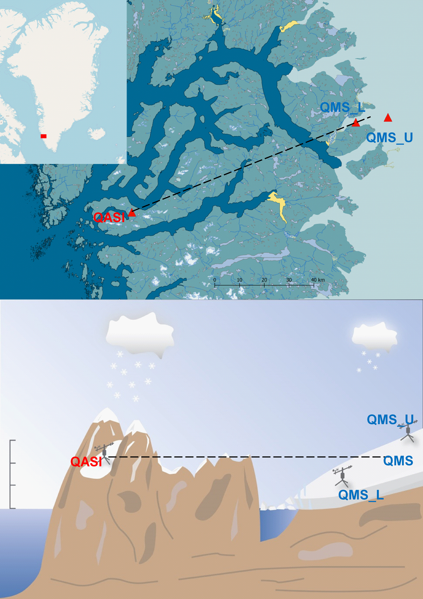
Fig. 1. The study area in southwest Greenland (upper panel) and a schematic sketch of the location of QASI vs. QMS (QMS_L and QMS_U). The distance between QASI and QMS is 103 km while the distance between QMS_L and QMS_U is 13 km.
As a more continental site on the ice-sheet margin we use the area of Qamanarssup Sermia, a land-terminating outlet glacier of the GrIS. The glacier is located ~100 km inland of QASI and is equipped with two AWS managed and maintained since 2007 by PROMICE. The lower station is referred to as QMS_L and is located at ~530 m a.s.l. (N64.48, W49.54). The second station QMS_U (N64.54, W49.27) is in the upper ablation zone at ~1120 m a.s.l. (Fig. 1 upper panel).
3. METHODS
Seasonal (winter and net) mass balance is measured at QASI with a stake network of 7–11 stakes that get revisited several times a year. The AWS QMS_L and QMS_U get visited once a year in summer, and net mass balance is derived by the recorded relative change of ice surface height using a pressure transducer (Fausto and others, Reference Fausto, As, Ahlstrøm and Citterio2012) and a volume-to-mass density conversion of 900 kg m−3 for ice.
Here we use AWS data covering the time period 27 July 2014–1 October 2016 with two data gaps: Due to heavy snow cover and covered sensors at QASI we did not use data from 21 March 2015 to 24 June 2015. Station failure at QMS_U between 01 November 2015 and 03 April 2016 led to another data gap. We use monthly averages of atmospheric variables for months during which all three AWS were operational. The averages presented are not gap-filled. The AWS at all sites are identical and a detailed description is given in Citterio and others (Reference Citterio2015).
The complexity of the area is shown schematically in Figure 1b, with additional difficulty caused by different measurement altitudes with the AWS on coastal site QASI at 710 m a.s.l. and the two AWS QMS_L at 530 and QMS_U at 1120 m a.s.l., respectively. In order to remove elevational discrepancies we interpolate the meteorological measurements from QMS_L and QMS_U linearly to an elevation of 710 m a.s.l., and refer to the interpolated time series (labelled QMS) in the remainder of the study. The horizontal distance between QASI and QMS (see Fig. 1) is 103 km, thus, the average horizontal surface mass-balance gradient can be derived as
 $$\displaystyle{{\Delta b} \over {\Delta x}} = \; \displaystyle{{b_{{\rm QMS}}-b_{{\rm QASI}}} \over {103}}\; \; \; \; [ {mm\; w.e.\,\,km^{-1}} ] $$
The surface radiation balance is defined as
 $$\; {\rm R_n} ={\rm S}{\rm W}_{{\rm in}}-\; {\rm S}{\rm W}_{{\rm out}} + {\rm L}{\rm W}_{{\rm in}}-\; {\rm L}{\rm W}_{{\rm out}}$$
Where R n is net radiation, SW is shortwave radiation, LW is longwave radiation, and the indexes ‘in’ and ‘out’ indicate incoming and outgoing components, respectively. The surface energy balance of the glacier surface is described as
 $$R_n + {\rm SH} + {\rm LH} + G + R = M.$$
where SH and LH are the nonradiative turbulent sensible and latent heat fluxes, respectively; G the conductive ground heat flux, R the energy added through rain and M the ‘residual’ or the energy available for melt of snow or ice. Energy input to the surface yields positive values, while negative values depict an energy loss. We compute the energy-balance components following van As (Reference Van As2011). Turbulent fluxes were calculated with the bulk method assuming Monin-Obukhov similarity theory. Aerodynamic surface roughness lengths for momentum over ice were set to 2 mm at QASI and QMS_U and 5 mm at QMS_L, and to 0.1 mm for snow for all sites. R is set to zero as it is assumed negligible compared with the magnitude of other fluxes.
4. RESULTS
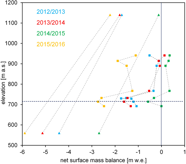
Net surface mass-balance values for Qamanarssup Sermia and Qasigiannguit glacier are shown in Figure 2 for the four mass-balance years between end-of-ablation-season 2012 and 2016. Each point refers to a surface mass-balance measurement at a stake or AWS location. Net-mass balance is generally less negative at QASI than at QMS. The interannual variability is high with several meters of water equivalent at the same elevation. For instance, at 710 m a.s.l. we find period-mean values of −1.5 and −3.7 m w.e. at QASI and QMS (Table 1), with large standard deviations of 0.9 and 1.2 m w.e., respectively. Interannual variability across sites follows the same pattern with 2014/15 being the most positive year, and 2015/16 the most negative year (Fig. 2, Table 1). The elevation for which we compare atmospheric parameters and energy-balance components (710 m a.s.l.) is in the ablation zone for all years.
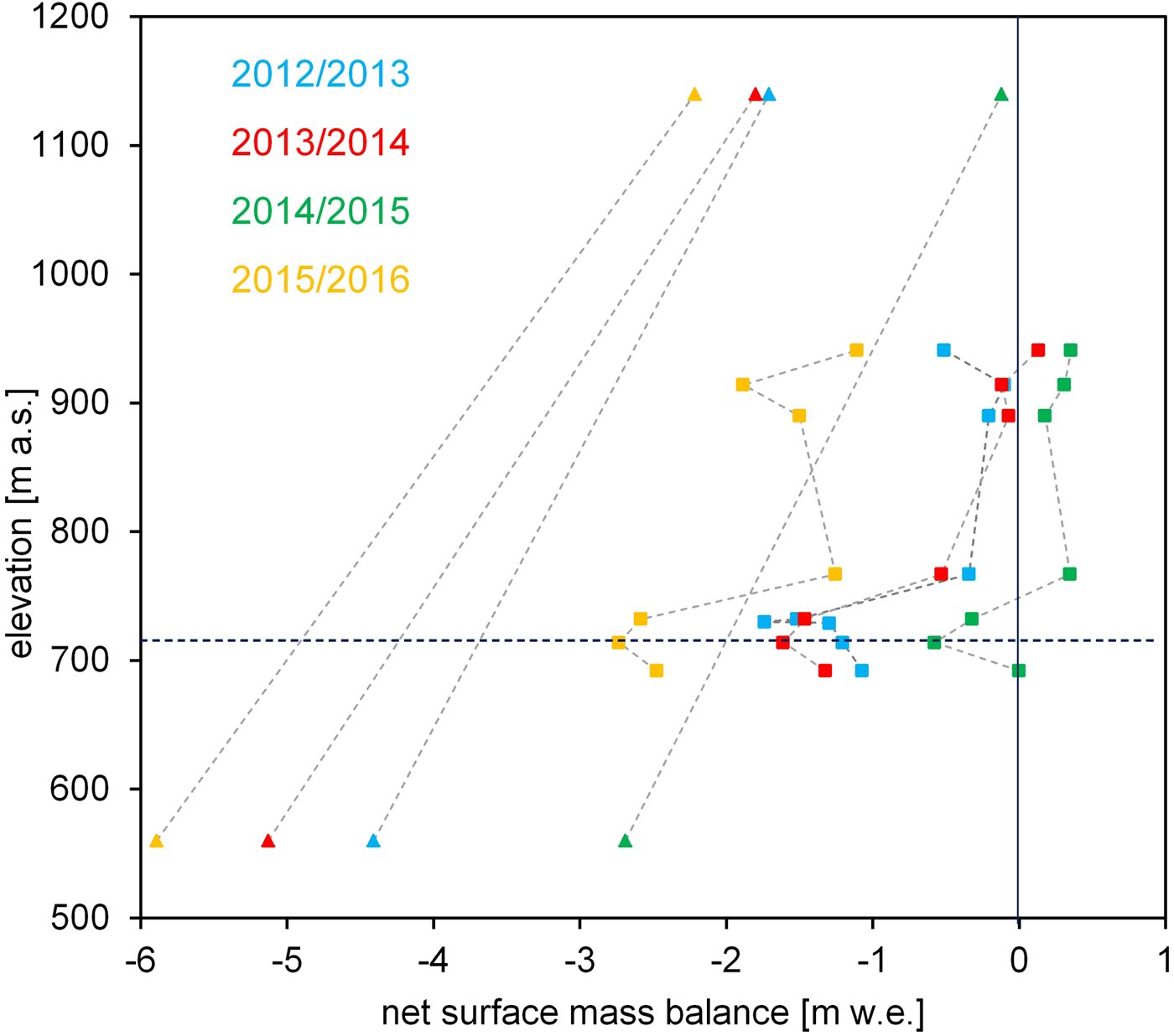
Fig. 2. Net mass balance at QMS_L and QMS_U on QMS (triangles) and at all available stakes at QASI (squares). Same colours mean the same year. The horizontal line shows the elevation of the AWS on QASI (710 m a.s.l.) and for which we perform the comparison.
Table 1. Specific net surface mass balance at QASI (b net QASI) and QMS (b net QMS), average horizontal net surface mass-balance gradient (dbnet/d x) and number of snow-free days at QASI derived from an automated camera overlooking the glacier and at QMS from the relative surface height change

Table 1 shows the net balance at QASI and QMS and the average horizontal net surface mass-balance gradients as derived using Eqn (1). Values vary between −20 and −30 mm w.e. km−1, meaning that on average with every km distance from the coast an additional 20–30 mm w.e. ablates each year at 710 m a.s.l.. Anomalies in winter and net mass balance at QASI indicate a relation with winter balance, where more positive winter balances indicate a weaker horizontal gradient.
Figure 3 shows monthly averages of selected atmospheric variables measured at the AWS at QASI and at QMS. For most of the year and particularly during summer months air temperature (AT) is slightly higher at QASI than at QMS (0.5 °C annual average, Table 2). ATs in spring are very similar (Fig. 3a). Relative humidity (Fig. 3b) is on annual average 10% higher at QASI (Table 2) with the biggest difference in March (20% more humid at QASI). Wind speeds are generally higher at QMS due to differences in katabatic forcing. This is true all year round but particularly strong during spring and early summer when stable weather at QASI yields low wind speeds. On average, wind speed is 1.3 m s−1 higher at QMS.

Fig. 3. Near-surface atmospheric variables measured at QASI (red) and at QMS (blue): (a) Air temperature, (b) relative humidity, and (c) wind speed.
Table 2. Average atmospheric variables, physical properties and surface energy-balance components on a total annual basis and for JJA only

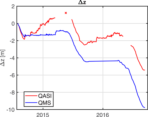
Continuously measured changes in relative surface height for the period July 2014 until 2016 are shown in Figure 4. Similar ablation rates are found at both sites during snow-free conditions, but marked differences in accumulation occur. While QASI receives up to 3 m of snow during the winter, QMS receives <1 m. The winter 2015/16 was particularly dry resulting in <1.5 m of accumulation at QASI and virtually no accumulation at QMS. The figure also shows the impact of snow on the length of the ice ablation season. During most of the spring and early summer the energy input on QASI is used to melt snow while ice ablation dominates over the same time period on QMS. The number of days with snow-free conditions was 53 and 64 days longer at QMS than at QASI in the summers of 2015 and 2016, respectively (Table 1).

Fig. 4. Surface elevation change due to accumulation and ablation at QASI and at QMS since July 2014. The sensor at QASI was covered by snow for parts of early 2015 due to heavy snowfall. The cross marks a manual measurement during a station visit.
The different components of the surface energy balance are shown in Figure 5. Ground heat flux (GF) typically contributes <10 W m−2 throughout the year and does not show a clear annual cycle. Latent heat fluxes (LH) do not exceed absolute values of 17 W m−2 during May on QMS. LH fluxes are on annual average 6 W m−2 more negative on QMS than on QASI, due to the generally drier air and higher wind speeds at QMS. Sensible heat (SH) input is positive throughout the year and almost four times higher at QMS than on QASI on annual average (Table 2). Maximum SH occurs during summer and can exceed 50 W m−2 as a monthly average on QMS. Longwave net radiation (LWnet) is negative throughout the year with larger negative values on QMS. For both sites LWnet is the largest energy sink and is on average 10 W m−2 lower on QMS than on QASI. On the other hand, short-wave net radiation (SWnet) is positive throughout the year at both sites and the largest energy source for most of the year. SWnet values are on annual average 13 W m−2 higher on QMS than on QASI. The maximum average SWnet is in July due to a darker ice surface and more stable weather than in June where QMS receives 52 W m−2 more radiation on average. During spring, differences between the sites are largest, with higher SWnet on QMS. The resulting energy balance (i.e. the sum of all components) shows that the availability of melt energy is largely determined by SWnet.
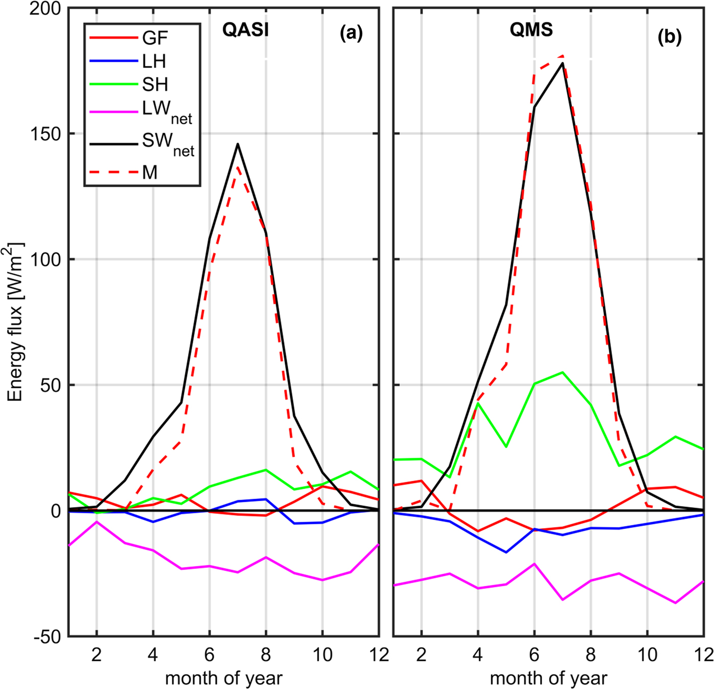
Fig. 5. Average monthly surface energy-balance components on QASI and QMS.
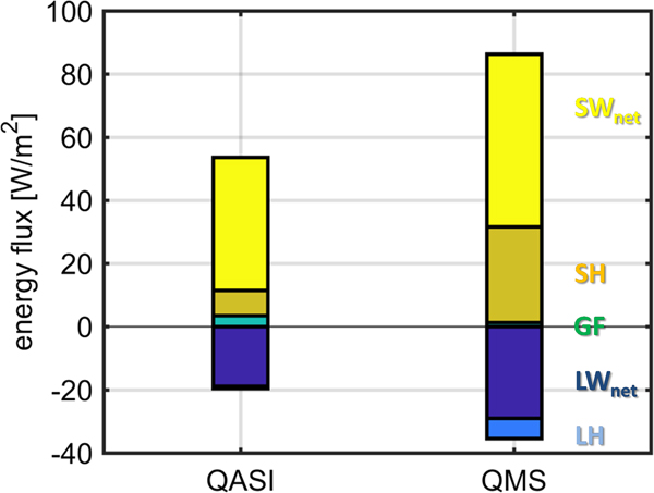
Calculating annual averages allows for ranking the relative importance of the energy-balance components (Fig. 6, Table 2). The two components with the largest absolute numbers are SWnet and LWnet. Both net radiative fluxes are of larger absolute magnitude on QMS. The turbulent fluxes are of opposite sign, too, however, the net turbulent heat flux contribution is positive at both sites. Generally, both energy input and output are larger on QMS than on QASI, leading to a higher energy turnover and ultimately to higher annual melt values. Ground heat flux plays a slightly larger role at QASI than at QMS but nevertheless is a minor energy-balance component. On annual average, 17 W m−2 more are available for melt at QMS compared with QASI (Table 2). In order to highlight the importance of the individual meteorological drivers and surface energy-balance components during summer, we report the respective values for June, July and August (JJA) in Table 2. During summer, the AT difference between QASI and QMS is approximately twice the difference of the annual average (1.1 /0.5 °C warmer on QASI than on QMS in summer /on annual average). Summer wind speed is lower than the annual average, but the difference between the sites is higher which leads to larger summer differences in SH due to stronger differences in AT. SWnet radiation is almost three times higher during summer than on annual average at both sites, which is a result of both higher incoming shortwave radiation and lower albedo during summer. Summer LWnet radiation is similar to the annual average.

Fig. 6. Annual averages of surface energy-balance components on QASI and on QMS.
5. DISCUSSION
Few other studies identified horizontal surface mass-balance gradients in Greenland based on measurements. Taking advantage of the data compiled in Machguth and others (Reference Machguth2016), we can estimate an average horizontal net mass-balance decrease between Qapiarfiup Sermia (65.58°N; 52.20°W) and Amitsuloq Ice cap (66.38°N; 50.88°W) of 11 mm w.e. km−1 at 950 m a.s.l. averaged over the 4 years between 1982 and 1984, and between 1987 and 1989. Ahlstrøm (Reference Ahlstrøm2003) derived equilibrium line altitude (ELA) gradients at the same sites and found that the ELA rises by 3.4 m km−1 when moving from the coast to the ice sheet. Since both stations on QMS are located in the ablation zone we are unable to compute ELA gradients based on our measurements. Close to the southern tip of Greenland at ~61°N, Clement (Reference Clement1983) measured a transect between Narssaq Bræ and Nordbogletscher and found an increase in equilibrium line altitude of ~450 m over the 94 km distance. The average net mass balance for the years with concurrent measurements (1980–82) at an elevation of 1150 m a.s.l. decreased from the coast inland by 15 mm w.e. km−1. Our values from Table 1 are on average by a factor of 1.4 higher.
The spatial representativeness of the differences in mass and energy balance from the coast to the ice sheet for other areas in Greenland is difficult to assess. Precipitation variability is high and the decrease from the ocean towards the continental part of the island occurs at all coastal stretches. In areas, with generally high precipitation, the differences are particularly large over short distances (e.g., Southeast Greenland, Burgess and others (Reference Burgess, Forster and Box2010)). The area in Southwest Greenland where our study is located is rather wet and hence likely shows above-average differences between the coast and the ice sheet. In Figure 7, we show that the elevation span of QASI (680–1000 m a.s.l.) embraces the areas at or below the median elevation of all MGIC in Greenland and hence shows a relevant part of the MGIC's ablation areas (Noël and others, Reference Noël2017). For the GrIS, the same elevation corresponds to the lower ablation zone and hence relatively stronger negative mass-balance values while the median elevation is much higher (Rastner and others, 2013).
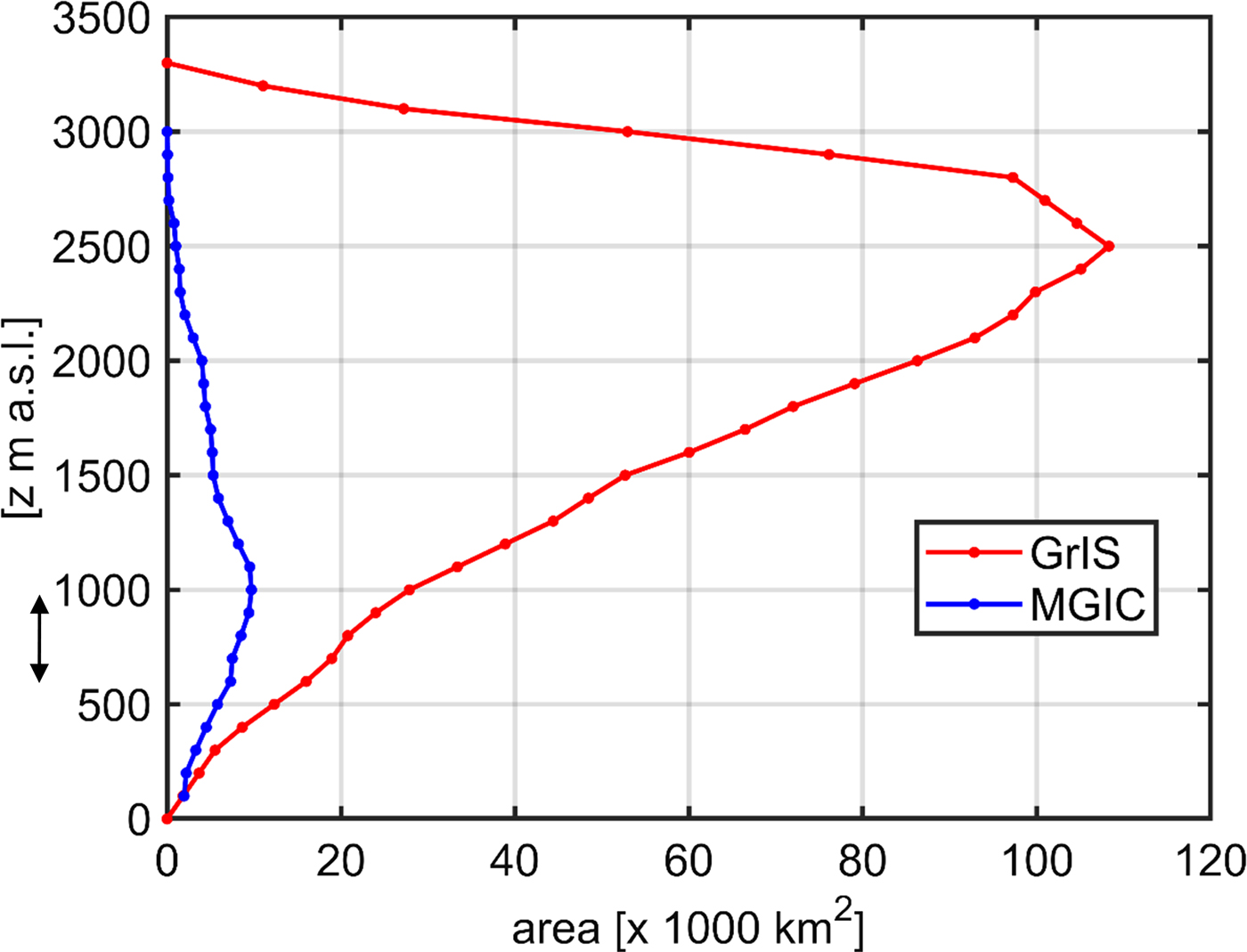
Fig. 7. Area-elevation distribution of the MGICs in Greenland (blue; data from Rastner and others (2010)) and the GrIS (red; data from Noël and others (Reference Noël2017)). Elevation bands covered by QASI are indicated with a black arrow.
Using the observed differences in meteorological variables and surface energy-balance components allows us to determine the drivers for the strong horizontal surface mass-balance gradients in our study. As shown in Figure 34, the coastal site QASI receives more accumulation because of its proximity to the ocean that is ice-free year-round and hence serves as a moisture source. Furthermore, the steep mountains close to the coast force precipitation orographically. This impacts the radiation fluxes in several ways. First, increased cloudiness reduces SWin. Second, more precipitation at QASI (Fig. 4) increases the length of the smooth, snow-covered, high-albedo period compared with QMS where the darker ice surface appears earlier. Third, clouds cause LWnet to be less negative, even more so at QASI than at QMS. Despite higher differences in energy available for melt during summer (45.0 W m−2 more on QMS than on QASI) compared with the annual mean (17.0 W m−2 more on QMS than on QASI), the fractional difference is higher averaged over the year (50% more energy at QMS compared with QASI averaged over the year; 39% averaged over the summer; Table 2).
The nonradiative turbulent fluxes have a smaller magnitude at QASI attributable to lower wind speeds (impacting both SH and LH) and higher atmospheric humidity (impacting LH). The relatively dry katabatic winds over the ice-sheet enhance turbulent mixing at QMS. ATs are slightly cooler at QMS than at QASI, which is likely related to the ‘glacier cooling effect’ as pointed out by Braithwaite (Reference Braithwaite1983), that is stronger on the large QMS. This AT difference does not sufficiently counteract the effect of the lower wind speeds in terms of SH exchange between atmosphere and surface. This illustrates the danger of oversimplified melt-model approaches based solely on ATs that would in our case result in a wrong sign of horizontal surface mass-balance gradients.
The average horizontal gradients in glacier surface mass balance vary from year to year and appear to be related to anomalies in accumulation. The weakest gradient was observed in 2014/15 (Table 1), the year with the least negative mass balance observed. A smaller difference between the number of snow-free days at QASI and at QMS than in the other years of our study period resulted in a shorter period with large albedo differences between the sites, reducing the average horizontal surface mass-balance gradient. It remains to be tested whether the observed relation also persists when analyzing a longer time series in the future. Since we do not have more comprehensive information we assume a linear vertical mass-balance gradient between QMS_L and QMS_U. This is likely oversimplified and historical data from the 1980s illustrate that there is a slightly inverted mass-balance profile between 600 and 800 m on QMS (Machguth and others (Reference Machguth2016): Fig. 6; Braithwaite and Olesen (Reference Braithwaite and Olesen1989)), however, the deviation from a linear profile is small compared with the horizontal gradient we observe which is why we consider this a minor issue.
Horizontal mass and energy-balance gradients likely do not occur linearly, which is why we emphasize that Eqn (1) and the numbers in Table 1 are average values. In reality, we assume the average value to be a combination of stronger changes near the coast where precipitation gradients are strongest and weaker changes closer to the ice sheet. In order to resolve this, high-resolution modeling would be an interesting approach; this is however, beyond the scope of this paper. Another limitation of Δb/Δx is the fact that the ice cover between QASI and QMS is discontinuous. We argue that for both reasons mentioned above, the numbers for Δb/Δx should only be used to compare differences in mass and energy balance over distances of similar orders of magnitudes rather than to derive a single glacier's mass or energy-balance value.
The observed differences in mass and energy balance are strongly related to variations in accumulation and atmospheric moisture. The difference in radiation balance between QASI and QMS indicates different conditions of cloudiness at the respective sites. It has recently been stated that the presence of clouds reduces refreezing and thus increases runoff from the GrIS (van Tricht and others, Reference van Tricht2016). In another study, Noël and others (Reference Noël2017) identify MGIC to be reacting very differently and more sensitively to recent climate change than the GrIS does. They argue that the MGIC have passed a tipping point regarding mass balance that is yet to come at the GrIS, mainly due to the different hypsometry. A quantification and ground-truthing of surface mass and energy-balance gradients should therefore improve the accuracy of model calculations and our understanding of Greenland ice/climate interaction further.
6. CONCLUSIONS
An observation-based quantification of horizontal mass and energy-balance gradients is vital for a comprehensive understanding of the spatial variability of ongoing changes in Greenland's cryosphere. Physically based models calculating the energy balance are capable of determining drivers of change and are thus considered the way forward in climate-cryosphere science. We find strong differences in glacier surface mass and energy balance between a coastal glacier and the ice sheet in southwest Greenland and, through surface energy-balance modelling, we rank the atmospheric drivers determining those. Both energy in- and output is larger at the ice sheet than at the coastal glacier at the same latitude and altitude. When observations need extrapolation to unmonitored sites, information on the horizontal gradients is profoundly important. A future application may be the validation of satellite-derived high-resolution products determining the end of summer snowline position along the Greenland periphery, and an assessment of the performance of down-scaled reanalysis products. An aim could be to parameterize horizontal variations in mass and energy as a function of latitude and/or climate conditions and to implement those results in climate models in an effort to reduce uncertainties in projected changes of Greenland's cryosphere.
ACKNOWLEDGEMENTS
The GEM ClimateBasis and GlacioBasis programmes, the Programme for Monitoring of the Greenland ice sheet (http://www.promice.dk), and Asiaq, Greenland Survey are acknowledged for supporting the Qasigiannguit glacier monitoring project, and Leslee Lazar for help with Fig. 1. Two anonymous reviewers and the editor Carleen Tijm-Reijmer are acknowledged for a constructive review process. The authors acknowledge the financial support by the University of Graz.


 Open access