


Introduction
The snow cover of Arctic sea ice insulates it from solar radiation in the summer and cold temperatures in the winter. In addition, snow impacts the propagation of laser and radar pulses from satellite altimeters (e.g. Mallett and others, Reference Mallett, Lawrence, Stroeve, Landy and Tsamados2020), affecting the timing of their return. This importance has driven the development of a range of modelling and remote-sensing approaches to accurately characterise the snow cover (see Zhou and others, Reference Zhou2021, for intercomparison of several products). Satellite remote-sensing approaches (e.g. Lawrence and others, Reference Lawrence, Tsamados, Stroeve, Armitage and Ridout2018; Rostosky and others, Reference Rostosky2018) are generally limited by their low (multi-kilometre) spatial resolution, which has the effect of averaging out kilometre and sub-kilometre scale variability. Modelling approaches (e.g. Petty and others, Reference Petty, Webster, Boisvert and Markus2018; Liston and others, Reference Liston2020; Stroeve and others, Reference Stroeve2020) have similar limitations, with grid resolutions not falling below tens of kilometres. This in part reflects the coarse spatial resolution of standard atmospheric reanalysis and sea-ice drift products.
This lower-bound on spatial resolution is a significant barrier to scientific progress, as the effects of snow on fluxes and sea-ice thickness retrievals cannot be characterised solely by the mean snow depth in a gridcell of a traditional data product (Iacozza and Barber, Reference Iacozza and Barber1999). To account for the observed variability of snow depth on scales below a gridcell (e.g. Farrell and others, Reference Farrell2012), a sub-grid scale snow depth distribution must be employed (see Petty and others, Reference Petty, Kurtz, Kwok, Markus and Neumann2020; Glissenaar and others, Reference Glissenaar, Landy, Petty, Kurtz and Stroeve2021, for impacts on sea-ice thickness retrievals). For instance, the amount of shortwave solar radiation incident on the ice surface in a multi-kilometre gridcell is sensitive to the fractional coverage of snow which is optically thin ($\lesssim$ 15 cm for dry snow; Warren, Reference Warren2019). This area cannot be straightforwardly gleaned from modelling or satellite observations of the mean snow depth in the gridcell (Stroeve and others, Reference Stroeve2021).
In the example above, the area of optically thin snow within a larger area of snow with given mean depth will be primarily dictated by wind redistribution (Moon and others, Reference Moon2019). Snow is dynamically transported through wind suspension and saltation and is eroded and deposited heterogeneously around any ice topography such as ridges and hummocks (Sturm and others, Reference Sturm, Holmgren and Perovich2002; Chung and others, Reference Chung, Bélair and Mailhot2011). Furthermore, turbulence-induced features such as sastrugi introduce depth variability even on level ice (Eicken and others, Reference Eicken, Lange and Wadhams1994; Massom and others, Reference Massom, Drinkwater and Haas1997). The probability of snow transport and redistribution is dependent on its bulk and microstructural properties such as density and bond-radius (Filhol and Sturm, Reference Filhol and Sturm2015). The combination of these factors makes deterministic modelling of snow redistribution a major challenge when the local ice topography is not known to a high level of detail (e.g. Liston and others, Reference Liston2018), which is generally the case on sea ice. Because of this limitation on deterministic modelling, in this paper we instead aim to derive a statistical model for the snow depth distribution. The model is trained on the large number of snow depth measurements taken at Soviet drifting stations, and requires only the mean snow depth to generate a distribution.
Snow transects from Soviet drifting stations
We analyse the results of snow depth transects performed at Soviet North Pole (NP) drifting stations between 1955 and 1991 (Figs 1, 2). These were crewed stations that drifted year-round in the Arctic Ocean while measuring a range of atmospheric, oceanographic and cryospheric parameters on what was generally multi-year sea ice. In particular we examine 33 539 snow depth measurements from 499 transects from NP stations 5–31. Snow transects did not begin until NP 5, and the NP programme was halted in 1991. While it was restarted in 2003, these data are not publicly available.

Fig. 1. Map indicating the locations of snow transects used in this study. Small purple dots indicate locations of transects taken at Soviet NP drifting stations. Pink circles and green pentagons indicate transects taken on the SHEBA and MOSAiC expeditions, respectively. Orange square indicates the locations of the AMSR-Ice transects, which would not be individually well-resolved on the map.

Fig. 2. (a) Operational periods of the Soviet ‘NP’ stations contributing to this study. Bars at top indicate the time period between the first and last snow depth transects of the station. Solid circles indicate mean snow depth of transects, with vertical bars indicating 1 standard deviation in snow depth. (b) The number of transects measured by each station, broken down by transect length (500 vs 1000 m). (c) Number of transects measured by each station broken down by summer (May–September) and winter (October–April).
Snow depths were measured every 10 m along a line of either 500 or 1000 m in length when snow depth was at least 5 cm and more than 50% of the surrounding area was snow covered based on a qualitative assessment. In total, 166 transects were ~500 m long and 333 were ~1000 m long, with transects prior to 1974 generally being 500 m long (Fig. 2b). The vast majority of transects were of the exact length specified above, however ~6% of transects were slightly shorter by ~10%: it is unclear why this was the case, however the operational challenges of Arctic research (e.g. ice dynamics, polar bears, severe weather) may explain this. The direction of the line was chosen randomly but did deviate where hummocks were present, and was at least 500 m from the station at its closest point. We note that this deviation around hummocks may introduce a bias in the snow depth measurements to sample more level ice with thinner snow. Where successive transects were taken at the same station, each was offset by 3 m from the previous line.
Method
We now present a method for transforming an estimate of mean snow depth (from remote sensing or modelling) into a distribution of snow depths. We first characterise the linear relationship between the standard deviation of snow depths measured along a transect and the mean of that transect (Fig. 3a). This ratio is known as the coefficient of variation (CV; Brown, Reference Brown1998). When a linear regression is performed (and forced through the origin), the root-mean-square of the residuals is 3.20 cm, meaning that the standard deviation of the transect depths can be predicted with this standard error where the mean is known. For every 10 cm increase in the mean snow depth, we find the standard deviation of the snow depths to increase by 4.17 cm:

where σD is the standard deviation of snow depth in a transect, and $\overline {D}$ is the mean depth of the transect. In the above equation, 0.417 represents the CV. All NP station snow depth measurements are then converted into depth-anomalies from their respective transect means. We then divide all measurements by the standard deviation of their respective transects. These anomalies can then be plotted as one distribution (Fig. 3b). To this distribution we fit a skew normal curve.

Fig. 3. (a) Relationship between a transect's mean snow depth and the standard deviation. The slope of the regression (forced through the origin) is 0.417, the root-mean-squared-residual is 3.20 cm, and the Pearson correlation coefficient (r value) is 0.66. A visualisation of the point density of this panel is given in Supplementary Figure S1. (b) The probability density of a snow depth being measured such that it is a given number of standard deviations from the mean of the transect. The empirical distribution is given in red from drifting station data and a skew normal curve is fitted in black. (c) Same as (a), but with individual regressions for winter and summer transects. (d) Same as (b), but with individual probability density distributions for winter and summer transects. The two seasonal skew normal fits (black) are visually indistinguishable.
Our skew normal distribution function is defined following O'Hagan and Leonard (Reference O'Hagan and Leonard1976) and Azzalini and Capitanio (Reference Azzalini and Capitanio1999) such that:

with a being the skewness parameter, ξ being a location parameter, ω being a scaling parameter and erf being the error function. Through fitting a skew normal curve using the technique of maximum likelihood estimation (Richards, Reference Richards1961), we find the best-fit values of the three parameters to be a = 2.54, ξ = −1.11 and ω = 1.50.
We repeat this process for the winter and summer seasons individually (October–April, May–September). While the CV is slightly larger in summer (Fig. 3c), the shape of the summer probability distribution does not depart greatly from the winter distribution (Fig. 3d). This seasonal difference in the CV is relatively small compared to the uncertainty and residuals in the regression, and as such we opt for a singular analysis, considering all transects from all months. Here we point out that in summer a measurement bias is introduced in the form of a ‘surface scattering layer’ (e.g. Polashenski and others, Reference Polashenski, Perovich and Courville2012), which forms at the snow–ice interface and can be penetrated by a probe despite being formed of ice rather than snow. Because this would theoretically increase the mean but not the standard deviation of depth measurements along a transect, it would introduce a low-bias on the CV in summer. In reality, we see the summer CV being larger than in winter.
The above method allows the standard deviation of the snow depth to be estimated from the mean snow depth (Fig. 3a). When both of these quantities are known, a statistical model for the snow depth distribution may be calculated using the skewed normal curve shown in Fig. 3b.
For instance, if the mean snow depth is assumed to be 0.5 m, then the standard deviation of the snow depth distribution is estimated using Eqn (1) such that σD = 0.209 +/− 0.032 m. Transforming the x coordinates of the distribution in Figure 3b from units of standard deviations to units of snow depth (using the CV), it can be inferred (e.g.) that the probability of randomly sampled snow of depth <30 cm is 17%, and the chance of sampling snow deeper than 1 m deep is 1.8%.
For calculations of light flux through thin snow, it may be found that for snow with a mean depth of 0.5 m, the probability of snow depth being <15 cm is 2.3%. In contrast, this probability for snow with a mean depth of 25 cm is 16.6%.
Choice of skew normal distribution
Several authors have characterised terrestrial snow depth distributions with other curves than the skew normal, such as log-normal (Donald and others, Reference Donald, Soulis, Kouwen and Pietroniro1995; Pomeroy and others, Reference Pomeroy1998; Marchand and Killingtveit, Reference Marchand and Killingtveit2004) or gamma distributions (Skaugen, Reference Skaugen2007; Egli and others, Reference Egli, Jonas, Grünewald, Schirmer and Burlando2012). Luce and Tarboton (Reference Luce and Tarboton2004) and Kuchment and Gelfan (Reference Kuchment and Gelfan1996) applied both, with the latter finding the log-normal distribution to provide a superior fit. However, this comparison was over a significantly larger area (basin-scale rather than sub-kilometre). In contrast, Skaugen and Melvold (Reference Skaugen and Melvold2019) and Gisnas and others (Reference Gisnas, Westermann, Vikhamar Schuler, Melvold and Etzelmüller2016) observed that the gamma distribution offered an improved fit over a log-normal fit.
We find that the skew normal curve provides a marginally better fit to the data than both the log-normal and gamma distributions (Fig. 4). We first characterise the goodness of fit of these distributions using the one-sample Kolmogorov–Smirnov test. The test statistics for all three distributions result in extremely small p-values, indicating that none of the distributions fully capture the observed data. However, the test statistic is largest for the gamma and smallest for the skew normal distribution, with the p-value being smallest for the gamma distribution, and largest for the skew normal distribution. This indicates that the skew normal distribution is the best of the three fits to the data, and the gamma the worst. For completeness, we also calculate the RMSE of the observations against the best-fit of all three distributions in bins of 0.1 standard deviations of snow depth. We again find that the skew normal curve performs best, and the gamma distribution worst (Fig. 4b). We note that that the improved performance of the log-normal fit over the gamma distribution is not a contradiction of previous work with the opposite findings (e.g. Gisnas and others, Reference Gisnas, Westermann, Vikhamar Schuler, Melvold and Etzelmüller2016; Skaugen and Melvold, Reference Skaugen and Melvold2019), as these studies concerned terrestrial environments where meteorological forcing, surface topography and snow properties are different.

Fig. 4. (a) Best-fit curves of the skew normal, log-normal and gamma distributions. The log-normal and gamma distributions have historically been fitted to terrestrial snow depth distributions, however we find that the skew normal distribution provides a superior fit to our data. (b) RMSE and one-sample Kolmogorov–Smirnov test statistics. Both metrics for goodness of fit indicate that skew normal has the best fit, and gamma the worst. The quantities of probability density, RMSE and the Kolmogorov–Smirnov test statistic have the same units as the number of standard deviations, which is unitless.
All three of the above distributions have the same number of fitting parameters. Because of the superior goodness-of-fit, we therefore use the skew normal distribution in this paper. However, we also provide the best-fit parameters for the log-normal and gamma distributions in the Supplementary material.
Results
Cross-validation
We now evaluate the consistency of our snow depth distribution model with a leave-one-out-cross-validation (LOOCV) approach (Stone, Reference Stone1978). To do this we select a single transect and recalculate the skewed-normal curve using the remaining 498 transects. We then assess the goodness-of-fit of the curve against the selected transect. This is performed iteratively for each transect such that 499 goodness-of-fit statistics are generated. We calculate the goodness-of-fit using the RMSE for the fitted probability distribution and that of the transect, using ten equal-width depth bins that span from 0 cm to the maximum depth measured.
This cross-validation exercise allows for the estimation of model skill as a function of different variables, such as the transect's length, its mean depth and the month in which it was performed (Figs 5a–c). We also investigate whether the snow depth distribution of a transect can be better predicted with the NP station-based model presented here (the ‘NP model’) when its corresponding station has contributed many other transects to the distribution (Fig. 5d).
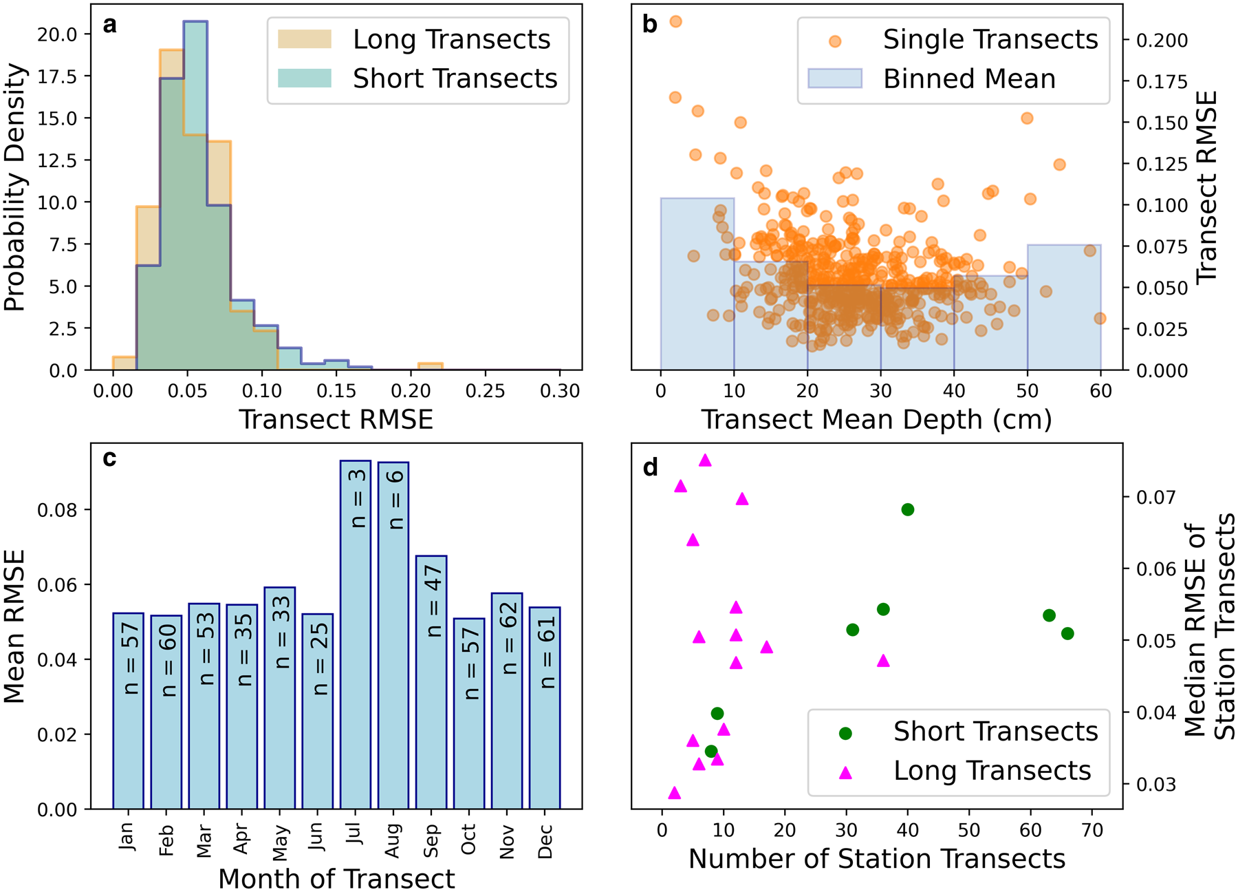
Fig. 5. (a) Histograms of the RMSE for long transects (1 km) and short transects (500 m) separately. (b) RMSE of the NP distribution against observed transects shown as a function of transect mean depth. (c) NP distribution RMSE as a function of month. ‘n’ indicates the number of transects contributing to the model from that month. (d) Median RMSE of all transects at a given station, shown as a function of the number of transects at that station. RMSE values are unitless as they represent the error in a probability distribution.
We first show that the NP model's skill is very similar when applied to both long and short NP transects (Fig. 5a). The mean RMSE for long and short transects is 0.053 and 0.057 respectively (a difference of 7%). This similarity is to be expected, with the difference likely reflecting the more incomplete sampling of the local snow depth distribution by a shorter transect. We also show that the skill of the NP distribution is relatively independent of the depth of the transect. The skill of the model is maximal for snow distributions with means in the range of 20–40 cm. Transects where the model exhibited lowest skill had very shallow depths (< 10 cm). In this category the model's skill is halved relative to the 20–40 cm range (which represents 69% of all transects). This mean-depth dependent skill reflects the relative representation of transects that contribute to the NP model: the model performs best when predicting transects similar to those on which it was trained (Fig. 3a).
The model's skill is relatively insensitive to the month of the year with the exception of July and August (Fig. 5c). In these two summer months its skill is diminished with the RMSE being on average 67% higher in these 2 months by comparison to the average of the other months. Again, this is ostensibly a reflection of the low contributions of these months to the total number of transects: July and August contribute three and six transects to the NP model respectively, whereas the other months on average each contribute 49 transects. Low skill in these months is also likely a reflection of the snow depths being lowest, which is also associated with low skill (see Fig. 5b).
We finally address the potential lack of independence between successive transects at the same station. Our LOOCV approach assumes that by not training the model with the transect being validated against, the validation transect is independent. But the potential exists that information about the validation transect enters the model through previous and subsequent transects at the same station that are included. If successive transects are strongly related, we would expect stations that contribute more transects to the model to have their transects perform better in the LOOCV exercise. Application of the non-parametric Spearman's rank test for correlation reveals no statistically significant relationship (p < 0.05) between the number of transects contributed by a station to the model and the mean or median RMSE of its transects in the LOOCV exercise (Fig. 5d). This supports the premise that LOOCV is an appropriate tool with which to evaluate the skill of the NP model.
Evaluation against MOSAiC measurements
We compare our regression and fitted curve (Figs 3a, b) against the snow surveys taken on the MOSAiC expedition using a magnaprobe (Figs 6, 7). To do this we select snow surveys of the ‘Northern Transect’ (Stroeve and others, Reference Stroeve2020b), which predominantly consisted of second-year ice.

Fig. 6. (a) Snow depth variability for a given mean depth was larger on the MOSAiC transects than on average for the NP stations. Regression for NP station data shown in red, MOSAiC transects in blue. (b) Because the depth variability is lower in the NP model, the probability distribution in standard deviation space is wider (as the standard deviations themselves are smaller).

Fig. 7. Winter evolution of the snow depth distribution on the MOSAiC Northern Transect (blue histograms, 5 cm bins). The modelled depth distribution described in this paper shown in red. Top right: plots of the 14 transects contributing to the MOSAiC evaluation exercise, with panel coordinates being the relative coordinates of the floe with the research vessel Polarstern at the origin orientated upwards).
We first note that the NP-based CV is lower than that observed on the MOSAiC transects (Fig. 6a). The effect of this is that the width of the modelled depth distribution is too high in standard deviation space (Fig. 6b), i.e. the NP model distribution is insufficiently ‘peaked’. Symptoms of this are underestimation of the two modal bins (relative to the MOSAiC data), and overestimation of the low tail probabilities. This extra width can be understood because the standard deviations are themselves smaller.
Despite this bias, the NP model generally provides a good fit to the individual MOSAiC transects (Fig. 7). The skewness parameter of the NP model (a = 2.54) is smaller than when a skew normal fit is applied to the MOSAiC transects (a = 6.4). This results in the modal depth bin often being overestimated by the NP model (Fig. 7). For clarity, the skewness parameter (a) of the skew normal distribution is different to the commonly calculated sample skewness (γ), although both quantities consistently have the same sign. We calculate and report the sample skewness for the NP data and all evaluation data in Supplementary Figure S2.
A corollary to this underestimation of skewness by the NP model is that that where the modal bin is overestimated by the model, the probability (or fractional coverage) of the depth bin is underestimated. This can be seen (e.g.) in the panel of Figure 7 corresponding to 30th January. The skewness parameter of data in this panel is 13.7, higher than that of the NP model. This results in the model's modal depth bin being one too high (20–25 vs 15–20 cm), and the probability of the modal bin being 3.5% too low. However, we recognise that the binning process involved in this comparison places a lower resolution limit on any comparison of modal values. As such, we also compare the modal value of the NP model with that of a skew normal curve fitted to each magnaprobe transect (Supplementary Fig. S3). We find that, similarly to Figure 7, the modal depth of the NP model is higher by comparison to the mode of the skew normal curve of best fit to the observations. This discrepancy grows over the winter from 2.7 cm at the start of October to 9.5 cm by the end of February. We stress that although a precise number can be determined for the difference in the mode of the NP model and the observationally derived curves, the curve-fitting process to the magnaprobe observations does not necessarily fully capture the underlying data, particularly with regards to the position of the modal value.
The fractional coverage of shallow snow is a key parameter for energy flux modelling, so is now given specific consideration. We find the NP model underestimates the coverage of thin snow (<10 cm) in early winter (end of October to mid December) with respect to MOSAiC observations. The observed coverage is 6.1%, and the NP model produces a coverage of 4.3%. After mid December the model begins to overestimate the thin snow coverage. On average it was observed to be 1.5%, and modelled to be 2.1%, an overestimate by 0.6 percentage points. With regards to heat fluxes, an overestimation of the thin snow coverage would lead to an overestimate of the heat flux from the ice to the atmosphere (and accompanying overestimation of sea-ice growth rate).
Evaluation against SHEBA measurements
We now evaluate our model using snow depth transect data from the Surface Heat Budget of the Arctic (SHEBA) expedition (Sturm and others, Reference Sturm, Holmgren and Perovich2002; Uttal and others, Reference Uttal2002). Snow transects were taken over a variety of ice types during the SHEBA expedition, and here we opt to compare our model to transects taken in the ‘Atlanta’ and ‘Tuktoyaktuk’ (henceforth ‘Tuk’) areas which were dominated by multi-year ice (for best comparison with the NP data). These areas were described using ice-class codes, and were indicated as 2–3 and 4 respectively. Class 2 indicates ‘Refrozen melt ponds’, 3 ‘Hummocky’ and 4 ‘Deformed’ (Sturm and others, Reference Sturm, Holmgren and Perovich2002). Snow depths were initially measured with a marked ski-pole, with a prototype magnaprobe being used later. While the NP model provides a good fit to the Atlanta transects, it is less appropriate for Tuk transects (where the RMSE is on average doubled compared to Atlanta).
Atlanta transects
We find the CV to be very similar between the SHEBA and NP transects (Fig. 8a). Removing transects from the high-melting month of July from the SHEBA data marginally improves this agreement, but not greatly relative to the uncertainty in the regressions. We note that no transects were taken in the Atlanta region in August.

Fig. 8. (a) Relationship between the mean snow depth and standard deviation of the snow depth on SHEBA ‘Atlanta’ transects (blue scatter). Linear regressions through the points are shown both including and excluding data points from July and August (blue solid and black dotted lines respectively). Linear regression from all NP transects shown by red line. (b) The snow depth distribution on the SHEBA ‘Atlanta’ transect excluding July and August (blue) and from NP stations (red). The SHEBA fit from all transects including July and August shown by black dotted line. (c) Time evolution of the error in this paper's model (blue scatter). RMSE is higher during July and August than in other months, which coincides with melted snow (depth in orange scatter).
Unlike the CV, the agreement of the snow depth distribution is clearly improved by removing July transects from the SHEBA distribution (Fig. 8b). We attribute this to strong alteration of the snow depth distribution by melt ponds in this month, which developed at the site in the second half of June (Webster and others, Reference Webster2015). Outside of this period the snow depth distribution is primarily dictated by wind redistribution, but within the period it is dictated by the production of liquid water at the surface of the snow, consequent runoff and potential melt pond formation.
The poor performance of our model in July and its association with intense snow melting is shown in Figure 8c. After strong melting (decreasing snow depth) in June, the snow depth distribution begins to diverge from the NP model during the transition from June to July, and increases throughout July.
Tuk transects
The NP model performs considerably less well when applied to Tuk transects (Fig. 9). Unlike Atlanta, the standard deviation of snow depth on Tuk transects is significantly underestimated by the NP regression. Furthermore, the skew parameter of the NP model (a = 2.54) is less than half that of a skew normal curve fitted to the Tuk transects (a = 6.27). The corresponding value for Atlanta is 2.9.
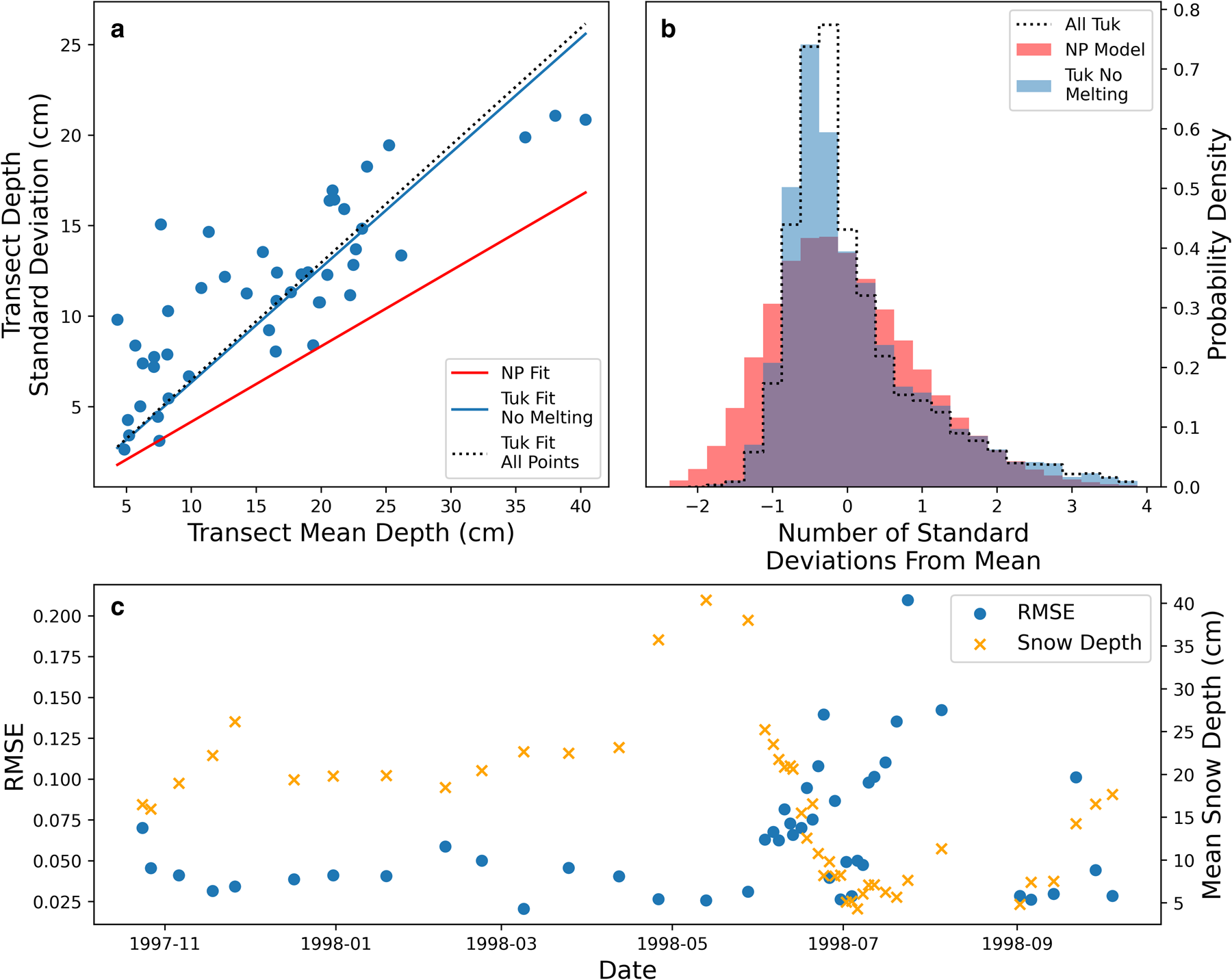
Fig. 9. (a) Relationship between the mean snow depth and standard deviation of the snow depth on SHEBA ‘Tuk’ transects (blue scatter). Linear regressions through the points are shown both including and excluding data points from July and August (blue solid and black dotted lines respectively). Linear regression from all NP transects shown by red line. (b) The snow depth distribution on the SHEBA ‘Tuk’ transect excluding July and August (blue) and from NP stations (red). The SHEBA fit from all transects including July and August shown by black dotted line. (c) Time evolution of the error in this paper's model (blue scatter). RMSE is significantly higher during July and August than in other months, which coincides with melted snow (depth in orange scatter).
It is striking that the mismatch in the skewness parameter for the Tuk transects is slightly smaller than the MOSAiC transects, but the model-observations mismatch is much larger. Furthermore it is notable that although the skewness of the Tuk transects is larger than the NP model, the NP model still does a good job of predicting the modal depth bin. We would expect the modal bin to correspond to snow depth that is too deep where the skewness is underestimated (see Fig. 7). These features are explained by the fact that a skew normal curve cannot be easily fitted to the Tuk transects in standard deviation space (Fig. 10).

Fig. 10. Distribution of relative depth anomalies for the three evaluation datasets used in this paper (red). Distributions were generated with a bin width of 0.5 standard deviations. Skew normal distributions are fitted to each and show variable agreement (black).
To illustrate, we display the transect data alongside the best possible skew normal fit (not involving the NP data) to the data. The agreement is good for the Atlanta and MOSAiC datasets, but noticeably less good for the Tuk data (Fig. 10). This indicates that unlike the MOSAiC northern transects and the SHEBA Atlanta transects, the SHEBA Tuk transects do not display a skew normal distribution of snow depths.
We attribute the deviation of the Tuk data from the skew normal distribution to the highly deformed nature of the ice relative to that seen at Atlanta and the MOSAiC northern transects, and at most of the NP stations. Firstly we point out that over strongly deformed ice the wind dynamics may cause snow to be distributed differently. Secondly we raise the fact that NP transects deviated around highly deformed ice such as that dominating the Tuk transects. There is a related sampling bias for the MOSAiC Northern transect, because the transect layout was chosen such that a snowmobile could drive around it.
Discussion
Negative snow depths
The use of a skew normal distribution results in a small fraction of negative snow depths. The total fraction is relatively constant at 0.1% in the 0–50 cm range of mean snow depths. Above this range, it transitions to a linear decline with increasing mean snow depth, dropping below 0.075% for snow depths larger than 200 cm (Supplementary Fig. S4).
Because the fraction of negative snow depths does not exceed 0.1%, we treat it as negligible in our analysis. However, if this distribution was implemented in a snow-conserving model it would be necessary to modify the low-tail of the distribution. This could be done by merging the distribution with an exponential curve at low values, or by truncating it at zero and redistributing the coverage so that the area under the probability distribution is unity. In the redistribution case, it would be possible to either scale the whole curve by a small amount, or instead preferentially add the ‘lost’ coverage to the low-end of the distribution. We stress however that the effect of this would be extremely small (and not noticeable in the analysis of this paper), and so is only necessary for applications where snow must be precisely conserved. For completeness we point out that when a log-normal distribution is fitted to the data in Figure 3a (instead of a skew normal), the fraction of negative snow depths is a similar function of the mean depth as in the skew normal case, but ~100 times smaller in magnitude.
Potential for application to first year ice
No multi-station data similar to the NP transects exist for first year ice (FYI). This is in part because FYI cannot be drifted on for long before experiencing a melt season, but also because FYI is thinner and more liable to break up, making crewed research installations difficult to establish. Because of these difficulties, it is natural to wonder whether the NP snow depth distribution can be applied to FYI and with what uncertainty. To investigate this we apply the NP model to FYI snow depth transects taken on the AMSR-Ice03, AMSR-Ice06 (Sturm and others, Reference Sturm2006) and MOSAiC field campaigns (Krumpen and others, Reference Krumpen2020). Several of these transects were performed in Elson Lagoon (EL in Fig. 11), which consists of level ice. This contrasts with the more deformed ice on the nearby Beaufort sea measured during AMSR-Ice03 (BS in Fig. 11). During AMSR-Ice06 a level-ice section in the Chukchi Sea was also surveyed (CS in Fig. 11). Finally, during the MOSAiC expedition, successive transects were taken on a refrozen lead (nicknamed the ‘runway’, described in Stroeve and others (Reference Stroeve2020b)), which provides some information about the thin-snow regime on FYI (Figs 11g, h, i). For the eight transects described above we calculate the RMSE of the NP model when applied based on the mean value, calculated with 5 cm bins. We also fit a skew normal curve to the transect data and investigate the skewness parameter (a) to shed light on the mismatch between the NP model and the observations.

Fig. 11. Comparison of the NP model with data from FYI transects taken during the AMSR-Ice03, AMSR-Ice06 and MOSAiC field campaigns. Panel (a) shows the ratio of snow depth standard deviation to transect mean depths (the CV) for the FYI transects (large markers) as well as for the NP transects (grey dots). All other panels show the snow depth distribution produced by the NP model (red) against the transects (blue), with 5 cm wide depth bins for comparative purposes. Panels represent (in order b–i) Elson Lagoon (EL) and level ice on the Chukchi Sea (b and c), two transects on Elson Lagoon one week apart (d and e), a transect on FYI of the Beaufort sea near Elson Lagoon (f). Bottom row (g–i) displays snow transects taken on a refrozen lead during the MOSAiC expedition.
We first observe that all eight FYI transects have CV values roughly consistent with that observed in the NP stations (Fig. 11a), particularly those from AMSR-Ice06. The average difference between the FYI CV values and that of the NP model is 0.74 (a unitless quantity), or ~17% of the CV of the NP model. We display the CV values for all FYI data in Supplementary Figure S5. We also note that the skewness parameter of the AMSR-Ice06 data (a = 1.6 and 2.2) is close to the skewness parameter of the NP model (a = 2.54). These characteristics lead to the NP model performing better on the AMSR-Ice06 data than the AMSR-Ice03 data. The AMSR-Ice06 survey on Elson Lagoon has the lowest RMSE of all eight FYI transects (0.012) when compared to the NP model – this is related to it having the most closely matching skewness parameter to the NP model.
While all three AMSR-Ice03 transects have very similar mean snow depths to each other (~ 30 cm), the CV is lower than the NP station transects for the Elson Lagoon transects, but higher for the Beaufort Sea (Fig. 11a). That is to say, the snow over the deformed FYI in the Beaufort Sea exhibited considerably more variability than that over the level ice in Elson Lagoon during AMSR-Ice03. In addition to being more variable, the Beaufort Sea transect showed a much higher skewness parameter (a = 5.14) than those on Elson Lagoon (a = 1.02 and 0.844). The transect over deformed ice exhibits the lowest RMSE value of the AMSR-Ice03 transects by some margin.
We attribute the low-skewness (symmetry) of the 2003 Elson Lagoon data to a lack of ice topography around which to build up a ‘long tail’ of drifted, thick snow. Conversely, the highly deformed ice of the Beaufort Sea produces a noticeable long tail of thick snow, such that the probability of finding snow deeper than 55 cm is underestimated by the NP model (Fig. 11f). However, it is striking that the AMSR-Ice06 transects at Elson Lagoon are more weakly governed by this: while the skewness parameters are still lower than for the NP transects, there is a smaller difference. It is possible that this variability is produced by the cumulative effect of wind redistribution, and particularly strong wind events. Investigating the role of strong-wind events on the CV and skewness of the snow depth distribution may form the basis for future work.
We now turn to the thin snow cover of the three MOSAiC ‘runway’ transects (Figs 11g, h, i). We first point out that a skew normal curve cannot be easily fitted to these data (Supplementary Fig. S6; similar to the situation with the SHEBA ‘Tuk’ transects above). This indicates that the NP model will not be a good fit, even before it is applied. Because of this feature, the skewness parameter values listed in the panels of Figure 11 should not be assumed to properly capture the underlying transect data. When the NP model is applied and compared, it exhibits a high RMSE relative to the other FYI transects. As well as being related to the poor approximation with a skew normal curve, this performance is also linked to the three ‘runway’ transects having the highest error in the CV (Fig. 11a) by comparison to the NP transects. One key physical difference between the runway transects and the other FYI surveys is the low average snow depth. However, other contextual differences exist: for example the transects were performed in a colder region (near the pole), and at a colder time of year (January/February). This may result in a more weakly bonded snowpack at the time of measurement, susceptible to more wind-redistribution and resulting in a higher CV (by comparison to the AMSR-Ice transects).
Because of the differences in the age of the snow (and the ice topography over level ice), there is no a priori reason that the NP model for the snow depth distribution derived in this paper should be applicable to FYI, and indeed our model works relatively poorly when simulating the ‘symmetrical’ snow depth distributions at Elson Lagoon in 2003, and the thin snow on the MOSAiC runway.
However, in the instance where the ice was deformed (Fig. 11f) the model performs relatively well. Perhaps counterintuitively given the 2003 results, the NP model also performed well in 2006 over both level ice transects. The RMSE of the NP model when applied to the Beaufort Sea transect was 0.016, which is in fact lower than the corresponding values for the MOSAiC northern transects (Fig. 7), which ranged from 0.019 to 0.031. By this metric the performance of the model over FYI in 2006 was also better (lower RMSE, 0.012) and comparable (similar RMSE, 0.022).
In summary, we have shown that the NP model is capable of performing well over deformed FYI, and even over level ice in the case of 2006 (where ‘well’ is defined with reference to its performance over second-year ice at MOSAiC). But despite this capability, it also clearly performs poorly in the case of thin snow (at MOSAiC runway, where we observed that the measurements could not be well-represented by any skew normal distribution), and also in the case of highly symmetrical (low-skew) snow distributions over FYI (Elson Lagoon in 2003).
Application to point-measurements of snow depth
There are several drifting, autonomous platforms in existence that record the snow depth at a single point, such as snow buoys and ice mass balance buoys (Nicolaus and others, Reference Nicolaus2021). If the buoy is deployed at random, it is most likely to sample the modal snow depth. In reality these instruments are often not deployed at random, and a conscious choice is made to sample what is perceived to be the modal depth. However, for applications such as laser and radar altimetry retrievals of sea-ice thickness, the mean snow depth is the quantity required for characterising the floe's hydrostatic equilibrium (e.g. Mallett and others, Reference Mallett2021). We now present a simple method of relating these point measurements to the mean snow depth of the surrounding area.
If the mean snow depth ($\overline {D}$ ) is related linearly to the standard deviation (σD, Fig. 3a, Eqn (1)) by the CV, and we observe the modal snow depth to be X SDs below the mean (Fig. 3b), then we can relate the modal depth to the mean depth as follows:


Using the NP data from Figure 3 we now calculate that X = 0.35. The CV was found earlier (Eqn (1)) to be 0.417. We therefore calculate that the mean snow depth is 17% larger than the modal depth. Where singular drifting instruments are assumed to retrieve the modal snow depth in their environment, we recommend this correction for estimation of the mean.
Length scales
The NP station transects were performed over distances of 500–1000 m, and this characterises the length scale on which our distribution is relevant. If the same transects were theoretically performed over just a few centimetres, the CV (Fig. 3a) would be lower, and the distribution about the mean would likely be different. The distribution would be sensitive to the small-scale roughness of the snow surface, rather than larger-scale features like sastrugi and snow drifts around ice topography. If the transects were performed (again, theoretically) over thousands of kilometres then the snow distribution would again be different, and more representative of synoptic variability in snowfall and ice type. As such we stress that the distribution of snow depths has been characterised at the sub-kilometre length scale (on the order of hundreds of metres).
We also investigate the sensitivity of our analysis to the spatial sampling interval of the transects, which was 10 m for the NP stations. In particular, we consider the possibility that adjacent (and near-adjacent) snow depth measurements on a given transect may be correlated (Moon and others, Reference Moon2019), and the impact that this might have on our main results. To do this we perform an autocorrelation analysis for each of the 499 transects, testing the correlation of a spatially lagged series against the original set of measurements. We find that for a lag of one measurement (10 m), 26% of transects show a statistically significant autocorrelation (p < 0.05). To put this another way, we detect that adjacent points are correlated in 26% of transects. This fraction drops by roughly half at a lag of 2 measurements (20 m, 12%), and half again for a lag of 3 (30 m, 7%; Fig. 12a). We performed our test for correlation at the 5% level (i.e. significance at p < 0.05), and as such would predict one in 20 transects to exhibit a correlation even in the case where all snow depth measurements were sampled randomly from a normal distribution. As such, we see the fraction of statistically significant transects tend to this level at higher lag values (Fig. 12a). We also analyse the strength of positive autocorrelations where they are statistically significant. The typical strength (r value) of these statistically significant correlations is broadly similar (0.364, 0.315 and 0.31 respectively for lag = 1, 2 and 3; Fig. 12b).
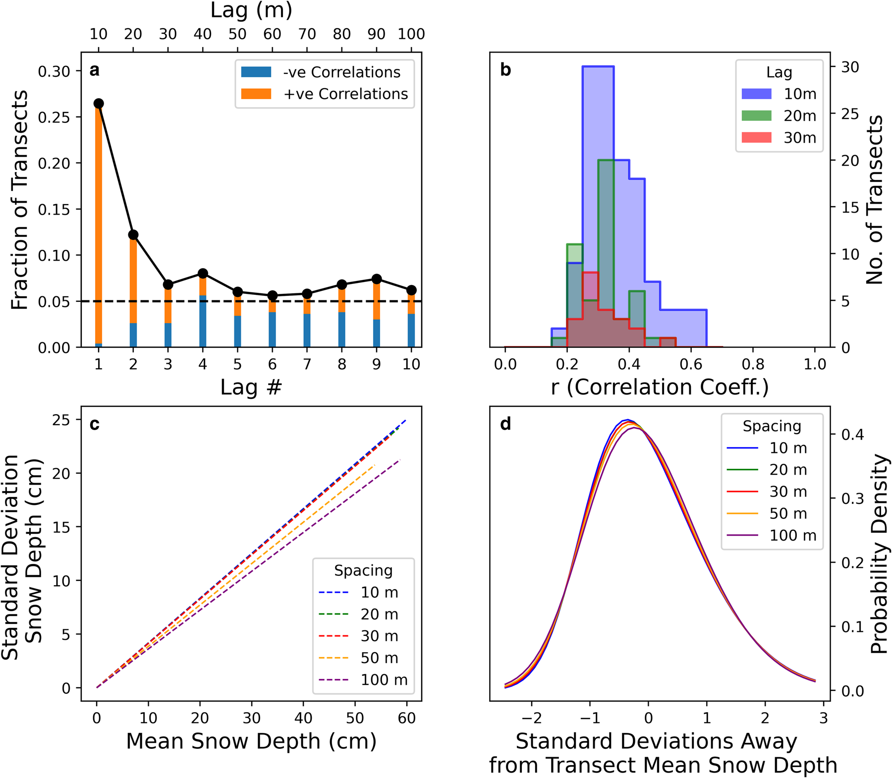
Fig. 12. (a) Fraction of transects with a statistically significant autocorrelation at various lags. A total of 26% of transects exhibit correlated adjacent measurements at lag = 1. (b) The distribution of Pearson r correlation coefficients for various lags, where correlations are statistically significant. The mean strength of the statistically significant correlations decreases slowly as the lag increases. (c) Impact of undersampling the transect by taking every second, third, fifth and tenth measurement on CV, and (d) the probability density distribution in standard deviation space. The impact of this sampling is small for the double-spacing and triple-spacing, indicating that the correlation of adjacent points in 28% of transects has a negligible impact on the main results in this paper.
The effect of adjacent points being correlated on our main analysis can be obviated by only analysing every other transect measurement. To remove the effect of autocorrelation for a lag of two samples, we can perform our analysis again but only consider every third measurement, etc. The results of this exercise on the main results are displayed in Figures 12c, d (cf. Figs 3a, b). The CV (Fig. 12c) is essentially unchanged by only analysing every second or third measurement from the transects, and this is also true for the calculated skew normal distribution (Fig. 12d). To stretch this approach, we also display the results of taking every fifth and tenth sample from transects. When comparing a 10 m sampling interval to a 100 m sampling interval, the CV decreases from 0.416 to 0.361, and the skewness parameter decreases from 2.54 to 1.84. Extrapolating from this trend, magnaprobe samples used in the validation datasets which have a very low sampling interval of 1 m may therefore have a high-skew and high coefficient of variation bias relative to transects from NP stations. However, the corresponding analysis for these datasets is significantly more complex as, unlike the NP transects, the samples were generally neither regularly spaced nor taken along a straight line.
For completeness we also investigate a common statistic for correlation between adjacent measurements: the correlation length (Supplementary Fig. S7). This is calculated for a transect by, as above, calculating the correlation of lagged transects with the original transect at increasing lags. The correlation length is then defined as the lag at which the correlation drops to a value of 1/e. Because only a minority (28%) of transects have statistically significant correlations for adjacent points (Lag = 1 sample, 10 m), the correlation lengths for the transects are generally below 10 m. Because of the coarse spatial resolution of the measurements, we must interpolate to get the correlation length, and this was done linearly. When calculating in this way, we find the modal correlation length of the transects to be 6.8 m (Supplementary Fig. S7b), although this would be highly sensitive to the interpolation method. In total, 9.4% of transects had a correlation length of 10 m or greater.
Relevance in a changing Arctic Ocean and other limitations
The potential for application of the NP model to FYI was discussed above, and it was found that while the NP model was capable of performing well over FYI, it performed poorly when simulating the distribution of thin snow, and overestimated the skew in some cases. Here we point out that the Arctic Ocean is becoming increasingly dominated by FYI, so arguably the relevance of this multi-year ice trained model is in slow decline.
There may also be spatial limitations on applicability. The NP drifting stations generally operated in the Central Arctic Ocean (Fig. 1) rather than in the marginal regions such as the Kara, Beaufort and Barents seas (Warren and others, Reference Warren1999). However, these areas are generally dominated by FYI, so this geographic constraint is less strict that the ice-type one described above.
The average age of multi-year ice is in decline, with the coverage of ice aged 5 years or more shrinking from 28 to 1.9% between 1984 and 2018 (Stroeve and Notz, Reference Stroeve and Notz2018). The mean thickness of sea ice is also in decline (Kwok, Reference Kwok2018). Because we produce our statistical model using drifting station data from 1955 to 1991, it likely reflects snow conditions on ice older and thicker than that which currently exists in the Arctic. We note however that our model does still display good skill with respect to the MOSAiC transects, which were generally performed on ice that had only experienced one melt season.
Summary
In this paper we have developed a generic snow depth distribution for multi-year ice that can be fully characterised by the mean snow depth. This allows it to be superimposed onto estimates of mean snow depth from satellites and models for the purposes of flux modelling and altimetry studies.
We performed a cross-validation exercise and found the model's skill to be highest in winter, and lowest during the summer months of intense melt and sparse measurements. We then evaluated the distribution against snow depth transects from the MOSAiC, SHEBA and AMSR-Ice field campaigns. These analyses revealed that the model generally overestimated the variability in snow depths for the MOSAiC campaign, but the fit parameters were otherwise broadly appropriate. On the smoother multiyear ice of the SHEBA campaign the model performed well, but the model performed poorly on transects executed over highly deformed ice. This was related to the fact that the snow depth distribution in this area was not well approximated by the skewed normal distribution used in the NP model. Application of the distribution to eight transects conducted over FYI shows that while the NP model was capable of performing well (over deformed FYI and in two cases over level ice), it performed poorly when simulating thin snow on a refrozen lead in the Central Arctic, and also when simulating a highly symmetrical snow distribution over level ice.
Supplementary material
The supplementary material for this article can be found at https://doi.org/10.1017/jog.2022.18.
Code and data availability
All code and data required to reproduce this analysis can be downloaded from: www.github.com/robbiemallett/sub_km.
Acknowledgements
This work was funded primarily by the London Natural Environment Research Council (NERC) Doctoral Training Partnership (DTP) grant (NE/L002485/1). JCS acknowledges support from the Canada 150 Chair Program and NASA grants NNX16AJ92G, 80NSSC20K1121 and 19-ICESAT2-19-0088; ‘Sunlight under sea ice’. MT acknowledges support from the European Space Agency ‘Polarice’ grant ESA/AO/1-9132/17/NL/MP, NERC grant NE/S002510/1, NERC ‘PRE-MELT’ NE/T000546/1 project and from the ESA ‘EXPRO + Snow’ (ESA AO/1-10061/19/I-EF) project. VN was supported by JCS, in part thanks to the Canada 150 Chair Program. RW was supported by NERC grant NE/S002510/1. PI acknowledges funding from the Research Council of Norway (RCN287871, SIDRiFT) and the US National Science Foundation (NSF) (NSF1820927, MiSNOW). MO acknowledges funding from the NSF (OPP1735862). MJ acknowledges funding from the NSF (NSF1820927, MiSNOW). JL acknowledges support from the Centre for Integrated Remote Sensing and Forecasting for Arctic Operations (CIRFA) project through the Research Council of Norway (RCN) under Grant RCN237906. We wish to thank the reviewers and editor for their guidance and suggestions during the review process.
Author contributions
RM developed the NP model in consultation with JS, MT, RW and VN. JL, PI, MO, MJ and DP were involved in collecting, providing and advising on the evaluation data. All authors contributed to and provided feedback on the manuscript.


 Open access