


1. Introduction
Subsurface heat conduction, the heat transport between the subsurface snow/ice layer and the surface, is an important component of the surface energy balance (SEB) between the cryosphere and the atmosphere. Subsurface heat conduction may even act as an important energy source for the SEB due to its compensating effect during periods of low solar radiation (Van den Broeke and others, Reference Van den Broeke, Reijmer, Van As, Van de Wal and Oerlemans2005a; Ding and others, Reference Ding, Anubha, Heil and Yang2019). In addition, subsurface heat conduction, by propagating temperature fluctuations downward, is the key control of the upper thermal boundary of the entire Antarctica and Greenland ice sheet, and may ultimately affect glacier dynamics (Creyts and others, Reference Creyts2014; Ding and others, Reference Ding2021). However, due to its small magnitude compared with other energy components, its contribution has not been addressed in early studies (Arnold and others, Reference Arnold, Willis, Sharp, Richards and Lawson1996; Matthias and others, Reference Matthias, Saurer and Vogt2001), possibly resulting in a significant error for the estimations of SEB in the polar regions (Jakobs and others, Reference Jakobs, Reijmer, Munneke, König-Langlo and Van den Broeke2018). Particularly for mountain glaciers, the melting and mass loss of snow/ice surfaces is overestimated when subsurface heat conduction is ignored (Pellicciotti and others, Reference Pellicciotti2008; Wheler and Flowers, Reference Wheler and Flowers2011). Although subsurface heat conduction is often neglected in areas without melt (e.g. Antarctica inland regions), it might still influence turbulent heat exchange and even sublimation (Ding and others, Reference Ding2020). A study by Van den Broeke and others (Reference Van den Broeke, Reijmer, Van As, Van de Wal and Oerlemans2005a) in Dronning Maud Land in 1998–2001 showed that the surface heat conduction could contribute up to 30% of the energy transport toward the surface in April and remove up to 50% of the energy from the surface in November and December.
Several studies have implicitly considered snow and ice subsurface heat conduction in the SEB (Carroll, Reference Carroll1982; Van As and others, Reference Van As, Van den Broeke, Reijmer and Van de Wal2005; Van den Broeke and others, Reference Van den Broeke, Reijmer, Van As, Van de Wal and Oerlemans2005a). However, direct measurements of subsurface heat conduction in the snow layer are not simple as they disturb the snow structure (Van As and others, Reference Van As, Van den Broeke, Reijmer and Van de Wal2005) and there are few in situ observations for reference. Validating the applicability of the snow/ice heat conduction parameterization scheme under different climatic backgrounds and topography has also been limited. For simplicity, most of the conduction terms have been computed from empirical parameterizations (Yen, Reference Yen1981; Greuell and Konzelmann, Reference Greuell and Konzelmann1994; Sturm and others, Reference Sturm, Holmgren, König and Morris1997; Calonne and others, Reference Calonne2011), although some studies have characterized the Antarctica subsurface heat conduction in both inland and coastal regions (e.g. South Pole, Dome C and Halley stations) using energy-balance residuals or thermal parameterization scheme methods (Carroll, Reference Carroll1982; Van As and others, Reference Van As, Van den Broeke, Reijmer and Van de Wal2005; King and others, Reference King, Argentini and Anderson2006; Town and Walden, Reference Town and Walden2009). However, to date, only a few complete spatial and annual studies on subsurface heat conduction have been carried out and discussed (Van den Broeke and others, Reference Van den Broeke, Reijmer, Van As, Van de Wal and Oerlemans2005a; Van den Broeke and others, Reference Van den Broeke, Reijmer, Van As and Boot2006).
To improve our understanding of subsurface heat transfer and further enhance numerical forecast models over Antarctica, especially in the inland katabatic and plateau zones, it is necessary to determine the subsurface heat conduction features under different climatologies. In this paper, we quantify the characteristics of subsurface heat conduction at the LGB69, Eagle and Dome A stations (Fig. 1), which are situated in three different climatological zones along the CHINARE (Chinese National Antarctic Research Expedition) traverse route. We also compare our results with other Antarctic regions and analyze the factors that may affect the vertical heat conduction. Section 2 of this paper introduces the three study areas and the calculation of subsurface heat conduction. Meteorological conditions and snow layer (temperature and density) and subsurface heat conduction characteristics are systematically described in section 3. Section 4 provides a discussion of the comparison with other Antarctic sites. Forcing from the atmosphere and the uncertainty evaluation are also included in this section. Section 5 presents the conclusions.

Fig. 1. (Upper) Topography (shaded) and location of automatic weather stations. (Bottom) The elevation variation along the CHINARE traverse.
2. Data and methods
2.1. Study regions
The CHINARE traverse route starts from Zhongshan station (76.4°E, 69.4°S) and ends at Dome A, covering a distance of ~1248 km (Ding and others, Reference Ding2015) along ~77°E longitude. Controlled by the large-scale slope of the ice sheet and the gravitational force of cold air masses, the distribution of prevailing katabatic winds shows considerable spatial variability. The katabatic winds influence the surface mass balance and can form ‘glazed surface’ on leeward slopes of the ice sheet (Scambos and others, Reference Scambos2012; Ding and others, Reference Ding2015). The traverse route includes five different surface morphological zones (Ding and others, Reference Ding2011): steeply sloping coastal zones, gradually rising zones, extremely flat zones, ice-divide zones and dome summits. The different zones have different climatological and surface mass-balance characteristics, making the traverse route ideal for comparative studies of the SEB.
In this study, we analyze the subsurface temperature, heat conduction features and their relation with the meteorological conditions at three automatic weather stations (AWSs) along the CHINARE traverse: These are LGB69, Eagle and Dome A stations: the locations of these sites are shown in Figure 1. As the distance to the coast and the elevation increase, the surroundings of the three stations exhibit significant morphological differences and can represent typical Antarctic coast, inland and dome environments.
The LGB69 station (deployed in 2002) is located in Princess Elizabeth Land, on the eastern side of the Lambert Glacier basin (LGB), at 77.1°E, 70.8°S, 1854 m a.s.l. This station is the closest of the three to the coast. It has an average slope of 11 m km–1, and is downstream of the region with the steepest slope on the ice sheet. This station can also be affected by cyclone invasions, resulting in an Antarctic maritime climate.
The Eagle station (deployed in 2005) lies at 77.0°E, 76.4°S, 2852 m a.s.l. This is inland between the highest plateau region and the coastal zone, with an estimated large-scale surface slope of 4.3 m km–1 (Ding and others, Reference Ding, Anubha, Heil and Yang2019). This region is under the influence of a stable katabatic wind, and is called the inland katabatic wind region.
The Dome A station (also deployed in 2005) is situated at 77.4°E, 80.4°S, 4093 m a.s.l. This is at the end of the traverse route, 1248 km inland from the coast, at the summit of the East Antarctic ice sheet. Due to its low surface slope (~2.6 m km–1) and high altitude, it is free of the influence of the katabatic wind (Ding and others, Reference Ding2011).
2.2. Sensor specifications and data processing
The same sensors were fitted on the three AWSs. Naturally ventilated air temperature, relative humidity and wind speed were recorded at an initial height of 2 m above the snow surface. In addition, snow temperature probes were installed at initial depths of 0.1, 1 and 3 m below the surface. The data sampling interval for all sensors was 10 min and stored as 1 h average values. Detailed sensor specifications can be found in Ma and others (Reference Ma, Bian, Xiao, Allison and Dou2010).
To reduce the effect from disturbance of the snow layer during installation, the selected observation period used in this study was from 2005 to 2006 for LGB69 and from 2008 to 2011 for Dome A and Eagle. Because the anemometer was often frozen during wintertime, a wind data gap always occurred each year. Ding and others (Reference Ding2020) suggested that the 10 m wind speed of ERA5 reanalysis (Hersbach and others, Reference Hersbach2018) and observed 2 m measured wind speed compared well, with a yearly average bias and root mean square error of −0.4 and 1.5 m s–1, respectively. Therefore, we filled the AWS wind speed data gaps using ERA5 reanalysis datasets, linearly interpolating from the nearest ERA5 grid points. Vertical snow density profiles were measured at LGB69 only in 2005, and at EAGLE and Dome A only in 2008. These were supplemented with nearby CHINARE snow pit measurement data at times closest to our analysis periods (Ding and others, Reference Ding2021). Small changes in the snow temperature probe depths with snow accumulation were not considered.
2.3. Calculation of the subsurface heat conduction
Penetration of the solar radiation into the snow layer is limited and decreases exponentially with depth. Because of a lack of radiation observations, this penetration of the solar radiation was not specified in this paper. With this assumption, the subsurface heat conduction G c was calculated using the effective thermal conductivity K s from the hourly snow temperature data (Sun and others, Reference Sun2018; Liu and others, Reference Liu2021).

where ∂T/∂z is the snow temperature gradient. All terms are defined positive when directed toward the surface. K s was determined as follows:

here, k, C p and ρ are the apparent thermal diffusivity (ATD), specific heat capacity and density of the snow, respectively. To achieve a high temporal resolution for thermal characteristics, an iterative optimization method for the ATD was applied depending on snow temperature, which had a better performance than temperature phase-change and density-based parameterizations for temperature modeling (Oldroyd and others, Reference Oldroyd, Higgins, Huwald, Selker and Parlange2013; Yang, Reference Yang2019). In the algorithm, an iterated ATD k i was substituted into the 1-D thermal diffusion equation to simulate the corresponding snow temperature T mod, n in the next temporal step,

where t is time, and the errors between the modeled and the measured snow temperature (T mod, n and T mea, n) for the period were obtained. Finally, the ATD of each time window with the minimum overall error ${\rm Min}\left({\mathop \sum \limits_{{\rm days}} {( {T_{{\rm mea}}-T_{{\rm mod}}} ) }^2} \right)$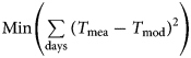 that best represented the snow physical processes was selected. To make the method robust, the search range of the ATD was chosen from 1 × 10⁻⁹ to 1 × 10⁻⁵m2 s–1 following Yang (Reference Yang2019), and the iteration step and time windows were set as 1 × 10⁻⁹m2 s–1 and 90 d, respectively.
3. Results
3.1. Meteorological conditions
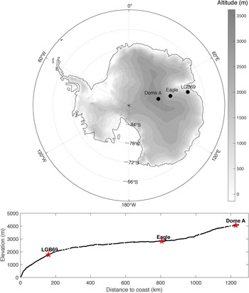
Using the AWS measurements and ERA5 reanalysis datasets, the daily mean variations in 2 m air temperature, relative humidity, air pressure and wind speed are shown in Figure 2. Data from the three stations exhibited large diversity in that the daily mean air temperature records decreased from coastal to inland plateau areas (Fig. 2) and reached a low of −77.2°C at Dome A during wintertime (Table 1). Similar to Van den Broeke and others (Reference Van den Broeke, Van As, Reijmer and Van de Wal2005b), the temperature disparities at different stations could not be simply explained when only the temperature lapse rate in Antarctica was considered (Yamada and others, Reference Yamada1974). Even in winter, LGB69 showed a warming bias ~5°C compared to the lapse rate corrected temperature (1.1–1.2°C 100 m–1) at the Eagle station. A large-scale pressure gradient force results in response to the negative net radiation and the ice-sheet topography, leading to a sustained, strong katabatic wind and a dry adiabatic effect on the air temperature at the stations (Van den Broeke and others, Reference Van den Broeke, Van Lipzig and Van Meijgaard2002). The lapse rate decreased to 0.87°C 100 m–1 from Eagle to Dome A (Ding and others, Reference Ding2015) due to its flat slope.

Fig. 2. Daily mean value of (a) 2 m air temperature; (b) relative humidity and (c) wind speed during 2005–2007 (LGB69) and 2008–2012 (Dome A and Eagle).
Table 1. Annual mean of air temperature, relative humidity, wind speed (2 m), snow temperature and density at LGB69, Eagle and Dome A

Because there is no winter shortwave radiation at these high latitudes, the air temperatures did not change much from month to month during winter. Allison and others (Reference Allison, Wendler and Radok1993) showed that inland stations did not have distinctive minima during winter which were called the ‘coreless’ winter. This phenomenon has long been known in Antarctica (e.g. Meinardus, Reference Meinardus, Köppen and Geiger1938). A coreless-ness parameter is calculated as the amplitude ratio of the second to the first harmonic of the annual temperature wave. A typically ‘coreless’ winter was considered to have happened if the coreless-ness was larger than 0.25. At our sites, the coreless-ness showed an increased distribution from coastal to inland areas, with an inland annual mean value of 0.40 and a coastal annual mean value of 0.34, which both indicated ‘coreless’ winter characteristics. On a daily scale, however, the air temperature showed a strong variability and a larger variation in coastal regions. The air temperature may have been affected by the fluctuation in the Antarctic atmospheric system, which could be the result of frequent approaches of cyclones to the Antarctic continent from lower latitudes (Ding and others, Reference Ding, Anubha, Heil and Yang2019).
In addition, the meridional temperature gradient of air temperature in winter was greater than that in summer, as was the inter-annual variability. This variability could cause greater air temperature fluctuations, especially when the warm air mass invades southward during winter (Ding and others, Reference Ding, Anubha, Heil and Yang2019). Furthermore, at all sites, the temperature gradient between the snow surface and the lower atmosphere reached a maximum value in winter, when the air temperature gradient reversed and led to negative sensible heat fluxes.
Determined by the combined effects of the katabatic wind and the Coriolis force, the persistent wind direction is west of the fall-line slope. The daily average wind speed peaked, with a value >20 m s–1, at the largest slope area (LGB69). Both Eagle and LGB69 stations had significant seasonal variability in wind speed. But Dome A station, which is on the East Antarctic ice-sheet summit had a relatively low wind speed and little seasonal variability. The katabatic winds vertically mix the air and resulted in 5–10°C increase in the air temperature near the surface. However, this process is not active when the katabatic forcing becomes weak in summer (Van den Broeke and others, Reference Van den Broeke, Van As, Reijmer and Van de Wal2005b).
The relative humidity decreased inland (Table 1). The seasonal cycle of relative humidity had little change at LGB69 and a more marked change at the other two stations, similar to the seasonal air temperature cycle. During the entire year, the daily mean relative humidity at LGB69 typically varied between 60 and 80%, whereas at Dome A and Eagle, it varied between 30 and 70%.
3.2. Snow density
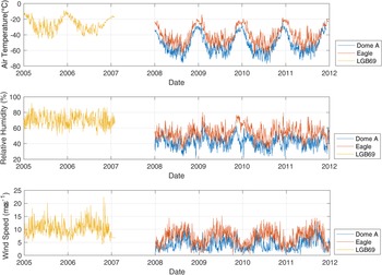
The snow density depends on many factors, including surface wind speed, air temperature, the ice-water ratio of the snow layer and purity (Yen, Reference Yen1981). The CHINARE traverse route has varying topography, which results in different levels of wind-driven effects and snow accumulation rates in different sections. According to the results of Ding and others (Reference Ding2015), the average snow accumulation rates at LGB69, Eagle and Dome A were 155.2, 64.6 and 28.0 kg m–2 a–1, respectively. Ding and others (Reference Ding2011) indicated that the snow density decreases from the coast along the traverse route as the wind speed decreases. This was in good agreement with the snow densities shown in Figure 3, with the density of the top snow layer decreasing from 482.6 kg m–3 under the influence of the katabatic wind to 266.7 kg m–3 in the Dome A regions. The vertical density distribution for the Dome A and Eagle stations generally showed a zigzagging increase with depth and relatively high std dev. of up to 47.4 kg m–3. These fluctuations might result from the intense seasonal variations in solar radiation. In the summertime, more solar energy is transmitted into the underlying firn than in wintertime, resulting in the large temperature gradient between the solar-heated layer and colder firn at depth. This process could drive extensive depth-hoar formation, resulting in a sharp increase in the density profiles (Scambos and others, Reference Scambos2012). However, similar density discontinuities did not occur at station LGB69, where the moisture and heat properties were more stable. At LGB69, the vertical average density and maximum difference in density were only 509.3 and 88.1 kg m–3, respectively. In addition, the density at the Dome A station had a significant overall increase below a depth of 1.8 m, which might result from long-term densification and metamorphism.

Fig. 3. The firn depth-density profile at LGB69 (measured in 2005), Eagle and Dome A (measured in 2008).
3.3. Snow temperature
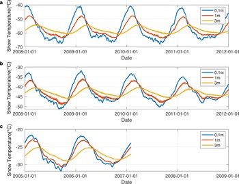
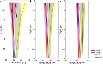
Figure 4 shows that measured snow temperatures at all depths peaked between January and March. As with air temperature, the largest daily snow temperature wave occurred during cold periods when the stable and strong katabatic wind exerted control, suggesting an influence from the Antarctic atmospheric system on the subsurface snow layer, even in periods lacking shortwave radiation. Otherwise, although the snow temperature revealed obvious seasonal variations, the mean diurnal variations did not exhibit significant fluctuations (not shown in detail here). Vertically, snow temperatures fluctuated less from the deep to the upper layers, and the amplitudes at a depth of 3 m were reduced to ~1/4 to 1/3 of the amplitudes of the upper layers. The snow temperature profiles always monotonously changed with depth and showed a very distinct seasonal differences (Fig. 5). The vertical temperature gradient during winter (June, July, August) was opposite to that in summer (December, January, February), and the inter-annual std dev. was less in winter than other seasons. At all stations, snow temperature below the 2 m depth was warmest in autumn (March, April, May) and coldest in spring (September, October, November), indicating a snow temperature phase lag effect.

Fig. 4. Daily mean value of snow temperature at the depth of 0.1, 1 and 3 m.

Fig. 5. The average snow temperature profile in Dome A, Eagle and LGB69 during four seasons (the shaded boundaries are the ±1 std dev.).
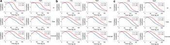
This large temperature lag results from the low thermal conductivity of snow (Chen and others, Reference Chen, Zhang, Xiao, Bian and Zhang2010). The uppermost snow layer could react rapidly to atmospheric forcing, particularly during periods of strong solar radiation (Vihma and others, Reference Vihma, Mattila, Pirazzini and Johansson2011). To investigate whether the snow thermal properties are different at the three AWS sites, and at different depths in the snow pack, we analyzed the lag time for a snow temperature signal at a depth of 0.1 m to reach depths of 1 and 3 m. Further, to also determine any role of shortwave radiation in heat transfer within the snow, we also analyzed this lag time under different cloud cover conditions (cloud coverage from 0 to 3/8 was considered ‘clear’; cloud coverage from 6/8 to 1 was considered ‘overcast’), and for daytime and nighttime (daytime and nighttime were defined on the basis of the presence and absence of shortwave radiation) (Fig. 6). The results showed sensitivity in the response times. Almost all of the stations in the four situations (clear/overcast and day/night) monotonically increased and then decreased with different slopes. All the maximum correlation coefficients were nearly 1.

Fig. 6. The correlation coefficient-time lag between 0.1 m and lowest two-layer (1 and 3 m) snow temperature during day/night and clear (upper)/overcast (bottom) sky period.
We selected the time lags with the maximum correlation coefficients for each site and at each depth (Fig. 7). The time lag ratio of 1 to 3 m depths ranged from 3.2 to 3.5 at Dome A and Eagle to ~4.7 at LGB69, suggesting a distinctly different snow structure nearer the coast. In general, for each station during the daytime, a smaller time lag was found during clear sky conditions which means a shorter heat transfer (penetration) time existed compared to the overcast sky due to the lack of the reduction effect from clouds. At nighttime, the weaker radiative cooling effect at the snow surface led to shorter snow temperature time lags for overcast days. In addition, under a clear sky, when there was no heat transfer from shortwave radiation at night, the lag was longer compared with the daytime at almost all stations. Except for the cloud cover and day/night conditions, on a larger timescale, the level of shortwave radiation also related to the seasons. So an additional analysis of four seasons separately was also made (not shown). Surprisingly, different from the performance between daytime and nighttime, the longest time lag of 1 m depth occurred in summer at all stations, while the shortest happened in winter with one half of time lag during summer. It was similar at 3 m depth, except for Dome A. This is quite different from the seasonal levels of shortwave radiation, suggesting another dominant factor exists in seasonal variation.

Fig. 7. The time lag of snow temperature with maximum correlation between 0.1 m and bottom two layers (1 and 3 m) during day (a–c)/night (d–f) and clear/overcast sky period.
Spatially, the accumulation rate increases closer to the coastal area, and more new snow could cover the uppermost layer and effectively lower the heat conduction. Conversely, there is a decrease in the time lag toward the coast, suggesting that the thermal conductivity of the snow there is higher than in the inland region. This is discussed in section 4.1.
3.4. Subsurface heat conduction
Yang (Reference Yang2019) derived thermal diffusivities from the multilevel snow layer temperature. Temporally, the ATD (Fig. 8) shows strong annual variability at the Eagle and LGB69 stations, with a strong increase in the first half and decrease in the latter half of the year. A possible reason for this is that the stronger katabatic wind in winter could compact the upper snow layer, increasing the snow density (e.g. Oke, Reference Oke1987; Craven and Allison, Reference Craven and Allison1998) and result in more efficient thermal properties, which also might explain the shortest snow temperature time lag during winter. In contrast, the ATD at Dome A was smaller and showed a marked drop in the first half of the year, which was consistent with the wind speed fluctuations as well, affecting snow compaction on seasonal variations. Moreover, compared to the inland stations, station LGB69 had a significantly higher ATD, which was close to that of ice (Oke, Reference Oke1987). This may have also been related to the strong effect of the wind packing at that location. The snow would have been denser, with high thermal conductivity, and thus more effective in compensating for the radiation heat loss on a sub-daily timescale by conduction (Van den Broeke and others, Reference Van den Broeke, Reijmer, Van As and Boot2006). These thermal magnitude distributions are basically consistent with the results of Ding and others (Reference Ding2021), suggesting a special underlying structure along the traverse route.

Fig. 8. The variation of the apparent thermal diffusivity at LGB69, Eagle and Dome A with the 90-daytime window.
The subsurface conductive heat fluxes along the CHINARE traverse route are, on average, relatively small, with monthly mean values ranging from –2.6 to 1.9 W m–2 (Table 2; Fig. 9). During summer, under strong radiative heating, the daily average snow surface temperature exceeded the temperature in the bottom layers, causing monthly average subsurface conductive fluxes at all stations to be negative. Due to the strongest temperature gradients being in the near-surface snow layer, the Dome A station had the greatest heat conduction loss throughout the year. Seasonal variability in the subsurface conductive flux was also relatively small at the three sites. These had an amplitude of ~3–5 W m–2, which was a little <5–8 W m–2 reported from Dronning Maud Land during 1998–2001 (Van den Broeke and others, Reference Van den Broeke, Reijmer, Van As, Van de Wal and Oerlemans2005a). Near-zero heat conduction was mainly found in the transition time between polar day and polar night. Multiple maximum daily mean fluxes occurred in winter, with a typical value >2 W m–2, and a single minimum of <–2 W m–2 in summer. When significant snow surface temperature heating occurred in the daytime, it resulted in downwards heat propagation, which yielded a negative value. Nevertheless, to compensate for the surface energy loss during winter when reductions in sensible heat fluxes and shortwave radiation occurred, subsurface heat conduction increased and became an energy source. This is similar to the results of Van den Broeke and others (Reference Van den Broeke, Reijmer, Van As and Boot2006) and Ding and others (Reference Ding2020).

Fig. 9. Daily mean value of heat conduction at LGB69, Eagle and Dome A.
Table 2. Monthly and annual mean heat conduction at LGB69, Eagle and Dome A

4. Discussion
4.1. Forcing from the atmosphere
The results of this study showed a slower response of the snow temperature to atmospheric forcing at inland areas, which indicated that the snow there has a lower thermal conductivity than at the near-coastal LGB69 station. Subsurface heat conduction is an important component of the Antarctic surface energy budget, adjusting to maintain SEB. Previous studies have noted that the surface temperature can be largely affected by synoptic weather and climate factors (Vignon and others, Reference Vignon2018; Ding and others, Reference Ding, Anubha, Heil and Yang2019), which would have a further impact on the subsurface heat conduction. Ding and others (Reference Ding, Anubha, Heil and Yang2019) analyzed a warm and moist air mass intrusion that led to a rapid snow surface temperature increase and a peak daily mean heat conduction value of –34 W m–2. This indicates that the large-scale forcing from the atmospheric also drives subsurface heat flux fluctuations.
To study downward heat transfer from the atmosphere, the lag relationships between the air temperature and snow layer temperatures are presented (Fig. 10). Unexpectedly, this result was different from the time lags between different snow depths (Fig. 7). The response times between air temperature and the snow temperatures at three different depths showed a slower response time at LGB69, in the coastal region (Fig. 10). This suggests that the response of the snow temperature to air temperature variation actually involves more complex factors. Except for the snow accumulation rate aspect, the effect of the efficiency of heat transfer in the atmospheric boundary layer must be considered, which means that the effective performance at Dome A may benefit from the forcing from the atmosphere, such as the larger net radiation and turbulence heat flux input. In our study area, the coastal katabatic region usually had a lower turbulent exchange during summer due to their lower temperature gradients (Ma, Reference Ma2009; Ma and others, Reference Ma, Bian, Xiao, Allison and Dou2010); the result is different from the results in Dronning Maud Land (Van den Broeke and others, Reference Van den Broeke, Van As, Reijmer and Van de Wal2005b), where the coastal katabatic area had a more positive contribution to the heat response compared to the inland area. Moreover, another possible explanation is that, as mentioned in the Dronning Maud Land studies (Van den Broeke and others, Reference Van den Broeke, Reijmer, Van As and Boot2006), the inland plateau and inland katabatic zones had smaller annual mean net radiation loss due to less cloud cover. These results also led to a more efficient heat transfer. Consistent with the results above, the daily mean shortwave radiation along the traverse also showed a similar relationship, with an annual mean downwards shortwave radiation of 125.9 W m–2 at Kunlun station (77.1°E, 80.4°S, very close to Dome A) and 24.7 W m–2 at Panda 200 station (77.2°E, 71.0°S, very close to LGB69). These results provide further support for our hypothesis that the magnitude of the turbulent and radiant transport can be the important factors influencing the spatial variation in the vertical heat response along the CHINARE traverse route.

Fig. 10. The time lag of maximum correlation between 2 m air temperature and three layers (0.1, 1 and 3 m) snow temperature during day (a–c)/night (d–f) and clear/overcast sky period.
4.2. Comparison with other sites
The heat transfer processes in snow are complicated because they contain the combined effect of convection, longwave radiation across the air space, and sublimation and condensation transitions (Yen, Reference Yen1981). Therefore, the thermal conductivity is expressed as an effective thermal parameter to account for all the processes occurring in snowpack. However, the effect of longwave radiation transfer is usually not significant due to the low temperature (Yen, Reference Yen1981). Several studies have reported the effective thermal conductivity as a horizontal isotropic function of snow/ice density or temperature (Yen, Reference Yen1981; Calonne and others, Reference Calonne2011). For example, Calonne and others (Reference Calonne2011), using microtomographic images, showed that thermal conductivity was strongly correlated with snow density when conduction through only ice and interstitial air was considered. As for the spatial distribution, based on Rotschky and others (Reference Rotschky2007), snow accumulation could also strongly affect large-scale snow properties, which is probably the main reason for density differences (Vihma and others, Reference Vihma, Mattila, Pirazzini and Johansson2011), especially where coastal accumulation is more than twice as large as that in inland regions (Ding and others, Reference Ding2015). The densification of wind and the metamorphism of snow on ice sheets could also lead to enhanced thermal properties by changing the physical structure. Sturm and others (Reference Sturm, Holmgren, König and Morris1997) analyzed the thermal conductivity of snow particles in different environments. They found that thermal conductivity would have a higher value of 0.35 W m–1 °C–1 under the wind-drifting effect. Also, Van den Broeke and others (Reference Van den Broeke, Reijmer, Van As and Boot2006), found that wind packing can lead to relatively dense snow with high thermal conductivity, typically 0.2–0.3 W m–1 °C–1. These results also agree with our calculation that the site with the highest wind speed had the largest thermal conductivity (0.96 W m–1 °C–1, LGB69).
With snow temperature data at only three depths, it is difficult to investigate non-linear characteristics of the subsurface heat conduction. The annual mean values of subsurface heat conduction at the three stations were all within ±1 W m–2 (Table 2), which is small compared with the magnitude of the Antarctic turbulence heat and radiation fluxes. However, these values are similar to the results from Dronning Maud Land (–0.12±7.6 W m–2, Datt and others, Reference Datt, Gusain and Das2015) and Panda-1 stations (–0.5 W m–2, Ding and others, Reference Ding2020), which also had high-density wind-compacted snow. For Dronning Maud Land, Van den Broeke and others (Reference Van den Broeke, Reijmer, Van As and Boot2006) also presented subsurface heat flux calculations under different sky conditions during Julian days 296 to 51, in which the subsurface heat flux ranged from –2 W m–2 on the coastal ice shelf to –3 W m–2 on the interior plateau. However, in contrast to the negative mean in these studies, Van den Broeke and others (Reference Van den Broeke, Reijmer, Van As, Van de Wal and Oerlemans2005a) on an annual scale for 1998–2001, indicating that there was a net cooling of snowpack during that period. This result is quite consistent with the results from Eagle station in our study. This difference in annual mean heat direction may be ascribed to the strong positive feedback resulting from surface cooling. Further work is still needed to confirm this hypothesis.
4.3. Uncertainty evaluation
Under an iterative optimization method, the ATD could still be well fitted such that it was not limited by the heterogeneity of the physical properties of the near-surface snow layer in the study area. At the three stations, all the modeled and measured snow temperatures yielded overall average and root mean square errors <0.1°C, with an R 2 value over 0.99. However, this accuracy benefited from application of the ATD, which included non-diffusive processes, such as penetration of shortwave radiation, windpumping and latent heat transfer by subsurface water vapor transport (Munneke and others, Reference Munneke2009), which might explain the high thermal conductivity in our study. Furthermore, the performance of the iterative optimization method is still largely limited by the quality of the measured data. In general, the snow accumulated rate in the Antarctica inland area is low. For example, at Dome A, the mass accumulation rate of 28 kg m–2 a–1 was estimated (Ding and others, Reference Ding2015). Higher accumulation rates were measured closer to the coast. From stakes data, the average value at the Eagle zone was 64.6 kg m–2 a–1, which may be correlated to the weak impact of wind scouring (Ding and others, Reference Ding2011), while a mean accumulation value of 155.2 kg m–2 a–1 was found in the near coastal area (LGB69). Due to the lack of snow micromeasurements, detailed snow temperature corrections for snow height variations were not carried out in this study. However, according to the sensitivity tests of Ding and others (Reference Ding2020), the conductive heat at the Panda 1 station increased by more than 80% when the snow height variation (one year) was considered. Subsequently, we also assessed the uncertainty from the assumption of a temperature variation at a depth of 0.1 m by performing sensitivity tests based on the annual mean snow temperature corrections of Ma (Reference Ma2009), where the variations of +1°C at the Eagle station would invoke maximal annual subsurface heat conduction changes of nearly 300% but remained small in the absolute sense (Table 3).
Table 3. Sensitivity of the heat conduction to variations in the snow temperature at 0.1 m depth

The snow density measurements at our sites lacked high spatial and temporal resolutions. Ding and others (Reference Ding2015) investigated the surface mass balance from the coast to Dome A and revealed an average density along the traverse route of 376.8±42.2 kg m–3. They also compared 2007/08 records with 2010/11 records and showed that the densities were consistent (Ding and others, Reference Ding2015). This result implies that the physical properties of the surface snow are relatively stable and homogeneous. Therefore, the variations of snow density were not considered to play a major role in our calculations.
5. Conclusion
This study addressed the meteorology and analyzed subsurface heat conduction characteristics from AWS data at three climatologically distinct sites along the CHINARE traverse route. Meteorological factors exhibited large diversity at the sites, with decreasing air temperature, relative humidity and wind speed with elevation and distance from the coast. In addition, air temperatures at all sites showed a ‘coreless’ winter. They also showed a strong day-to-day variability in winter, suggesting an effect from fluctuations in the Antarctic atmospheric system.
The snow temperatures at all depths and all sites reached a maximum between January and March. By analyzing the highest correlation temperature lag results between snow temperature at a depth of 0.1 m and the lowest two measured snow layers in clear/overcast and day/night situations, we showed an important enhancement of subsurface heat transfer at each site and each depth due to shortwave radiation penetration.
We also calculated the thermal diffusivities using an iterative optimization method. Inter-annual variations in diffusivity were strongly associated with the compaction of the snow. The estimated subsurface heat conduction flux at the sites had an amplitude of ~3–5 W m–2. Multiple maximum daily mean fluxes were found in winter, with a typical value >2 W m–2, while a single minimum under –2 W m–2 occurred in summer. Spatially, the annual average heat loss from subsurface heat conduction was greater on the inland plateau than in the coastal katabatic zone.
This paper provides a brief perspective and an important reference for studying subsurface heat conduction in inland Antarctic areas. However, there is no doubt that improved temporal and spatial resolutions could further broaden the application of parameterization and simulation to reveal more subsurface mechanisms. In addition, more precise observations on specific microphysical snow/ice processes should be carried out to deepen our understanding of subsurface heat exchange and its feedback on climate.
Data
For the scientific research needs, the data requests in this research can be made directly to dingminghu@foxmail.com.
Acknowledgements
The study was supported financially by the National Science Foundation of China (Project approval Nos. 42122047), Ministry of Science and Technology of the People's Republic of China (Project approval Nos. 2021YFC2802504) and the Basic Found of Chinese Academy Meteorological and Sciences (Project approval Nos. 2021Z006 and 2019Z005).
Author contributions
Diyi Yang performed all calculations and wrote the manuscript. Minghu Ding provided the datasets and helped improve the manuscript with Ian Allison. Xiaowei Zou, Xinyan Chen, Petra Heil, Wenqian Zhang, Lingen Bian and Cunde Xiao helped with the discussion and revision.


 Open access