


Introduction
Glaciers in mainland Norway span a latitudinal range of roughly 10º, ranging from slightly south of 60º N to almost 71º N. The majority of these glaciers are situated within 150 km of the coast, in a maritime climate with a small annual temperature range and high annual precipitation amounts (Fig. 1). The climate of this zone is mild compared to other parts of the world at similar latitudes, due to northward heat transport along the coast by the Norwegian Current (Reference HopkinsHopkins, 1991). Even in the northernmost parts of Norway, the mean annual air temperature at sea level is >0º C.
Fig. 1. Annual mean air temperature and total precipitation for Norway over the normal period 1971–2000. The climate maps were downloaded from seNorge.no, an initiative of the Norwegian Meteorological Institute, the Norwegian Water Resources and Energy Directorate and the Norwegian Mapping Authority. The rightmost map shows the location of all glaciers (black) in mainland Norway. The locations of Langfjordjøkelen (L), Storbreen (S) and Midtdalsbreen (M) are indicated on the maps.
About 43% of the total glacier area in Norway is situated in northern Norway (~1169 km2; Reference Andreassen and WinsvoldAndreassen and Winsvold, 2012). The coastal glaciers in northern Norway have an annual mass-balance amplitude (sum of the winter and summer mass balance divided by 2) comparable to maritime glaciers in southern Norway (Reference Andreassen, Elvehøy, Kjøllmoen, Engeset and HaakensenAndreassen and others, 2005). Similar to southern Norway, the mass-balance sensitivity to changes in temperature and precipitation in northern Scandinavia decreases from glaciers near the coast to more inland glaciers (De Reference De Woul and HockWoul and Hock, 2005; Reference Rasmussen and ConwayRasmussen and Conway, 2005; Reference Giesen and OerlemansGiesen and Oerlemans, 2012).
Although the glaciers in northern Norway have many characteristics in common, the response of the northernmost glaciers to climate change and variability is different from that of the glaciers further south. Whereas the mass-balance sensitivity to changes in temperature is comparable for all maritime glaciers in northern Norway, the sensitivity to precipitation changes appears to be lower on Langfjordjøkelen, the northernmost glacier with mass-balance measurements. The correlation of the mass balance with the North Atlantic Oscillation (NAO) is also lower for maritime glaciers in the most arctic part of Norway compared to more southerly maritime glaciers in Norway (Reference Rasmussen and ConwayRasmussen and Conway, 2005; Reference Marzeion and NesjeMarzeion and Nesje, 2012). Another disparity is that glaciers in northernmost Norway reached their Little Ice Age (LIA) maximum extent in the early 20th century, while glaciers further south in Norway reached their LIA maximum considerably earlier, in the 18th century (Reference BallantyneBallantyne, 1990; Reference WinklerWinkler, 2003).
To increase knowledge of the similarities and differences in the Norwegian glacier response to climate change, an automatic weather station (AWS) was operated on the ice cap Langfjordjøkelen, one of the most northerly glaciers of mainland Norway (Fig. 1). Despite its location north of the polar circle, the annual mass-balance amplitude on Lang-fjordjøkelen is comparable to values for other coastal glaciers in Norway (Reference Andreassen, Elvehøy, Kjøllmoen, Engeset and HaakensenAndreassen and others, 2005). The ice cap is therefore expected to experience a maritime climate. In this paper, we present the main meteorological conditions on Langfjordjøkelen during the 3 year period of operation and compare the surface energy balance at the AWS site to results for other glaciers in Scandinavia and glaciers at similarly high latitudes.
From the 1950s to the 1970s, a number of glaciometeorological studies were conducted during the summer in southern Norway (e.g. Liestøl,1967; Reference Kjøllmoen, Andreassen, Elvehøy, Jackson and GiesenKlemsdal, 1970; Reference MesselMessel, 1971). The combined results revealed that the contribution by net radiation to the total energy available for surface melt increased from glaciers near the coast (~40%) to the most inland glaciers (~75%) (Reference Messel, Roland and HaakensenMessel, 1985). On Engabreen, a coastal glacier in northern Norway, the relative contribution by net radiation (~40%) was found to be comparable to values for the most coastal glaciers in southern Norway (Reference Messel, Roland and HaakensenMessel, 1985). For the more inland Kårsa glacier (Reference WallénWallén, 1948) and Storglacia¨ren (Reference Hock and HolmgrenHock and Holmgren, 1996) in northern Sweden, net radiation was reported to account for 60% and 66% of the melt energy, respectively. These values suggest a similar importance of the coastal-inland gradient of net radiation for surface melt in northern Scandinavia to that in southern Norway.
Since these glacio-meteorological studies used different methods to calculate the surface energy fluxes and did not cover the entire melt season, only general conclusions could be drawn from a comparison of their results. Giesen and others (2009) compared two 5 year records from identical AWSs on the glaciers Storbreen and Midtdalsbreen in southern Norway (Fig. 1). In line with previous results, they found that the contribution of net radiation to the melt energy was larger on the more continental Storbreen (76%) than on Midtdalsbreen (66%). In this study, we use the same methods to analyse the 3 year record from the AWS on Langfjordjøkelen, allowing for a detailed comparison with the results for Storbreen and Midtdalsbreen. While the air temperature and precipitation on glaciers in northern and southern Norway are similar, the latitudinal range is large enough to affect the daily and seasonal cycles of solar irradiance. We therefore determine whether latitudinal effects on solar radiation can be responsible for the observed differences in the surface energy balance between northern and southern Norway.
Setting
Langfjordjøkelen (70º10’ N, 21º 45’ E) is a small ice cap in the northernmost part of mainland Norway (Fig. 2). The ice cap has an area of 7.7 km2 (in 2008) and ranges in altitude from 300 to 1050 m a.s.l. Situated on a peninsula surrounded by fjords, Langfjordjøkelen is under the influence of the prevailing westerly to southwesterly winds, bringing in moist air from the Norwegian Sea (e.g. Reference Rasmussen and ConwayRasmussen and Conway, 2005; Reference Nawri and HarstveitNawri and Harstveit, 2012). A comparison of digital terrain models from 1966 and 2008 revealed that Langfjordjøkelen has thinned over the entire elevation range, with values of >100 m in the lower parts (Reference Andreassen and WinsvoldAndreassen and others, 2012). The thinning was accompanied by a 22% area shrinkage between 1966 and 2008. Surface mass-balance measurements have been carried out on an east-facing outlet (3.2 km2) of the ice cap since 1989, giving annual and cumulative mass balances for the period 1989–2010 of 0: 86 m w.e. a−1 and 19: 0 m w.e., respectively (Reference Kjøllmoen, Andreassen, Elvehøy, Jackson and GiesenKjøllmoen and others, 2011). The mass deficit of Langfjordjøkelen is stronger than observed for any other glacier in mainland Norway. For the mass-balance years 2008–10, considered in this paper, the winter balance (+1: 81 m w.e. a−1) was smaller than average, while the summer balance (2: 63 m w.e. a−1) was less negative, resulting in an annual mass balance of 0: 81 m w.e. a−1, which is close to the 22 year mean. The annual mass-balance record for Langfjordjøkelen is rather highly correlated (r > 0: 60) with mass-balance measurements on both coastal glaciers in Norway and more continental glaciers in northern Sweden (Reference Andreassen and WinsvoldAndreassen and others, 2012). In contrast to Norwegian glaciers further south, the variability in the winter and net mass balance of Langfjordjøkelen is only weakly correlated with the North Atlantic Oscillation (NAO) and the Arctic Oscillation (AO) (Reference Rasmussen and ConwayRasmussen and Conway, 2005; Reference Marzeion and NesjeMarzeion and Nesje, 2012).

Fig. 2. Location and map of Langfjordjøkelen, northern Norway. The map shows the locations of AWS-I (IMAU) and AWS-N (NVE), and the locations used for stake measurements by NVE. The thick grey line delineates the drainage basin of the east-facing outlet where the mass-balance measurements are carried out. The map of the ice cap is derived from a laser digital terrain model from 2008. Outside the ice cap a map from the Norwegian Mapping Authority is used. Contour interval is 20 m.
Automatic Weather Stations
From September 2007 to August 2010, the Institute for Marine and Atmospheric Research Utrecht (IMAU) operated an AWS at 650 m a.s.l. in the ablation zone of the east-facing part of Langfjordjøkelen (AWS-I in Fig. 2). The mast stood freely on the ice surface, which guaranteed an approximately constant height of the sensors above the surface when no snow was present. The mast carried a radiation sensor measuring the four components of the radiation balance (incoming and reflected solar radiation, incoming outgoing longwave radiation); an air temperature and humidity sensor; a wind sensor; and a sonic ranger measuring the distance to the surface. Specifications of the sensors are given in Giesen and others (2008). On 19 August 2009, a tilt sensor was placed next to the radiation sensor, measuring the tilt angle with respect to the vertical in two perpendicular directions. All instruments were mounted on an arm at 4.3 m above the ice surface; the measurement height of the wind sensor was 0.35 m above the arm. A second sonic ranger was mounted on a tripod next to the mast, which was drilled into the ice in order to record both snow accumulation and snow/ice melt. The sonic ranger in the mast took over when the sensor on the tripod was buried in the snowpack. Air pressure was measured inside the box containing the electronics. Air pressure and surface height were sampled every 30 min, all other variables were sampled every 5 min, and (average) 30 min values were stored in a data logger. Power was supplied by lithium batteries.
A second weather station (AWS-N in Fig. 2) was placed on a rock surface beside Langfjordjøkelen in August 2006 and is operated by the Norwegian Water Resources and Energy Directorate (NVE). It is situated at 900 m a.s.l. and measures half-hourly values of the four components of the radiation balance, air temperature and humidity, and wind speed and wind direction. All variables are measured at 4 m above the rock surface. Due to various problems with the sensors and the data recording, the measurements of longwave radiation and relative humidity cannot be used, while all other variables except shortwave radiation are only available from 6 August 2008 onwards.
Data Treatment
Unless stated otherwise, data corrections were only applied to the variables recorded at AWS-I; corrections were either not necessary for AWS-N or the measurements required for the correction were not available. We corrected air temperature for radiation errors at low wind speeds, relative humidity for air temperatures below the freezing point, and the sonic ranger data for air temperatures other than 08C. For details of these procedures, we refer to Giesen and others (2008). The following subsections provide information about additional corrections to the data.
Data gaps
The records from AWS-I have no significant data gaps, except for the sonic ranger, where data are missing from 22 May to 9 July 2009. Small data gaps on 29 May 2008 and during the two maintenance visits were filled by linear interpolation between the surrounding values or with the measured daily cycle from a similar day. The records from AWS-N contain more numerous data gaps; in all comparisons between AWS-I and AWS-N we only use those half-hourly intervals with data available for both AWSs.
Wind direction
Wind direction was measured with reference to magnetic north, which for the measurement period was located ~ 8.5º east of geographic north. To correct for this magnetic declination we added 8.5º to the observed values at both AWS-I and AWS-N.
Longwave radiation
Measured outgoing longwave radiation was often considerably larger than 315.64 Wm−2, which is the maximum possible value for a black-body surface with a temperature limited to the melting point. This generally occurred when the air temperature at measurement level was well above 0ºC (Fig. 3a). The interpretation is that surplus longwave radiation is emitted by the air between the surface and the sensor. Since air particles radiate isotropically, the same amount of additional upward longwave radiation as received by the sensor was radiated downward and received by the surface. If this radiation source is not taken into account, the incoming longwave radiation will be underestimated in the surface energy balance. The measurements suggest a linear relation between the outgoing longwave radiation and air temperature above 0ºC. We fitted a linear function to the median values of the surplus outgoing longwave radiation (measured value –315.64 Wm–2) for all 0.5ºC temperature intervals above 0ºC, assuming that the correction is zero at 08C (inset in Fig. 3a). This correction was added to (subtracted from) the incoming (outgoing) longwave radiation used in the surface energy-balance calculations (Fig. 3b). Corrections have half-hourly values up to ± 20 Wm−2 for air temperatures of 15ºC. Averaged over all half-hourly periods with air temperatures above 08C, incoming (outgoing) longwave radiation increased (decreased) by 6.1 Wm−2.

Fig. 3. Half-hourly values of outgoing longwave radiation as a function of air temperature, (a) before and (b) after applying the correction for air temperatures above 08C. The dashed lines indicate 0ºC and 315.64 Wm−2, the maximum outgoing longwave radiation for a melting surface. The inset in (a) shows the median, 25th and 75th percentiles (grey lines) of the surplus outgoing longwave radiation for 0.5ºC temperature intervals and the linear function fitted to the median values (dashed black line).
Cloudiness
Cloud information is contained in both the incoming solar and longwave radiation. An estimate of the cloud fraction (n) was obtained from the incoming longwave radiation (Van den Reference Van den Broeke, Reijmer, Van As and BootBroeke and others, 2006; Reference Andreassen, Van den Broeke, Giesen and OerlemansGiesen and others, 2008); a measure of the cloud optical thickness (τ) was calculated from the incoming solar radiation after Fitzpatrick and others (2004). For periods without incoming solar radiation (at night and during the polar winter) the cloud optical thickness was estimated following the approach by Giesen and others (2009) and Kuipers Munneke and others (2011). This was done by fitting an exponential function to daily average cloud fraction and cloud optical thickness, using all days with more than 20 half-hourly values of cloud optical thickness. With this relation, daily values of the effective cloud optical thickness could be computed year-round.
Incoming solar radiation
The tilt angles measured by the tilt sensor at AWS-I in the last year of the record show a large variation of the tilt through the year (Fig. 4). At the start of the measurements, the mast tilted by ~ 2º in the northeasterly direction. When snow started to accumulate around the mast from October onwards, the tilt direction became more northerly. The tilt angle remained at 2º until early January, then increased with snow depth, while the tilt direction developed a westerly component. The maximum tilt of 8.3º in the northwesterly direction was measured in mid-May and coincided with the maximum snow depth. The tilt angle decreased quickly with the thinning snowpack. By the time the station was revisited, the mast had returned to almost the same tilt angle and direction as the year before. If the tilt of the mast had only been measured during the maintenance visits, the large tilt in spring would have remained unnoticed. The close relation between tilt angle and snow depth likely results from the pressure that a thick snowpack on a sloping surface will exert on the mast. The tilt direction is probably related to the configuration and orientation of the mast. Only for snow depths above 2 m does the tilt of the mast differ significantly from the original position.

Fig. 4. Daily values of the tilt angle and tilt direction of the mast (moving average over 7 days) and snow depth for the period 20 August 2009 to 19 August 2010.
The observed tilt of the mast was used to correct the incoming solar radiation to values representing the irradiation on a horizontal plane. The tilt angle and direction were only continuously measured in the last year. Since the station was not moved during the entire period and the snow depth evolved similarly in the three winter seasons, we assumed that the tilt varied similarly in the other two years. Observed tilt values were smoothed by applying a 7 day moving average to the two angles measured by the tilt sensor. We followed the same procedure as Giesen and others (2008), correcting the direct part of the incoming solar radiation for the tilt of the mast. The fraction of direct solar radiation (f dir) to the total incoming solar radiation was determined by assuming a linear relation with the cloud fraction (n):
with T R T g a transmission coefficient for Rayleigh scattering and absorption by gases after Meyers and Dale (1983). Standard astronomical relations were used to compute the amount of solar radiation incident on a horizontal surface and on a surface with the observed tilt (e.g. Reference IqbalIqbal, 1983). To correct for the tilt, the direct part of the incoming solar radiation was multiplied by the ratio of the calculated solar irradiance values. When the AWS site was shaded by surrounding topography, only diffuse solar radiation reached the sensor and no correction was applied. Shading was computed after Dozier and Frew (1990), using a 2008 digital elevation model with 25 m resolution. The tilt correction only increased the mean incoming solar radiation over the measurement period by 2 W m−2, but, for individual days, differences reached 20 Wm−2.
Meteorological Conditions
In this section, we describe the meteorological conditions on Langfjordjøkelen, as derived from the measurements at AWS-I and AWS-N. Values are given for the actual measurement height for both AWSs. Extrapolation of the measurements to a standard measurement height was possible for AWS-I only, and differences were small.
Incoming solar radiation and cloudiness
At the high latitude of Langfjordjøkelen, incoming solar radiation at the top of the atmosphere (S in, TOA) has a large seasonal cycle (Fig. 5). Between 18 November and 23 January, the sun does not rise above the horizon, while from 20 May to 24 July sunlight can be received 24 hours a day. Measured incoming solar radiation (S in) at AWS-I displays large inter-daily variations caused by varying cloud conditions. In 2009, there was little variation between monthly mean effective cloud optical thickness in spring and summer (Fig. 6b), and the maximum in the 31 day moving average of S in approximately coincided with maximum S in, TOA. In 2008 and 2010, clouds were generally thicker in summer than in spring, resulting in an earlier maximum in S in. Atmospheric transmissivity (S in =S in, TOA) also showed maximum values before the solar maximum, at both AWS-I and AWS-N (Fig. 6a). Due to larger topographic shading at AWS-I, atmospheric transmissivity was larger at AWS-N, especially in the months with large solar zenith angles. As a result of the differences in shading, incoming solar radiation at AWS-I and AWS-N had a higher correlation in summer than in winter (Table 2).

Fig. 5. Daily mean values (grey lines) of incoming solar radiation, air temperature, relative humidity and wind speed at AWS-I for the entire measurement period. The black lines are moving averages over 31 days; the dashed line in the upper panel is incoming shortwave radiation at the top of the atmosphere.
Fig. 6. Monthly mean values of (a) atmospheric transmissivity at AWS-I and AWS-N for the period September 2008–July 2010 and (b) effective cloud optical depth at AWS-I for the period October 2007–July 2010. Atmospheric transmissivity could not be calculated for November–January due to the lack of incoming solar radiation.
Air temperature and humidity
For the 3 year observational period, the mean annual temperature at AWS-I on Langfjordjøkelen was just below the freezing point at –1.0°C (Table 1). The annual air temperature range based on monthly values was 16°C, with occasional daily winter temperatures down to –15°C and summer temperatures up to 15°C (Fig. 5). Wintertime daily mean temperatures above 0°C were not uncommon, demonstrating the maritime influence on this northerly glacier. Compared to 2009 and 2010, the summer of 2008 was relatively cool, with maximum air temperatures already being reached in early July.
Table 1. Mean values of meteorological quantities for AWS-I. Values are given for the entire period of operation of AWS-I (All: 14 September 2007–18 August 2010) and for the three (almost) complete mass-balance years (1 October–30 September) in the operational period
Air temperatures measured at the two AWS sites are highly correlated, with correlation coefficients of 0.99 for half-hourly values (Table 2). Due to its lower elevation, air temperatures at AWS-I were on average 1.6°C higher than at AWS-N, corresponding to a vertical temperature gradient of 6.5°C km−1. Because of the different surface type at the two AWSs, the temperature difference between the two AWSs was smallest in summer. The glacier surface that is restricted to the melting point cools the air at AWS-I, an effect that does not occur at the rock surface at AWS-N. The vertical temperature gradient between the two sites shows a seasonal cycle, varying between 7.6°C km-1 in winter and 4.8°C km−1 in summer.
Table 2. Average values of meteorological quantities for AWS-I (650 m a.s.l.) and AWS-N (900 m a.s.l.). Values are given for the period of operation of AWS-N (All: 5 August 2008 to 19 August 2010) and the winter (DJF: December–February) and summer (JJA: June–August) months within this period. All half-hourly intervals with measurements from both AWSs are used for the calculations; the number (#) differs per variable. Also given are the correlation coefficients r between variables at AWS-I and AWS-N for half-hourly intervals
The air at Langfjordjøkelen was humid year-round, with a mean relative humidity above 80% in all years. Inter-daily variations were generally between 60% and 100%; daily values below 50% only occurred occasionally in winter and spring.
Wind speed and wind direction
The mean wind speed over the observation period at AWS-I was 3.9 m s−1, with little variation between the three mass-balance years (Table 2). The highest wind speeds were recorded in autumn and winter; daily mean wind speeds reached values up to 15 m s−1. The calmest days were generally found in late spring and early summer, although wind speeds below 1.5 m s−1 seldom occurred.
Wind speeds measured at AWS-I were on average a factor of 0.6 lower than at AWS-N (Table 2). The wind speed ratio is very constant at 0.6 for high wind speeds, while at wind speeds below 10 m s−1 it becomes more variable (Fig. 7). Compared to AWS-N, AWS-I was located at a more sheltered site between steep valley walls. On calm days, wind speeds at AWS-I were often higher than at AWS-N. Under these conditions, the observed winds at AWS-I were likely dominantly locally forced, representing shallow katabatic (glacier) winds.
Fig. 7. Ratio of the half-hourly wind speeds measured at AWS-I and AWS-N for the period with data from both stations. Shown are the median value (thick line) and the 25th and 75th percentiles of the ratio as a function of the wind speed at AWS-N.
Observed winds at AWS-I had a westerly direction (225– 315°) for 73% of the time, while at AWS-N both westerly and easterly winds were common (Fig. 8). The westerly wind direction corresponded to the prevailing wind direction at the 850 hPa level of the European Centre for Medium-Range Weather Forecasts (ECMWF) ERA-Interim re-analysis gridpoint closest to Langfjordjøkelen (e.g. Reference DeeDee and others, 2011), for the period August 2008–August 2010. These 850 hPa winds are likely representative of the large-scale atmospheric flow. At high wind speeds, the wind direction at AWS-I, AWS-N and at 850 hPa was westerly, suggesting that the wind direction was dictated by the large-scale circulation. At lower wind speeds, observed wind directions were more variable. The steep valley walls around AWS-I probably channelled the wind into either westerly or easterly directions. For wind speeds below 5 m s-1, the dominant wind direction at AWS-I was slightly more westerly than the prevailing large-scale wind direction, likely associated with a katabatically forced wind flowing down-glacier. The most frequently occurring directions at AWS-N also appear to be related to the local topography, as two valleys with approximate east–west orientations are situated south of AWS-N.

Fig. 8. Wind direction distribution for AWS-I, AWS-N and the 850 hPa pressure level from ERA-Interim. The overall curve is shown together with a subdivision into wind speed intervals; wind direction is binned into 10° intervals. The local down-glacier direction at AWS-I is also indicated.
Snow depth and surface albedo
The surface at AWS-I was covered by snow from late September or early October until late July in the three years with observations (Fig. 9). The maximum snow depth was reached in late March or April and ranged between 3.6 m in 2008 and 3.8 m in 2009. When the snow started to melt, the surface albedo decreased from values around 0.9 to 0.7. Due to the short period without snow cover and frequent snowfall events in summer, the mean ice albedo at the AWS site is hard to determine. Ice albedo drops to 0.25 in 2009, while a value of 0.30 is more representative for the other two summers.
Fig. 9. Daily values of snow depth and surface albedo for the entire measurement period. Daily surface albedo is calculated as the ratio of daily mean reflected and incoming solar radiation. Between 18 November and 23 January the sun does not rise above the horizon and surface albedo could not be calculated.
Surface Energy Balance
The energy balance at the glacier surface can be written as
where Q is melt energy, S in and S out are incoming and reflected solar radiation, L in and L out are incoming and outgoing longwave radiation, H sen and H lat are the sensible and latent heat fluxes and G is the subsurface heat flux. Net solar radiation and net longwave radiation are written as S net and L net. All fluxes are defined positive when directed towards the surface. Heat supplied by rain is neglected, which is justified on glaciers with a considerable mass turnover (Reference OerlemansOerlemans, 2001). Penetration of shortwave radiation is not included either. Compared to the other fluxes its contribution to the energy balance is expected to be small and it has been shown not to affect total melt (Van den Reference Van den Broeke, Smeets, Ettema, Van der Veen, Van de Wal and OerlemansBroeke and others, 2008).
Model description
We have used the same energy-balance model as was previously applied to the AWS records in southern Norway (Reference Andreassen, Van den Broeke, Giesen and OerlemansAndreassen and others, 2008; Reference Andreassen, Van den Broeke, Giesen and OerlemansGiesen and others, 2008, and references therein). The model solves the surface energy balance in Eqn (2) for a skin layer without heat capacity. S in, S out and L in are taken from the (corrected) measurements; the other fluxes are written as functions of the surface temperature T s. The model time-step is 10 min to preserve numerical stability; model input for every time-step is obtained by linear interpolation of the AWS data between half-hourly values. Using an iterative procedure, the surface energy balance is solved for T s. If T s found by the model is higher than the melting point temperature, T s is set back to 0°C and the excess energy is used for melting. The amount of melt M (mw.e.) is calculated by dividing Q by the latent heat of fusion (3. 34 × 105 J kg−1) and the density of water (1000 kg m−3).
The turbulent fluxes are calculated using the bulk method, based on differences in wind speed, potential temperature and specific humidity between the measurement level and the surface. Following Van den Broeke and others (2005), stability correction functions by Holtslag and de Bruin (1988) and Dyer (1974) are applied for stable and unstable conditions, respectively. For the surface roughness length for momentum, we use constant values of 0.13 mm for snow surfaces and 0.75 mm for ice surfaces. These values were derived from wind speed differences between two measurement levels at the AWS on Midtdalsbreen (Reference Andreassen, Van den Broeke, Giesen and OerlemansGiesen and others, 2008) and were also used for the energy-balance calculations for the AWS measurements on Storbreen. The AWS on Langfjordjøkelen had only one measurement level, so the roughness length for momentum cannot be calculated for this site. Since surface characteristics are similar to those on Midtdalsbreen and Storbreen, we use the same values for the surface energy-balance calculations at this location. Whether the surface consists of ice or snow is determined from a snow depth record constructed from the sonic ranger measurements. The roughness lengths for heat and moisture are calculated from expressions by Andreas (1987).
On glaciers, katabatic winds often have a wind speed maximum within the first few meters above the surface. Assumptions made in Monin–Obukhov similarity theory, on which the bulk method is based, are not valid in the presence of a wind speed maximum. Still, the bulk method has been found to give good results when the measurement level is below the wind speed maximum (Reference Denby and GreuellDenby and Greuell, 2000). However, typical wind profiles for a surface with the local slope around AWS-I (11.5°) suggest the wind maximum is below the measurement level for near-surface temperature deficits down to –6°C (Fig. 10). These profiles were calculated with a one-dimensional (1-D) numerical katabatic flow model with vertically varying eddy diffusivities (Oerlemans, 2010, ch. 3). Since multi-level observations of the glacier boundary layer were not available for Langfjordjøkelen, model parameter values were taken from simulations for Pasterze glacier, Austria (Van den Reference Van den BroekeBroeke, 1997). An extrapolation of the air temperature measurements at AWS-N to AWS-I with a standard atmospheric lapse rate of 0.00658C m-1 indicates that temperature deficits between 0 and –6°C were common, especially in the summer. As a result of the low height of the wind speed maximum, the stability correction in the model tends to cause an underestimation of the turbulent fluxes under conditions with low wind speeds. The measurements at AWS-I are not sufficient to develop a physically based correction method for the turbulent fluxes. We therefore limited the stability correction under stable conditions to one-tenth, to obtain a good correspondence between modelled and measured total ice melt over the entire period.
Fig. 10. Temperature and downslope wind-speed profiles calculated with a numerical katabatic flow model for the local surface slope at AWS-I and three values of the temperature deficit C at the glacier surface. The horizontal black lines indicate the measurement heights of air temperature and wind speed.
Subsurface heat conduction is computed from the 1-D heat-transfer equation for 0.04 m thick layers down to 20 m depth. The temperature at the lowest level is assumed to remain stable. The initial temperature profile is generated by running the model in a continuous loop over the measurement period until the 20 m temperature becomes stable within 0.01°C. We found a lower-boundary ice temperature of –1.4°C, which is slightly lower than the mean annual air temperature. The number of snow layers in the model is determined by dividing the observed snow depth by the model layer thickness. Meltwater is routed vertically through the snowpack and refreezes where snow temperatures are below the melting point. When the snowpack is saturated with meltwater, the remaining meltwater is assumed to run off. Snow density is needed to determine the maximum water content, the amount of refreezing and snow conductivity. We use a constant snow density of 450 kg m−3, based on snow-pit measurements by NVE in spring (e.g. Reference Kjøllmoen, Andreassen, Elvehøy, Jackson and GiesenKjøllmoen and others, 2011). Note that in our approach, the changing snow depth is prescribed from the sonic ranger record and not calculated by the model. This ensures that the snow cover appears and disappears at the right moment. When all snow has disappeared, input from the height sensor is not needed anymore in the energy-balance model. For this snow-free period, the melt M computed by the model can be compared with the surface lowering registered by the sonic ranger and the nearest ablation stake by dividing M by 0.9, the ratio of the ice and water densities used here.
Model performance
Since the total modelled and measured ice melt were used to correct the turbulent flux calculations, these cannot be used to validate the surface energy-balance model. About half the total calculated melt is associated with ice melt (5.4 m w.e.), and the other half (5.5 m w.e.) is used to melt snow. Using the measured snow density of 450 kg m−3, the calculated snowmelt (m w.e.) is equivalent to 12.2 m of snow, which corresponds well to the total amount of snow received at AWS-I during the operation period. Furthermore, surface temperatures are calculated by the model without using any information about the measured outgoing long-wave radiation or associated surface temperatures. A comparison of measured and modelled surface temperatures shows that they are highly correlated (r = 0. 98 for half-hourly and r = 0. 99 for daily values), with an average difference of 0.14°C and root-mean-square errors of 1.12°C for half-hourly and 0.86°C for daily values.
Surface Energy Fluxes
Seasonal variation
Daily values of the surface energy fluxes for the entire measurement period are shown in Figure 11. Net solar radiation was the largest contributor to the surface energy balance from May to August. In other months, incoming solar radiation was small or zero and surface albedo high, resulting in low values for S net. Both the long period with snow cover and the prevalent cloudy conditions considerably reduced S net from its maximum possible value. The peak in daily S net in August 2009 resulted from the only simultaneous occurrence of clear-sky conditions and a low surface albedo (0.25). Net longwave radiation was negative in winter, except on occasional warm and cloudy days. In summer, L out was restricted to the melting point and L in was often larger than L out, resulting in a positive contribution of L net to the surface energy balance. Daily mean H sen was seldom negative, while H lat was slightly negative in winter and positive in summer. Despite the higher wind speeds in winter, the turbulent fluxes were maximum in summer, when the temperature and humidity differences between the air and the surface were largest. Compared to the other fluxes, the subsurface heat flux was small. In winter, there was an approximate balance between L net and H sen, with small contributions by H lat and G. All fluxes contributed maximally to the surface energy balance in July and August, resulting in the highest melt energy flux. Surface melt also occasionally occurred in winter, on cloudy days with air temperatures above the melting point.
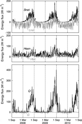
Fig. 11. Daily values of the surface energy fluxes over the entire period.
Melt season
Over the entire 3 year period, the surface was melting 36% of the time. The main melt season was May–October, when 94% of all melt occurred. Averaged over all half-hourly intervals with melt, S net was the largest contributor of melt energy (51%). As a result of the prevailing cloudy conditions during the main melt season (Table 3), the contribution of L net to the melt was positive (7%). The turbulent fluxes together supplied the remainder of the melt energy, with 31% from H sen and 12% from H lat. The contribution of the subsurface heat flux was small and slightly negative (–1%).
Table 3. Mean values of meteorological quantities and surface energy fluxes for AWS-I for periods when the surface was melting. Values are given for the entire period of operation of AWS-I (All: 14 September 2007 to 18 August 2010) and for the three (almost) complete mass-balance years (1 October–30 September) in the operational period
Compared to the other two mass-balance years, the amount of melt in 2008 was low. Although the observations for 2010 only ran until 18 August, the available melt energy was almost as large as for 2008. Summer air temperatures in 2008 were considerably lower than in the other two years, and wind speeds were slightly lower (Table 3). As a result, the turbulent fluxes contributed less to the melt energy. Combined with lower S net, likely caused by cloudier conditions, the total melt in 2008 was almost 1 m w.e. lower than in 2009.
During the short period with a bare ice surface, melt was 2 m ice a-1 at AWS-I (Fig. 12). The surface height changes measured by the sonic rangers correspond well to the observations at the nearest NVE mass-balance stake. The total ice melt and the melt rate computed with the surface energy-balance model also match the observed height changes well.

Fig. 12. Daily values of surface height change measured by the sonic height rangers at AWS-I and at the nearby NVE stake and modelled ice melt.
Discussion
Comparison with southern Norway
Two multi-year records from AWSs are available for the glaciers Storbreen and Midtdalsbreen in southern Norway (Reference Andreassen, Van den Broeke, Giesen and OerlemansAndreassen and others, 2008; Reference Andreassen, Van den Broeke, Giesen and OerlemansGiesen and others, 2008; Fig. 1). In this section, we compare the seasonal cycles of the main meteorological variables and the surface energy fluxes at these locations with the results for Langfjordjøkelen.
As on Langfjordjøkelen, the AWS sites in southern Norway were situated in the ablation zone. The datasets were analysed with the same energy-balance model, but span different time periods (Table 4). The longwave radiation correction applied in this study was not included in previous studies. To allow for the best comparison, the analyses of the other datasets were repeated with the longwave radiation correction included. Since the measurement height differed at the three locations and varied with snow depth, atmospheric variables are compared at the standard measurement heights of 2 m (air temperature) and 10 m (wind speed). The measurements were extrapolated to standard heights using the vertical profiles of air temperature and wind speed calculated with the energy-balance model.
Despite its more northerly latitude, the seasonal cycles of air temperature and humidity (not shown) on Langfjordjøkelen are very similar to the observations on the two glaciers in southern Norway (Fig. 13). This is due to the lower elevation of the AWS site and its close proximity to the coast. The AWS sites on Storbreen and Langfjordjøkelen are more sheltered than on Midtdalsbreen, resulting in lower wind speeds. At all locations, wind speeds are maximum in winter and minimum in summer. The largest difference is found in the cloudiness; Langfjordjøkelen is the cloudiest of the three AWS locations. Furthermore, effective cloud optical thickness is maximum in autumn and winter in southern Norway, but maximum in summer and autumn on Langfjordjøkelen.

Fig. 13. Monthly average values of (left side) air and surface temperature (T a at 2 m and T s), wind speed (v at 10 m) and effective cloud optical depth (τ) and (right side) monthly average surface energy fluxes for Langfjordjøkelen, Storbreen and Midtdalsbreen.
While the seasonal cycles of air temperature and wind speed on Storbreen and Langfjordjøkelen are almost identical, the differences in cloudiness have a large effect on the surface energy fluxes (Fig. 13). During melt conditions, S net at AWS-I is approximately a factor of two smaller than at the other two locations (Table 4). Besides the larger cloud optical thickness on Langfjordjøkelen, this also results from lower solar irradiance over the melt season and a longer period with snow cover. A second effect of the thick cloud cover is that L net at AWS-I is the largest of the three AWSs, reaching considerably positive values in July and August. The seasonal cycles of the turbulent fluxes at AWS-I are comparable to those computed for the AWSs in southern Norway; values for Langfjordjøkelen generally lie between those for Storbreen and Midtdalsbreen. Due to the short period with a bare ice surface, the melt energy at AWS-I is maximum in August, slightly later than at the other sites. The total number of days with melt is similar at the three AWS sites in Norway.
Table 4. Mean values of the energy fluxes (W m−2) and relative contribution to surface melt (%, boldface numbers) for AWS-I and two AWSs in southern Norway. The values for Langfjordjøkelen* are from an experiment with incoming solar radiation for the latitude of Storbreen. t melt gives the percentage of the total time with surface melt. All values are rounded to the nearest integer. Dates are dd.mm.yy
Compared to the two locations in southern Norway, the relative contribution of S net to melt is considerably lower on Langfjordjøkelen. This could be due to its more northerly latitude, but also to cloudier conditions, more shading and later disappearance of the snow cover at the AWS site. Although the positive contribution by L net at AWS-I partly compensates for this difference, the turbulent fluxes are more important in the surface energy balance on Langfjordjøkelen than on Storbreen and Midtdalsbreen.
According to the results by Messel (1985), the contributions of the turbulent fluxes to surface melt on the maritime glaciers Ålfotbreen in southern Norway and Engabreen in northern Norway are larger than on Langfjordjøkelen. However, observations on these two glaciers did not cover the entire melt season and the energy-balance calculations were based on different methods. Since this inhibits a detailed comparison, the relatively smaller turbulent fluxes on Langfjordjøkelen cannot conclusively be ascribed to climatic differences.
Latitudinal effect on solar radiation
To isolate the effect of the glacier latitude on S net and the surface energy balance, we recalculated the surface energy fluxes for Langfjordjøkelen with incoming solar radiation for the latitude of Storbreen. Half-hourly values of the atmospheric transmissivity from the measurements at AWS-I were multiplied by S in,TOA for 61.60° N to obtain S in at the glacier surface. Whenever the atmospheric transmissivity could not be calculated because there was no sunlight at AWS-I, we used the mean value of 0.43 (Table 1). We also did not take into account possible changes in the shading of the AWS site for different sun angles. Since at these times solar radiation was small, both assumptions had a negligible effect on the results. Reflected solar radiation was calculated by multiplying the new incoming solar radiation by the surface albedo.
Monthly mean S in,TOA is up to 60 W m−2 larger at the latitude of Storbreen. Differences are largest in spring and autumn, while in June S in,TOA is slightly larger on Langfjordjøkelen as a result of the midnight sun. Averaged over the year, S in at the AWS site would be 15 W m−2 larger at the latitude of Storbreen, but since most radiation is reflected, the change in S net would only be 3 W m−2.
When solar radiation for the Storbreen latitude was used in the energy-balance calculations, total melt increased by 6%, while the number of half-hourly periods with melt did not change (Table 4). Net solar radiation during periods with melt increased by 6 W m−2, while the difference in S net between Storbreen and Langfjordjøkelen is 36 W m−2. The experiment shows that the latitudinal effect on solar radiation only marginally affects the absolute and relative contribution of S net to the energy balance. Differences resulting from cloud conditions and snow-cover duration are much larger.
Comparison with other studies
Several earlier studies have tabulated results from surface energy-balance studies on glaciers at similarly high latitudes (e.g. Reference OhmuraOhmura, 2001; Reference De Woul and HockHock, 2005; Reference Giesen, Andreassen, Van den Broeke and OerlemansGiesen and others, 2009) and we refer to these studies for details. Since the locations of the measurement sites, the measurement periods and the methods used differ widely, only a general comparison is possible.
The 58% contribution of net radiation R net (S net + L net) to the surface energy balance on Langfjordjøkelen lies within the range of values found on glaciers at 65–75° N. Reported values range from ~ 40% on Engabreen, northern Norway (Reference Messel, Roland and HaakensenMessel, 1985), to 74% on McCall Glacier, Alaska, USA (Reference Klok, Nolan and Van den BroekeKlok and others, 2005). Similar values to Langfjordjøkelen are reported for Kårsa glacier (60%; Reference WallénWallén, 1948) and Storglaciären (66%; Reference Hock and HolmgrenHock and Holmgren, 1996) in northern Sweden, which also have comparable relative contributions by the sensible and latent heat fluxes. These two glaciers are situated further south and further inland than Langfjordjøkelen, where R net is expected to be more dominant in the energy balance. The inclusion of melt in spring for Langfjordjøkelen, when the contribution of R net is relatively large, may explain why the difference is rather small. Other glaciers with similar relative contributions by the surface energy fluxes to those at Langfjordjøkelen are Ecology Glacier, King George Island, Antarctica (Reference BintanjaBintanja, 1995), and West Gulkana Glacier, Alaska (Reference Brazel, Chambers and KalksteinBrazel and others, 1992), both glaciers with a maritime influence.
Few studies list the separate contributions by S net and L net, often because only R net was measured. Reported values for L net are always negative, so the positive contribution by L net found for Langfjordjøkelen is remarkable. Positive values for L net can only occur under warm, cloudy skies and may be characteristic for glaciers at low elevations in maritime environments. Note that the correction of the L in measurements for air temperatures above 0°C increased L net by several W m−2 for all three AWS sites in Norway. We recommend the inclusion of this correction in the analyses of AWS records from locations with air temperatures well above 0°C and where radiation measurements are made well above the surface.
Conclusions
We analysed a 3 year record from an AWS in the ablation zone of Langfjordjøkelen, northern Norway. Despite its location north of the polar circle, the glacier experiences a maritime climate. The annual mean air temperature at the AWS site was close to the melting point and even in midwinter, daily mean temperatures above 0°C were not uncommon. The air was humid year-round, with an average relative humidity above 80% in all three years and only occasional daily values below 50%. Frequent cloud cover combined with topographic shading reduced the amount of solar radiation at the top of the atmosphere by more than a factor of two before it reached the glacier surface. Snow covered the surface around the AWS from late September or early October until late July, with maximum snow depths above 3.5 m in all three years.
Over the 3 year period, 6 m of ice melted at the AWS site during the short periods without snow cover. The main melt season runs from May to October, but even in the dark winter months, melt occasionally occurred on warm, cloudy days. Net solar radiation provided the majority of the melt energy (51%), despite the high northern latitude of Langfjordjøkelen, the cloudy conditions and the short period with a low surface albedo. The remainder of the melt energy was supplied by the sensible and latent heat fluxes (31% and 12% respectively) and net longwave radiation (7%).
The seasonal cycles of most meteorological variables at the AWS site on Langfjordjøkelen are similar to measurements at two AWSs in southern Norway. However, cloud conditions are different, with more frequent and thicker clouds on Langfjordjøkelen, especially in summer. The contribution of net solar radiation to the melt energy is considerably lower on Langfjordjøkelen than in southern Norway. This is a combined effect of the thicker clouds and a later disappearance of the snow cover; the higher latitude of Langfjordjøkelen only plays a marginal role. Net longwave radiation during melt conditions is positive and slightly larger than at the two sites in southern Norway. The turbulent fluxes at Langfjordjøkelen have values comparable to southern Norway, but because of the smaller net solar radiation their relative contribution to the melt is larger.
The relative importance of net radiation for surface melt on Langfjordjøkelen is slightly smaller than values reported for glaciers in northern Sweden and considerably larger than values found in studies on other coastal glaciers in northern and southern Norway. However, the periods of investigation and the methods used to calculate the surface energy fluxes differ widely. It is therefore impossible to place the results for Langfjordjøkelen in the context of the regional gradients in net radiation found in previous studies. Additional multi-year records from both coastal and inland glaciers are needed to better resolve such patterns.
Acknowledgements
We thank technicians Wim Boot (IMAU) and Frode Kvernhaugen (NVE) for dedicated maintenance of AWS-I and AWS-N, and Bjarne Kjøllmoen (NVE) for providing stake data. This work was partly funded by the Research Council of Norway through the International Polar Year project Glaciodyn (2007–10). This publication is also contribution No. 34 of the Nordic Center of Excellence SVALI ‘Stability and Variations of Arctic Land Ice’ funded by the Nordic Top-level Research Initiative (TRI).


