


Introduction
Glacial landform assemblages left behind by Pleistocene ice sheets of North America and Northern Europe provide information on palaeo ice-sheet dynamics (Stokes and Clark, Reference Stokes and Clark1999; Stokes, Reference Stokes2018). Certain ice–bed conditions and processes can be derived from landform assemblages and compared to those operating in present-day ice sheets (e.g. landform elongation ratios and ice velocity; Kleman and others, Reference Kleman, Hättestrand, Borgström and Stroeven1997; Stokes and Clark, Reference Stokes and Clark2001; Stokes, Reference Stokes2018). Landform assemblages can also be used to reconstruct palaeo-ice sheets (e.g. Hughes and others, Reference Hughes, Clark and Jordan2014) and as analogues for current ice-sheet beds (Evans and others, Reference Evans, Archer and Wilson1999; Clark and others, Reference Clark, Hughes, Greenwood, Jordan and Sejrup2012; Bradwell and Stoker, Reference Bradwell and Stoker2015). An advantage of studying palaeo-ice sheets is that their former beds are visible and can be analysed with high-resolution digital elevation models (DEMs; e.g. Dowling and others, Reference Dowling, Spagnolo and Möller2015; Margold and others, Reference Margold, Stokes and Clark2015). In contrast, access to the bed of present-day ice sheets is restricted (Fretwell and others, Reference Fretwell2013), and relies on sparse boreholes and remote-sensing methods such as seismic surveys and radio-echo sounding (RES). Such data are commonly of low resolution and are acquired in widely spaced (≥500 m) flight lines (e.g. Bingham and others, Reference Bingham, Siegert, Young and Blankenship2007; Rippin and others, Reference Rippin2014; King and others, Reference King, Pritchard and Smith2016). This means that over large parts of present-day ice sheets there are uncertainties on sediment cover (Kulessa and others, Reference Kulessa2017), thermal state (MacGregor and others, Reference MacGregor2016), bed-elevation (Fretwell and others, Reference Fretwell2013) and bed-roughness (Bingham and Siegert, Reference Bingham and Siegert2009; Falcini and others, Reference Falcini, Rippin, Krabbendam and Selby2018; Cooper and others, Reference Cooper, Jordan, Siegert and Bamber2019). Although many definitions of bed roughness exist (Smith, Reference Smith2014), we define subglacial bed-roughness in this paper as the vertical variation of terrain over a given horizontal distance (Rippin and others, Reference Rippin2014). The roughness of subglacial topography, especially at shorter length-scales, affects drag at the ice– interface and is a primary control on basal sliding speeds, alongside effective water pressure and basal ice temperature (Schoof, Reference Schoof2002; Siegert and others, Reference Siegert, Taylor and Payne2005; Rippin, Reference Rippin2013). Uncertainties in bed-roughness measurements and in how ice flows over obstacles means that roughness in general is not taken into account in ice-sheet modelling, despite its probable importance (Bingham and others, Reference Bingham2017; Nias and others, Reference Nias, Cornford and Payne2016; Leong and Horgan, Reference Leong and Horgan2020).
Many previous studies have measured bed-roughness for both contemporary (RES data) and palaeo-ice-stream (DEMs) beds at scales that were too large (transect spacing of 30–50 km, along-transect resolution of 1.85 km–75 m and window sizes of 320 m–70 km) to capture glacial landforms (Siegert and others, Reference Siegert, Taylor, Payne and Hubbard2004; Rippin and others, Reference Rippin, Bamber, Siegert, Vaughan and Corr2006; Bingham and others, Reference Bingham, Siegert, Young and Blankenship2007; Rippin and others, Reference Rippin2014; Lindbäck and Pettersson, Reference Lindbäck and Pettersson2015). Yet, an increasing number of studies have demonstrated that small-scale glacial landforms exist underneath contemporary-ice sheets (e.g. King and others, Reference King, Woodward and Smith2007, Reference King, Hindmarsh and Stokes2009; Jezek and others, Reference Jezek2011; Bingham and others, Reference Bingham2017). These high-resolution (e.g. ≤500 × ≤500 m line spacing and ≤7.5 m along track spacing) studies, however, only cover small areas of contemporary-ice-stream beds, providing an incomplete analysis of landform location and distribution. It has not been feasible to expand these high-resolution studies across an entire contemporary-ice sheet due to the technical, cost and time constraints (see methods in King and others, Reference King, Pritchard and Smith2016). Recent study by Holschuh and others (Reference Holschuh, Christianson, Paden, Alley and Anandakrishnan2020) suggests future studies will be able to map larger areas at high resolution using airborne radar.
Palaeo-ice-sheet beds commonly have a complex and diverse range of landforms from drumlins to mega scale glacial lineations (MSGLs) (Stokes and Clark, Reference Stokes and Clark2001; Krabbendam and others, Reference Krabbendam, Eyles, Putkinen, Bradwell and Arbelaez-Moreno2016; Clark and others, Reference Clark2018b). Palaeo-ice-sheet beds provide an opportunity to measure bed roughness not just at the ice-stream scale (e.g. Gudlaugsson and others, Reference Gudlaugsson, Humbert, Winsborrow and Andreassen2013; Lindbäck and Pettersson, Reference Lindbäck and Pettersson2015; Falcini and others, Reference Falcini, Rippin, Krabbendam and Selby2018) but also at the landform scale. Yet, why should we measure bed roughness of glacial landform assemblages? If certain types of glacial landform assemblages have a range of bed-roughness values that are characteristic to them (bed-roughness signature), such information could be used to infer where landforms occur underneath contemporary-ice sheets (Stokes, Reference Stokes2018). This would improve our understanding of contemporary-ice-sheet beds, for example, by providing information on landform types, sediment cover vs hard-beds, sliding velocity (e.g. King and others, Reference King, Woodward and Smith2007), whether landforms are in a steady state (Hillier and others, Reference Hillier, Smith, Clark, Stokes and Spagnolo2013) or represent previous ice dynamics, and could also improve palaeo-ice-sheet models.
In this study, we investigate whether certain glacial landforms assemblages have characteristic bed-roughness signatures. We choose four study areas, all in the UK, each with a uniform glacial landform assemblage i.e. only one type of landform. These include cnoc and lochan, drumlins, megagrooves, and MSGLs. We also choose two areas that have mixed glacial landforms. The bed roughness of all six areas is quantified along sections parallel and orthogonal to palaeo-ice flow (1-D), and bed-roughness anisotropy is calculated from these 1-D results. Additionally, bed roughness is quantified using a 2-D method. We test whether uniform glacial landform assemblages have characteristic bed-roughness signatures i.e. can be differentiated from areas of mixed glacial landform assemblages, using both bed roughness and anisotropy of bed-roughness measurements.
Study areas and data
The British and Irish ice sheet (BIIS) was located on the edge of the Eurasian ice sheet complex (Hughes and others, Reference Hughes, Clark and Jordan2014), and was active during the Devensian 116–11.5 ka BP (Clark and others, Reference Clark, Hughes, Greenwood, Jordan and Sejrup2012). The Last Glacial Maximum (LGM) for the BIIS occurred between 30 and 21 ka BP, with retreat and readvance during 19–17 ka BP (Chiverrell and Thomas, Reference Chiverrell and Thomas2010), followed by final deglaciation around 14–13 ka BP (Clark and others, Reference Clark, Hughes, Greenwood, Jordan and Sejrup2012). Evidence from ice-rafted debris (e.g. Peck and others, Reference Peck2006), numerical modelling (e.g. Hubbard and others, Reference Hubbard2009) and ice flow set patterns (e.g. Hughes and others, Reference Hughes, Clark and Jordan2014), indicates that the BIIS was often unstable, with pronounced and repeated ice advances and retreats. Adjustments to these instabilities left behind landforms that have a complicated formation history as shown by cross cutting or overprinting features (Livingstone and others, Reference Livingstone, Ó Cofaigh and Evans2008, Reference Livingstone, Ó Cofaigh and Evans2010; Davies and others, Reference Davies2019). Over 170 000 landforms have been mapped from the BIIS (Clark and others, Reference Clark2018a), including areas, which are categorised as ‘classic’ glacial landform assemblages e.g. drumlin swarms.
The high-resolution NEXTMap Digital Terrain Model (DTM) was used to extract elevation data required for bed-roughness calculations. The NEXTMap DTM has a 5 m horizontal resolution and a 1 m vertical resolution (Bradwell, Reference Bradwell2013). The DTM tiles were downloaded from the Centre for Environmental Data Analysis (CEDA) Archive (Intermap Technologies, 2009). Landform distribution was assessed using BRITICE version 2.0 (Clark and others, Reference Clark2018a).
Study areas were chosen within the UK that had classic examples of uniform (one type) landforms i.e. cnoc and lochan, drumlins, megagrooves and MSGLs (areas 1–4, Figs 1c–f, Table 1). Individual landforms had to be large enough to be visible on NEXTMap DTM (>5 m wide and long, and >1 m high), so landforms at the meso- (1 m–1 km) and macro-scale (1 km–100 km) categories (Bennett and Glasser, Reference Bennett and Glasser2009) were selected. For areas of uniform landforms, our selection criteria required that the landforms have a single palaeo-ice-flow direction and no (or few) other landforms occurred in the study area. In addition, two areas were chosen that had a mix of different landforms, one in an upland and one in a lowland setting, to test whether uniform and mixed areas of glacial landforms can be differentiated from each other (areas 5 and 6, Figs 1g–h, Table 1).
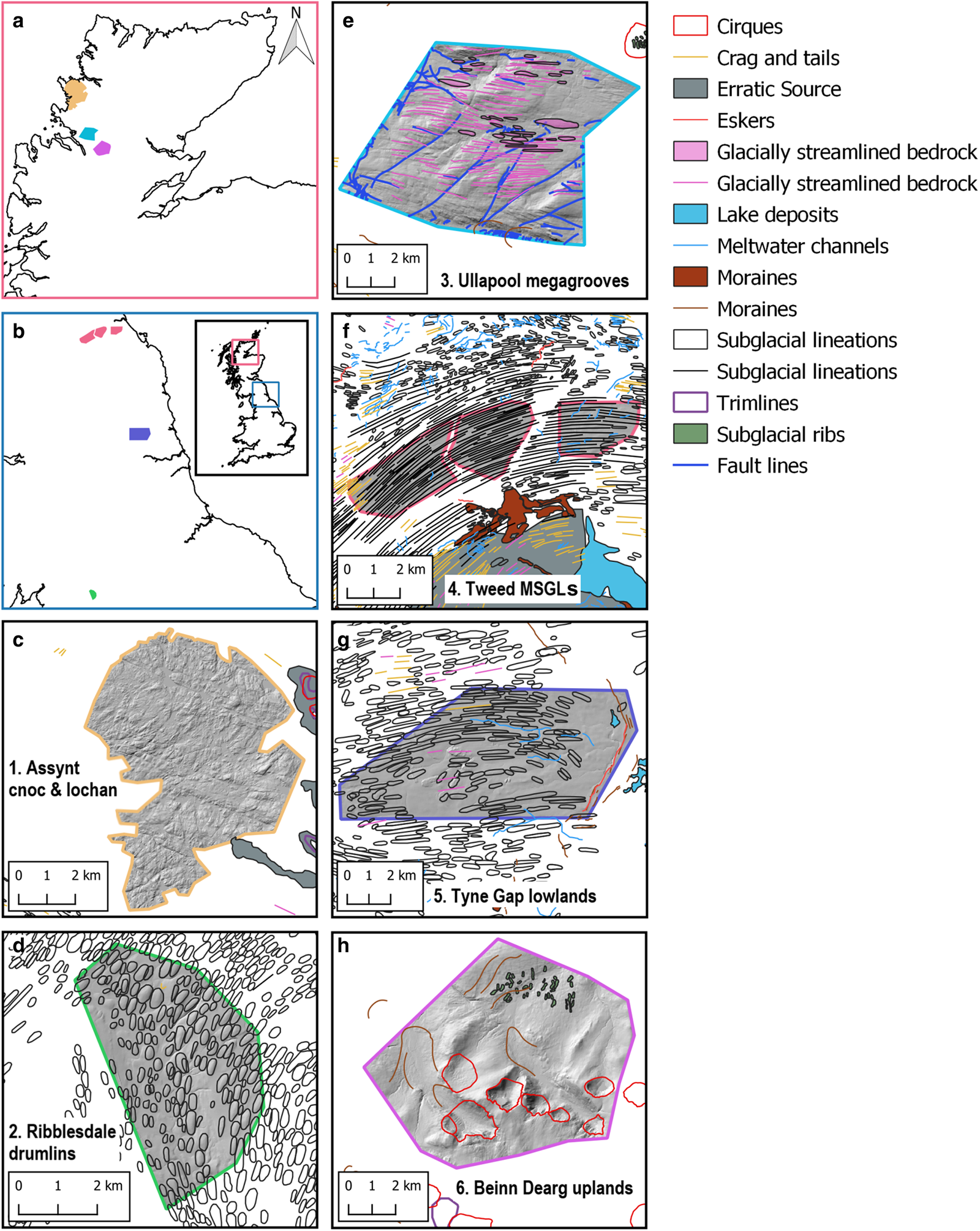
Fig. 1. (a), (b) Location of study areas (inset map in b). (a) Location of (c), (e), (h), while (b) shows (d), (f), (g). Each area is shown with NEXTmap DTM (Intermap Technologies, 2009) overlain by Britice glacial landforms (Clark and others, Reference Clark2018a). (c) Site 1: Assynt. Palaeo-ice flow was ≈ east to west. (d) Site 2: Ribblesdale. Palaeo-ice flow was ≈ northeast to southwest. (e) Site 3: Ullapool. Palaeo-ice flow was ≈ east to west. (f) Site 4: Tweed. Palaeo-ice flow was ≈ west to east. (g) Site 5: Tyne Gap. Palaeo-ice flow was ≈ west to east. (h) Site 6: Beinn Dearg. Palaeo-ice flow was ≈ east to west.
Table 1. Area information
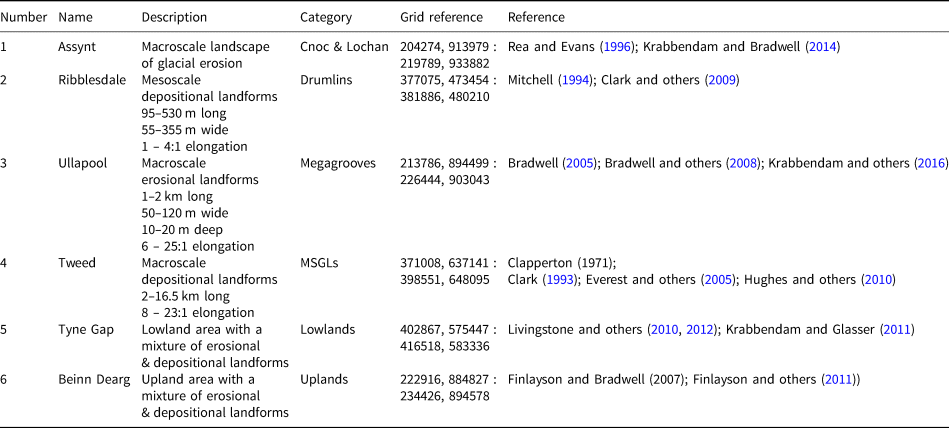
Descriptions include size and elongation ratios of the landforms where available from the literature.
Methods
In glaciology, bed-roughness is often calculated using fast Fourier transform analysis (FFT; e.g. Taylor and others, Reference Taylor, Siegert, Payne and Hubbard2004; Li and others, Reference Li2010; Spagnolo and others, Reference Spagnolo2017) or using standard deviation (SD; e.g. Rippin and others, Reference Rippin2014; Cooper and others, Reference Cooper, Jordan, Siegert and Bamber2019). These methods provide a statistical analysis of the vertical variation of elevation along a transect (Cooper and others, Reference Cooper, Jordan, Siegert and Bamber2019). Both FFT analysis and SD produce similar spatial distributions of bed-roughness values (Rippin and others, Reference Rippin2014; Falcini and others, Reference Falcini, Rippin, Krabbendam and Selby2018). An advantage of SD is that bed-roughness values are calculated in units of distance i.e. metres, (Cooper and others, Reference Cooper, Jordan, Siegert and Bamber2019) and it requires fewer data processing steps. We chose the SD method to quantify bed roughness in 1-D and 2-D. The 1-D approach measures bed roughness along transects – both parallel and orthogonal to the palaeo-ice flow – that sample the NEXTMap DTM. The 2-D approach measures bed roughness within a moving window (with a specific area and shape) centred at every pixel of the data domain. We used both approaches to assess which provided the clearest bed-roughness signatures.
1-D method for determining roughness
The 1-D method analyses along-transect elevation variations and thus imitates the data used to calculate bed roughness underneath contemporary ice streams as derived from RES surveys (i.e. grids of transects) (e.g. Siegert and others, Reference Siegert, Taylor, Payne and Hubbard2004; Bingham and others, Reference Bingham, Siegert, Young and Blankenship2007; Falcini and others, Reference Falcini, Rippin, Krabbendam and Selby2018). Transect grids with 5 m × 5 m spacing were created (ArcMap, ‘Create Fishnet’ tool) and rotated so that the transects were aligned approximately parallel and orthogonal to palaeo-ice flow (Fig. 2). The orientation of transects relative to ice flow has a clear effect on bed-roughness calculations: transects parallel to ice flow commonly give considerably lower roughness values than transects orthogonal to ice flow (Bingham and others, Reference Bingham2017; Falcini and others, Reference Falcini, Rippin, Krabbendam and Selby2018; Cooper and others, Reference Cooper, Jordan, Siegert and Bamber2019). This can be attributed to ice flow streamlining of the bed; a clear link with fast ice-surface velocity and smooth beds parallel but not orthogonal to flow was found by Cooper and others (Reference Cooper, Jordan, Siegert and Bamber2019). Ice-flow direction was interpreted from landform orientations (Stokes and Clark, Reference Stokes and Clark1999). Ice-flow direction is not necessarily in a straight line over a given distance. For example, ice flow is curved at areas 2 and 4 (Figs 1d, f). At area 4 the ice-flow curvature was overcome as the study area was easily split, but it was not possible in area 2. Area 6 also has complicated flow directions: during the LGM flow direction was approximately east to west, but in the Younger Dryas a plateau ice cap formed and ice flow was strongly topographically constrained with variable ice-flow directions (Finlayson and others, Reference Finlayson, Golledge, Bradwell and Fabel2011). The transects were positioned approximately east to west to match the dominant flow direction of the last BIIS because this larger ice mass likely had more impact on the roughness values.
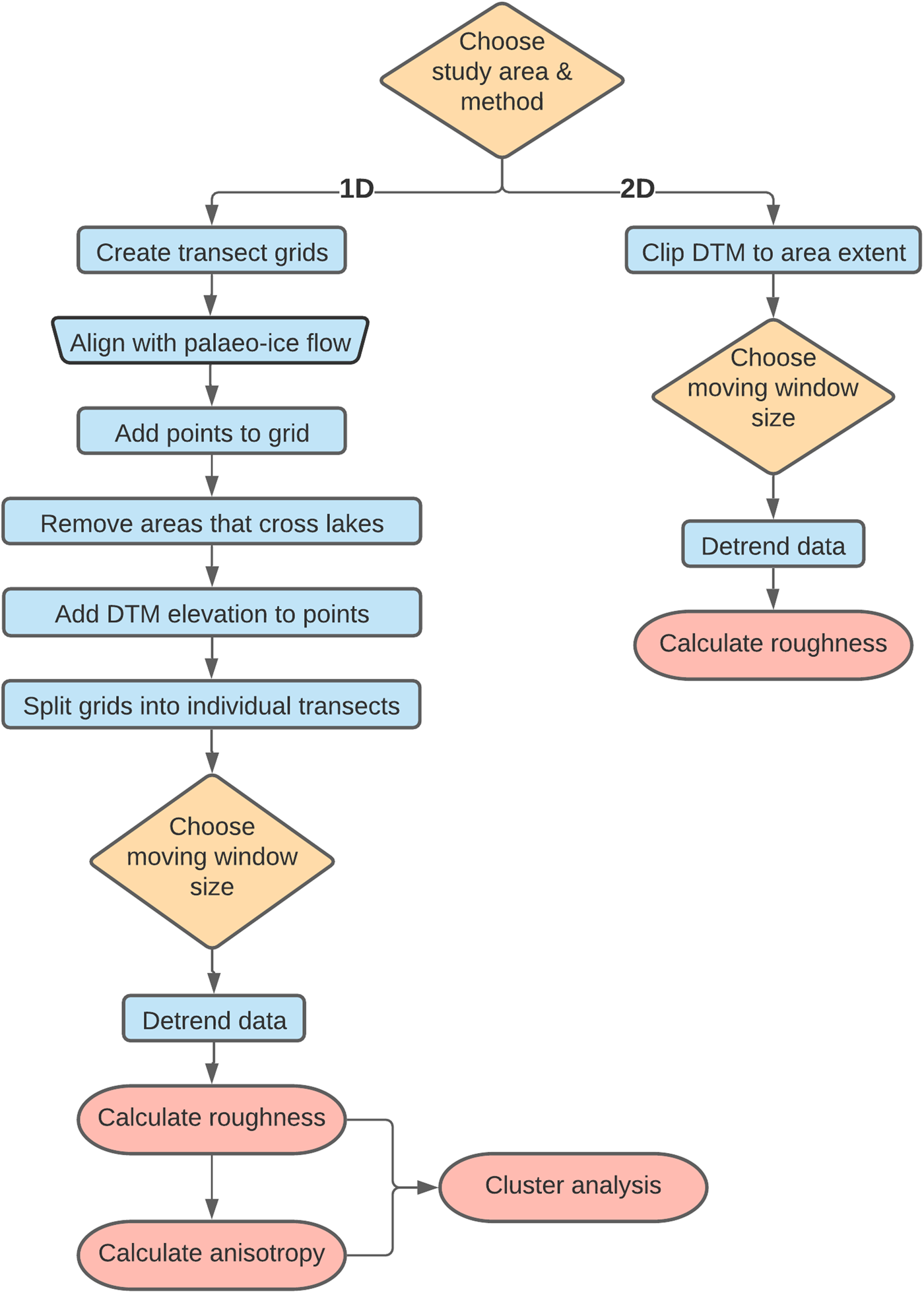
Fig. 2. Flow chart detailing the steps required to calculate bed roughness using both the 1-D and 2-D methods described in the ‘Methods’ section.
Points were added along the transects at 5 m intervals (QGIS, ‘QChainage’ plugin) to match the resolution of the NEXTMap DTM (Fig. 2). Areas that crossed lakes (OS Meridian 2 Lake shapefile) were removed to reduce a smoothing bias in the bed-roughness calculations (Gudlaugsson and others, Reference Gudlaugsson, Humbert, Winsborrow and Andreassen2013; Falcini and others, Reference Falcini, Rippin, Krabbendam and Selby2018). The NEXTMap DTM pixel values (elevation) were extracted and added to the grid point shapefiles, which were then split into individual transects. This enables bed roughness to be calculated separately for parallel and orthogonal to ice-flow transects.
Roughness is strongly scale dependent: a region of ‘flat’ terrain can be rough on the small scale, whereas a high-relief landscape can be smooth on the large scale (Shepard and Campbell, Reference Shepard and Campbell1999; Prescott, Reference Prescott2013). Due to the size variation of landforms, moving windows of 100 m and 1 km were chosen to capture bed-roughness signatures at a range of scales (Table 1). Before bed-roughness was calculated, the data were detrended (Fig. 2) to remove large wavelengths caused by mountains and valleys, which would otherwise dominate the bed-roughness values (Shepard and others, Reference Shepard2001; Smith, Reference Smith2014). The data were detrended by calculating the mean for each point along a transect within a moving window (100 m and 1 km) and subtracted from the original to leave the detrended output. SD of elevation was then calculated along every transect using the same moving window sizes that were used for detrending. The transects were then combined and converted to a raster for easier display.
Anisotropy (directionality) calculation
Anisotropy (also referred to as directionality; Rippin and others, Reference Rippin2014) is a useful metric for interpreting bed-roughness measurements as it quantifies the difference between roughness parallel ($R_\parallel$ ) and roughness orthogonal (R ⊥) to ice flow (Smith, Reference Smith2014). Anisotropy can only be calculated at points where parallel and orthogonal transects cross, which is why we created 1-D transects from 2-D raster DTMs. Using the transect grids created in section ‘1-D method for determining roughness’, the anisotropy ratio (Ω) was calculated using the following equation from Smith and others (Reference Smith, Raymond and Scambos2006):

where when $R_\parallel$ is the roughness of a transect parallel to ice flow and R ⊥ is the roughness orthogonal to ice flow. Anisotropy Ω is closer to 1 when $R_\parallel$
 is higher than R ⊥, is 0 when bed roughness is isotropic, and closer to −1 when R ⊥ is higher than $R_\parallel$
 . Note that anisotropy Ω is zero both on a perfect smooth plane, but also in a very rough, but truly random landscape.
2-D method
The 2-D method uses the NEXTMap DTM data in raster format i.e. no transects were created. The NEXTMap DTM (elevation data) was clipped to the extent of all the study areas (Fig. 2). The clipped raster was then detrended by calculating mean elevation rasters (ArcMap, ‘Focal Statistics’ tool) and then subtracting these from the original DTM. Similar to the 1-D method, window sizes of 100 m and 1 km were used to capture roughness at two scales. SD of elevation was calculated for the detrended rasters using a moving window (same size as used for detrending, 100 m and 1 km).
Cluster analysis
To further test whether bed roughness and anisotropy data from the areas fall into landform groups, cluster analysis was carried out. Cluster analysis places data into groups (the number of groups is specified by the user). This is done by placing each individual data point into a group that has the nearest centroid (multidimensional equivalent of the mean; Crawley, Reference Crawley2007). We used the partitioning based K-means cluster analysis function in R, which uses the algorithm developed by Hartigan and Wong (Reference Hartigan and Wong1979). The variables used were bed-roughness (mean values calculated from the parallel and orthogonal transect crossover locations) and anisotropy across individual areas. For each window size, cluster analysis was calculated for areas 1–4 and 6, and then just for areas 1–4 to establish if the uniform landform types could be grouped more easily without the mixed area. Area 5 was not included due to striping in the anisotropy data (see ‘Striping error’ section). The bed roughness and anisotropy data used were from the interquartile range. Statistics on how well the cluster analysis performed when compared to the landform groupings were calculated using the confusion Matrix function in R, and are reported in the figure captions.
Results
Area 1: Assynt cnoc and lochan landscape
The cnoc and lochan landscape of Assynt in NW Scotland (Fig. 1) is a macroscale landscape of glacial erosion, characterised by abundantly exposed bedrock with numerous hills (cnocs), lakes (lochan) and small valleys. The landscape is typical for glacially eroded basement or ‘shield’ terrain (Rea and Evans, Reference Rea and Evans1996; Krabbendam and Bradwell, Reference Krabbendam and Bradwell2014).
The cnoc and lochan landscape is somewhat rougher orthogonal to palaeo-ice-flow direction rather than parallel to it (Figs 3a–d). The cnoc and lochan has low anisotropy values, with a mean of −0.1 for the 1 km window values and 0 for the 100 m window values (Table 2). The roughest locations (red areas) calculated using a 1 km window (Figs 3a, c, g) are not picked up when using a 100 m window (Figs 3b, d, h). These areas are located over bedrock highs with steep slopes. The roughest locations (red areas) calculated using a 100 m window are located at lake edges and existing faults lines (Figs 3b, d, h).
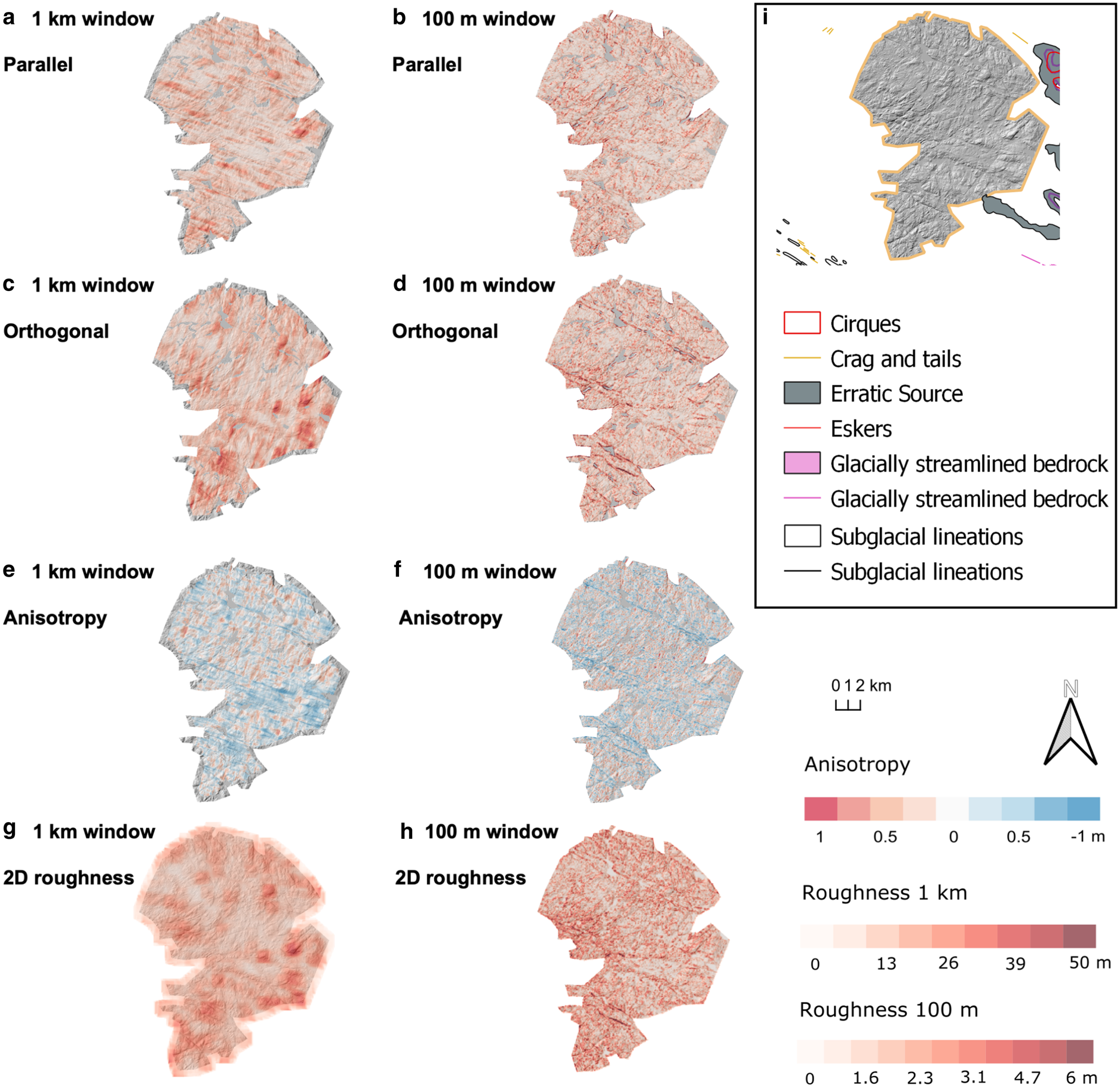
Fig. 3. Bed roughness over the Assynt cnoc and lochan (area 1). Bed roughness was calculated parallel (a, b) and orthogonal (c, d) to palaeo-ice flow direction (1-D), and for all flow directions (2-D; g, h), using SD with 1 km and 100 m window sizes. (e, f) Anisotropy of bed roughness was calculated at the crossover points between parallel and orthogonal transects for both window sizes. Between − 1 and 0, orthogonal -roughness values dominate (blue). Between 0 and 1, parallel bed-roughness values dominate (red). At 0, bed roughness is isotropic (white). (i) Location area from Fig. 1 overlain with glacial landforms for comparison.
Table 2. Statistics of bed roughness and anisotropy for all areas (m)
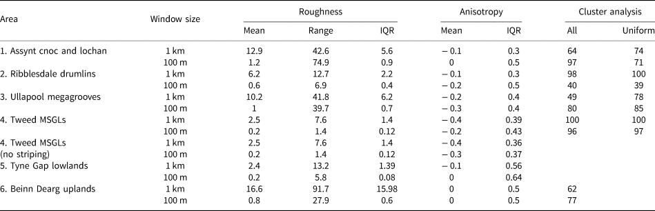
The statistics were calculated by combining values for both flow directions. Two sets of values were reported for the Tweed due to the striping in the anisotropy; one for the whole site, and one without the eastern section that has the striping. IQR = interquartile range. Accuracy of the cluster analysis is reported (%) for all sites analysed and where only the uniform landform assemblages were analysed (Figs 8 and 9).
Area 2: Ribblesdale drumlins
The Ribblesdale drumlins of the Yorkshire Dales (Fig. 1) have been described as ‘classically shaped’ because they are half egg-shaped features, which appear as blisters superimposed on the landscape (Clark and others, Reference Clark2009; Spagnolo and others, Reference Spagnolo, Clark and Hughes2012). Drumlins are sediment and/or rock formed, smooth, oval-shaped hills and are categorised as mesoscale landforms (Menzies, Reference Menzies1979; Benn and Evans, Reference Benn and Evans2010). The drumlins in Ribblesdale have a length of 95–530 m, widths of 55–355 m and elongation ratios of 1–4 : 1 (Mitchell, Reference Mitchell1994; Clark and others, Reference Clark2009). Figures 3a–d show that the drumlin field is rougher orthogonal rather than parallel to the palaeo-ice-flow direction. The same spatial pattern is shown by the anisotropy values, with higher roughness values orthogonal to palaeo-ice flow (Figs 4e–f) and mean anisotropy values of −0.1 and −0.2 (Table 2). The roughest values are located over small post-glacial streams (Figs 4a—d, h), and thus arguably not relevant for the overall analysis. Individual drumlins can be seen more clearly using the 100 m window size, and have high bed-roughness values on the drumlin sides but not on the crests (Figs 4d, h). It should be noted that not all the drumlins are exactly aligned to the transects due to the slight curving of the ice-flow direction.
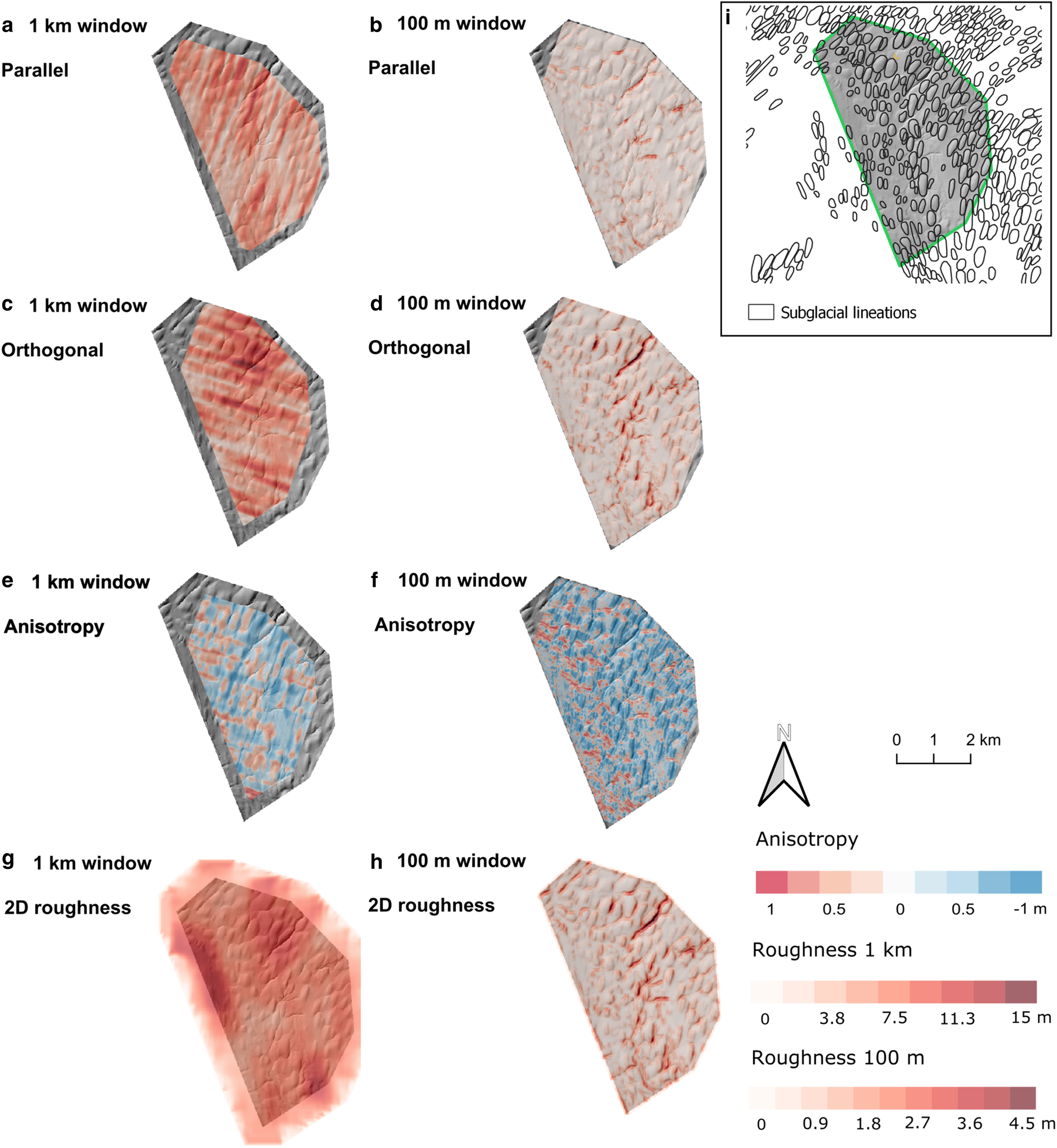
Fig. 4. Bed roughness over the Ribblesdale drumlins (area 2). Bed roughness was calculated parallel (a, b) and orthogonal (c, d) to palaeo-ice flow direction (1-D), and for all flow directions (2-D; g, h), using SD with 1 km and 100 m window sizes. (e, f) Anisotropy of bed roughness was calculated at the crossover points between parallel and orthogonal transects for both window sizes. Between −1 and 0, orthogonal bed-roughness values dominate (blue). Between 0 and 1, parallel bed-roughness values dominate (red). At 0, bed roughness is isotropic (white). (i) Location area from Fig. 1 overlain with glacial landforms for comparison.
Area 3: Ullapool megagrooves
The Ullapool megagrooves located in NW Scotland (Fig. 1) are erosional, macroscale landforms described as metre-scale deep grooves in rock, and are located in an area measuring 6 km by 10 km (Bradwell, Reference Bradwell2005; Krabbendam and others, Reference Krabbendam, Eyles, Putkinen, Bradwell and Arbelaez-Moreno2016; Newton and others, Reference Newton, Evans, Roberts and Stokes2018). The megagrooves have a typical length of 1000–2000 m, width of 50–120 m, depth of 10–20 m and elongation ratios of 6–25 : 1 (Bradwell and others, Reference Bradwell, Stoker and Krabbendam2008). The megagrooves are considerably rougher orthogonal to palaeo-ice-flow direction than parallel to the palaeo-ice-flow direction (Figs 5a–d). The anisotropy values support this observation (Figs 5e, f) with mean anisotropy between −0.2 and −0.4 (Table 2). Some pre-existing geological faults that are orientated diagonally across the megagrooves (Fig. 1e) can be seen in the parallel to palaeo-ice-flow and 2-D data (Figs 5a, b, h). Roughness along the transects orthogonal to ice flow is greater for deeper megagrooves (up to 6 m) than for shallower ones (up to 3 m).
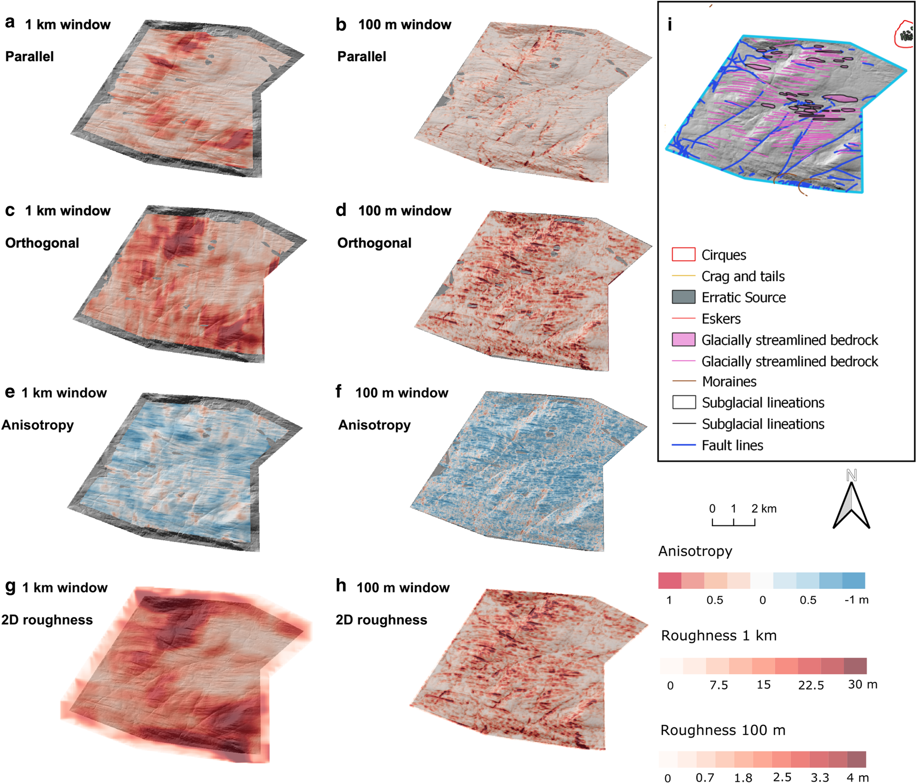
Fig. 5. Bed roughness over the Ullapool megagrooves (area 3). Bed roughness was calculated parallel (a, b) and orthogonal (c, d) to palaeo-ice flow direction (1-D), and for all flow directions (2-D; g, h), using SD with 1 km and 100 m window sizes. (e, f) Anisotropy of bed roughness was calculated at the crossover points between parallel and orthogonal transects for both window sizes. Between −1 and 0, orthogonal bed-roughness values dominate (blue). Between 0 and 1, parallel bed-roughness values dominate (red). At 0, bed roughness is isotropic (white). (i) Location area from Fig. 1 overlain with glacial landforms for comparison.
Area 4: Tweed MSGLs
The Tweed MSGL landsystem located in NE England (Fig. 1) comprises MSGLs: depositional, macroscale landforms formed at the base of the Tweed Palaeo-Ice Stream (Everest and others, Reference Everest, Bradwell and Golledge2005). MSGLs are described as very elongated ridges, which are spaced parallel to each other (Clark, Reference Clark1993; Spagnolo and others, Reference Spagnolo2014). The Tweed MSGLs are 2–16.5 km long and have elongation ratios of 8–23 : 1 (Everest and others, Reference Everest, Bradwell and Golledge2005; Hughes and others, Reference Hughes, Clark and Jordan2010).
Like the megagrooves and drumlins, the MSGLs in area 4 are rougher orthogonal rather than parallel to palaeo-ice-flow direction (Figs 6a–d). This is also shown by the anisotropy values (Figs 6e, f), with mean anisotropy values of −0.4 and −0.3 for the 1 km and 100 m windows, respectively (Table 2) being the highest of any area. Area 4 has the lowest mean roughness values compared to the other uniform landforms (areas 1–3; Table 2). The crests of the MSGLs are shown as rough by the parallel to palaeo-ice flow (for 1 km window size results; Fig. 6a), in contrast to drumlin crests.
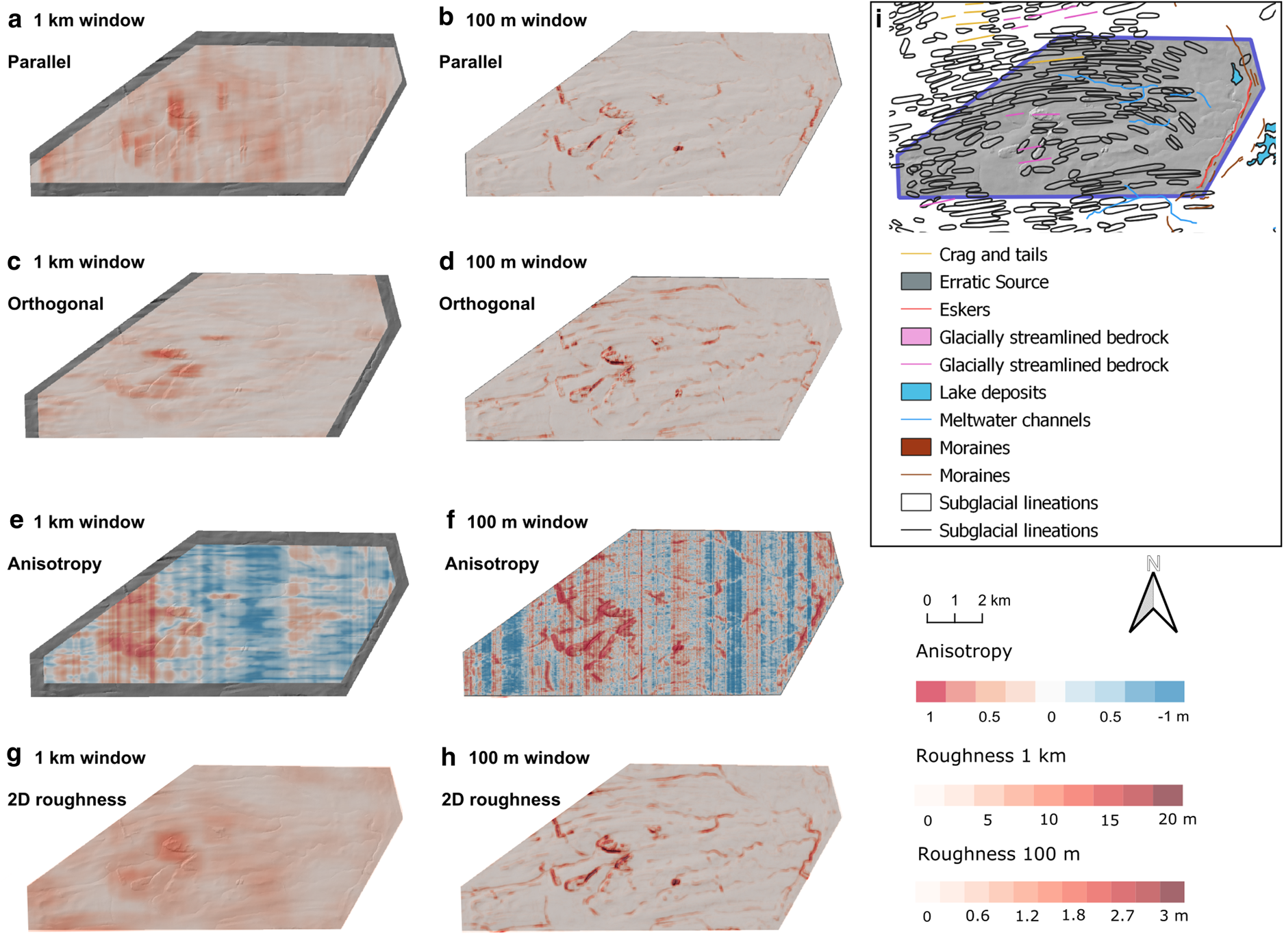
Fig. 6. Bed roughness over the Tweed MSGLs (area 4). Bed roughness was calculated parallel (a, b) and orthogonal (c, d) to palaeo-ice flow direction (1-D), and for all flow directions (2-D; g, h), using SD with 1 km and 100 m window sizes. (e, f) Anisotropy of bed roughness was calculated at the crossover points between parallel and orthogonal transects for both window sizes. Between − 1 and 0, orthogonal bed-roughness values dominate (blue). Between 0 and 1, parallel bed-roughness values dominate (red). At 0, bed roughness is isotropic (white). (i) Location area from Fig. 1 overlain with glacial landforms for comparison.
Area 5: Tyne Gap lowlands
Located in NE England (Fig. 1), area 5 is part of the Tyne Gap Palaeo-Ice Stream (Livingstone and others, Reference Livingstone2015), and is a lowland area that has a mix of depositional and erosional landforms (Krabbendam and Glasser, Reference Krabbendam and Glasser2011). Elongation ratios vary from 1–10 : 1 (Livingstone and others, Reference Livingstone, Ó Cofaigh and Evans2010, Reference Livingstone2012).
The bed-roughness results from the glaciated lowland area suggest that it is slightly rougher orthogonal rather than parallel to palaeo-ice-flow direction (Figs 7a–d). This is shown by the low anisotropy result (Figs 7e–f) for the 1 km window only, which has a mean value of −0.1. The 100 m window has a mean value of 0 and is isotropic (Table 2). The bed-roughness values for area 5 are similar to those from area 4, and these areas are the smoothest overall (Table 2). The roughest area (in red) shown in the 1 km window results is an area of exposed bedrock (Figs 1g, 7a, c), which is also shown as rough (red) for the 100 m window results, as are some of the meltwater channels (Figs 1g, 6b, d). The esker and moraines that are located at the far east of area 5 (Fig. 1g) are picked out as rough by the 100 m window data (Figs 7b, d) and have >0 anisotropy values (Fig. 7f). The majority of the drumlins (Fig. 1g) are not shown as rough on the 100 m window data (Figs 7b, d, h). Those that are rough appear to be rock cored (Livingstone and others, Reference Livingstone, Ó Cofaigh and Evans2008; Krabbendam and Glasser, Reference Krabbendam and Glasser2011).
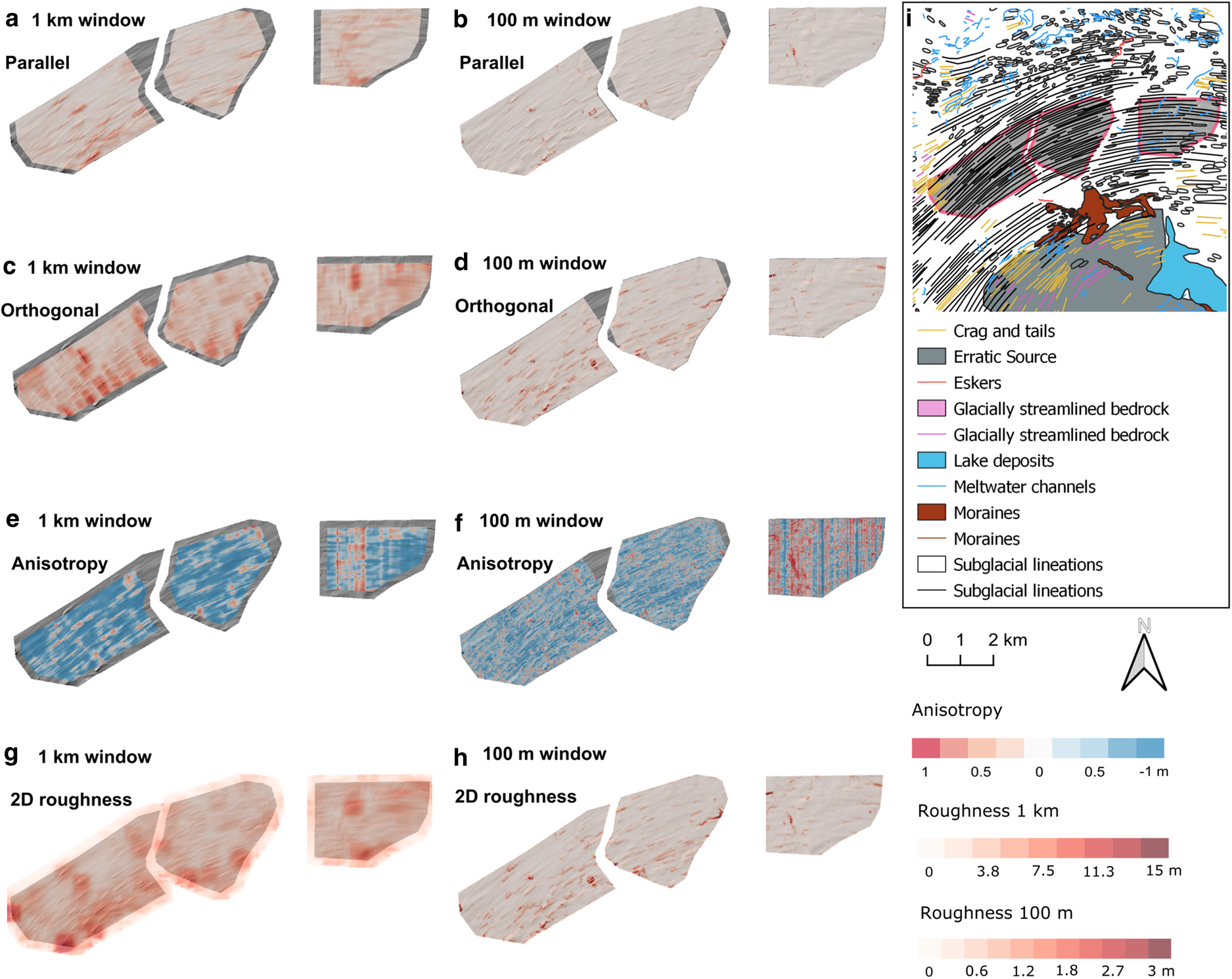
Fig. 7. Bed roughness over the Tyne Gap mixed lowlands (area 5). Bed roughness was calculated parallel (a, b) and orthogonal (c, d) to palaeo-ice flow direction (1-D), and for all flow directions (2-D; g, h), using SD with 1 km and 100 m window sizes. (e, f) Anisotropy of bed roughness was calculated at the crossover points between parallel and orthogonal transects for both window sizes. Between − 1 and 0, orthogonal -roughness values dominate (blue). Between 0 and 1, parallel bed-roughness values dominate (red). At 0, bed roughness is isotropic (white). (i) Location area from Fig. 1 overlain with glacial landforms for comparison.
Area 6: Beinn Dearg uplands
Located in Beinn Dearg massif, NW Scotland, area 6 is an upland area that has a mix of depositional and erosional landforms (Fig. 1 Finlayson and others, Reference Finlayson, Golledge, Bradwell and Fabel2011). This area comprises cirques and glacial valleys, as well as Rogen moraines (Hughes and others, Reference Hughes, Clark and Jordan2010; Finlayson and others, Reference Finlayson, Golledge, Bradwell and Fabel2011).
The mean anisotropy for both window sizes is 0 (Table 2), and there is no clear spatial pattern of anisotropy in relation to the glacial landforms (Figs 8e–f). The highest bed-roughness values (red) are found on the steep cirques (Figs 1h and 8a–d, g, h), which is expected. Both parallel and orthogonal to palaeo-ice flow results derived from a 100 m window size show the ribbed moraines as rougher than the surrounding areas (Figs 1h and 8b, d, h), but this is not shown by the 1 km window size results (Figs 8a, c, g) and cannot be seen in the anisotropy data (Figs 8e–f). In the 100 m window results, there are other features in close proximity to the rogen moraines that have similar roughness values and spatial patterns (Figs 8b, d). The origin of these features, which were not mapped by Clark and others (Reference Clark2018a) or Finlayson and others (Reference Finlayson, Golledge, Bradwell and Fabel2011), is not clear.
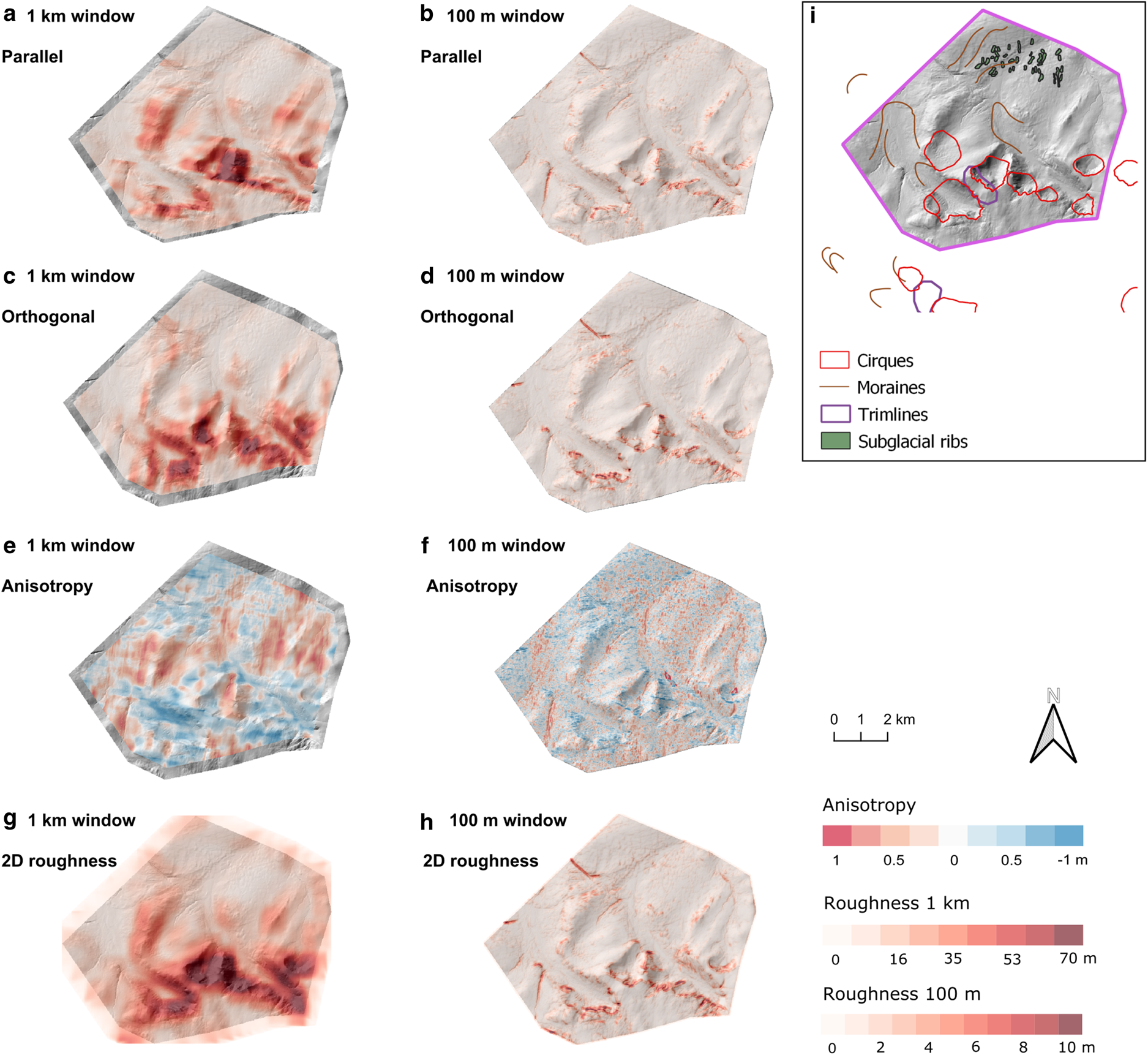
Fig. 8. Bed roughness over the Beinn Dearg mixed uplands (area 6). Bed roughness was calculated parallel (a, b) and orthogonal (c, d) to palaeo-ice flow direction (1-D), and for all flow directions (2-D; g, h), using SD with 1 km and 100 m window sizes. (e, f) Anisotropy of bed roughness was calculated at the crossover points between parallel and orthogonal transects for both window sizes. Between − 1 and 0, orthogonal -roughness values dominate (blue). Between 0 and 1, parallel bed-roughness values dominate (red). At 0, bed roughness is isotropic (white). (i) Location area from Fig. 1 overlain with glacial landforms for comparison.
Comparison of results
A summary of all the bed roughness and anisotropy data across the areas can be seen in Table 2. The MSGLs (area 4) are the most anisotropic and least rough of all the landforms at the 1 km window size scale (Table 2). The mixed uplands (area 6) is the roughest area at the 1 km window scale and is the only one that is isotropic with the 1 km window size (Table 2). At this window size, the cnoc and lochan and megagrooves areas (3 and 1) have very similar mean bed roughness and anisotropy values (Table 2). Using the 100 m window size, the megagrooves and cnoc and lochan areas can be distinguished more clearly with a large difference in anisotropy (− 0.3 vs 0; Table 2). At this window size, both cnoc and lochan and uplands areas (1 and 6) are isotropic, while all the other areas have a negative anisotropy (Table 2). The results from the cluster analysis show that the MSGLs (area 4) can be clearly grouped for both the 1 km window and 100 m windows (Figs 9 and 10); the accuracy of the cluster analysis (how accurate it is at placing values from the MSGLs in the same cluster group) is 100 and 96% respectively. The cluster analysis also shows that the cnoc and lochan and megagrooves areas (1 and 3) are better separated for the 100 m window results compared to the 1 km window results (Figs 9b, d, 10b, d). The accuracy for the cnoc and lochan and megagrooves areas (1 and 3) when groups 1–4 and 6 were used in the cluster analysis was 64 and 49% respectively for the 1 km window data (Fig. 9b), and 67 and 80% respectively for the 100 m window data (Fig. 10b). When the upland area (6) was removed from the cluster analysis, the accuracies for the cnoc and lochan and megagrooves areas (1 and 3) was 74 and 78% respectively for the 1 km window data (Fig. 9d), and 71 and 85% respectively for the 100 m window data (Fig. 10d). The accuracy for placing values correctly in the megagroove (area 3) cluster group is much better for the 100 m window compared to the 1 km window, but this is not the case for the cnoc and lochan (area 1). For the drumlins (area 2), the cluster analysis showed clear results for the 1 km window data with accuracies of 98 and 100% (Fig. 9b). However, for the 100 m window data, the cluster analysis had accuracies of 40 and 39% as there was a lot of crossover with other cluster groups (Fig. 10b).
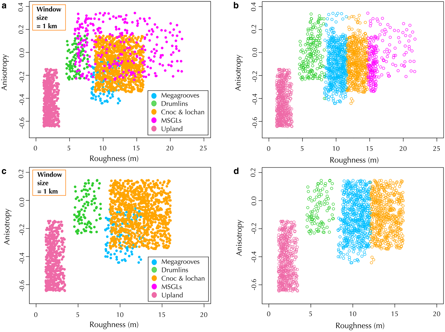
Fig. 9. Cluster analysis of bed roughness vs anisotropy for all areas except for area 5. (a) All the values derived using a 1 km window size colour coded by landform type (i.e. by area). (b) The results of cluster analysis. The cluster groups are colour coded to match the landform groups. The overall accuracy of the cluster analysis groups compared to the real landform groups was 58%. The accuracy for each area was 64% for area 1 (cnoc and lochan), 98% for area 2 (drumlins), 49% for area 3 (megagrooves), 100% for area 4 (MSGLs) and 62% for area 6 (Upland). (c) The same as (a) but only uniform landform sites were used (i.e. sites 1–4). (d) The same as (b) but only using the data from (c). The overall accuracy of the cluster analysis groups compared to the real landform groups was 71%. The accuracy for each area was 74% for area 1 (cnoc and lochan), 100% for area 2 (drumlins), 78% for area 3 (megagrooves) and 100% for area 4 (MSGLs).
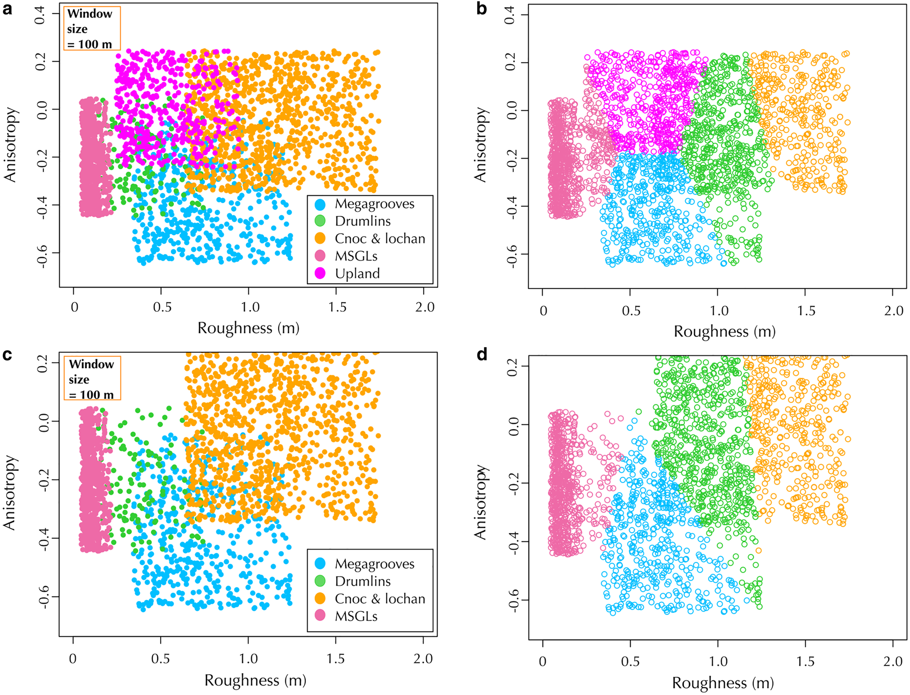
Fig. 10. Cluster analysis of bed roughness vs anisotropy for all areas except for area 5. (a) All the values derived using a 100 m window size colour coded by landform type (i.e. by area). (b) The results of cluster analysis. The cluster groups are colour coded to match the landform groups. The overall accuracy of the cluster analysis groups compared to the real landform groups was 60%. The accuracy for each area was 97% for area 1 (cnoc and lochan), 40% for area 2 (drumlins), 80% for area 3 (megagrooves), 96% for area 4 (MSGLs) and 77% for area 6 (Upland). (c) The same as (a) but only uniform landform sites were used (i.e. sites 1–4). (d) The same as (b) but only using the data from (c). The overall accuracy of the cluster analysis groups compared to the real landform groups was 65%. The accuracy for each area was 71% for area 1 (cnoc and lochan), 39% for area 2 (drumlins), 85% for area 3 (megagrooves) and 97% for area 4 (MSGLs).
Striping error
Due to the striping in the anisotropy results for the eastern section of area 4 (MSGL; Figs 6e, f) and area 5 (lowlands; Figs 7e, f), these data were not included in Table 2 or the cluster analysis to ensure they did not bias the results. The striping might be caused by the orientation of the transects. For these areas only, the transects are aligned exactly north south and east west, which is the same as the DTM pixel orientation. The striping is much more prevalent in the 100 m window results compared to the 1 km window results (e.g. Figs 7e vs 7f). Striping artefacts by their nature are anisotropic, and have been shown to be scale-dependent, having a greater effect on DTM curvature distributions at smaller window sizes (Sofia and others, Reference Sofia, Pirotti and Tarolli2013). The collection of DTM data along lines can cause striping artefacts during interpolation that can impact roughness results (Sofia and others, Reference Sofia, Pirotti and Tarolli2013; Trevisani and Cavalli, Reference Trevisani and Cavalli2016). NEXTMap DTM data were collected using parallel flight lines, with three orthogonal flight lines per 200 km × 200 km block to aid systematic error removal (Mercer, Reference Mercer2007). A visual inspection of the NEXTMap DTM shows that there is no striping at areas 4 and 5. Thus, this was an unexpected error, which was only visible in the anisotropy measurements. Transects should not be aligned with the DTM pixel direction to avoid this error.
Discussion
Roughness and anisotropy signal of landform assemblages
The results show that glacial landforms assemblages do have characteristic bed-roughness signatures when anisotropy values are used alongside bed-roughness measurements (Figs 9c and 10c, Table 2). Drumlin, megagroove and MSGL fields (areas 2, 3 and 4) show substantial anisotropy (≤ −0.2) compared to the cnoc and lochan (area 1) and mixed areas 5 and 6 (≥ −0.1). In most cases, anisotropy is negative, which is where bed roughness is higher orthogonal to palaeo-ice-flow direction (related to ice streamlining; Figs 9a and 10a). This type of anisotropy in essence describes elongation ratios of glacial landforms, which is thought to directly relate to streamlining and ice velocity (Stokes and Clark, Reference Stokes and Clark1999; Spagnolo and others, Reference Spagnolo2017). The megagrooves and MSGLs (areas 3 and 4) have a higher mean anisotropy compared to the drumlins, which is consistent with the reported elongation values (6-25 : 1, 8-23 : 1, and 1-4 : 1 respectively; Mitchell, Reference Mitchell1994; Everest and others, Reference Everest, Bradwell and Golledge2005; Bradwell and others, Reference Bradwell, Stoker and Krabbendam2008). The areas that have mixed landforms are more isotropic, compared to the areas of uniform landforms (areas 2, 3 and 4) that have clear elongation ratios. Along with studies that demonstrate the effect of transect orientation on bed-roughness results (e.g. Gudlaugsson and others, Reference Gudlaugsson, Humbert, Winsborrow and Andreassen2013; Rippin and others, Reference Rippin2014; Bingham and others, Reference Bingham2015; Falcini and others, Reference Falcini, Rippin, Krabbendam and Selby2018; Cooper and others, Reference Cooper, Jordan, Siegert and Bamber2019), these outcomes underline the importance of considering the anisotropy of bed roughness. Transects orientated parallel and orthogonal to ice flow are needed to calculate the anisotropy of bed roughness, and there are large datasets in Antarctica and Greenland that fit this criterion (e.g. Bingham and Siegert, Reference Bingham and Siegert2009; King and others, Reference King, Hindmarsh and Stokes2009; Rippin, Reference Rippin2013; Lindbäck and Pettersson, Reference Lindbäck and Pettersson2015; Bingham and others, Reference Bingham2017).
Both the megagrooves (area 3) and the cnoc and lochan (area 1) are underlain by hard bedrock, with very little sediment cover (Bradwell, Reference Bradwell2005; Bradwell and others, Reference Bradwell, Stoker and Krabbendam2008; Krabbendam and Bradwell, Reference Krabbendam and Bradwell2014). Using the 1 km window size, both areas show similar mean bed roughness and anisotropy (Table 2 and Fig 9c). Yet, at smaller roughness scales (100 m window), the results show a clear difference between the cnoc and lochan (area 1) and megagrooves (area 3) (Figs 9c and 10c), with the megagrooves being considerably more anisotropic than the cnoc and lochan terrain. This difference in anisotropy between areas 1 and 3 is linked to the underlying geology. The fracture and joints of the basement gneiss in Assynt (area 1 location) are in essence isotropic whereas sedimentary and metasedimentary rocks often have highly anisotropic bedding planes (Krabbendam and Bradwell, Reference Krabbendam and Bradwell2014), which can be preferentially eroded to form megagrooves (Krabbendam and Glasser, Reference Krabbendam and Glasser2011; Krabbendam and others, Reference Krabbendam, Eyles, Putkinen, Bradwell and Arbelaez-Moreno2016).
The MSGLs (area 4) have a higher anisotropy for the 1 km window results compared to the 100 m window results. The MSGLs (area 4) are the only uniform landform area where this occurs (Figs 9a and 10a). The MSGLs typically have a spacing between landforms of 200–800 m and can be more than 200 m wide (Bradwell and others, Reference Bradwell, Stoker and Krabbendam2008). Therefore, the bed-roughness signature is more distinct for the MSGLs (area 4) when using the 1 km window size because the 100 m window results may fall within the scale of an individual landform, and does not capture the roughness of the terrain as a whole.
The results indicate that a combination of bed roughness and bed-roughness anisotropy, can be used to differentiate uniform areas of landforms from each other, as well as from mixed areas of landforms. It should be noted that this is not 100% successful. The cnoc and lochan landscape (area 1) is the only uniform area that plots with the mixed landforms (at the 100 m window scale) due to the isotropic nature of the bed roughness here. There is also some crossover between other areas such as the drumlins and megagrooves (areas 2 and 3; at the 100 m window scale) which is not surprising as some subglacial landforms are on a size-shape continuum (Ely and others, Reference Ely2016).
Scale dependency
Due to the scale dependency of glacial landforms, the choice of window size has a significant impact on the bed-roughness results. Changing the window size will give different bed-roughness values for landforms because the window size sets the horizontal-scale range of the landforms being measured and it determines how much spatial averaging occurs (Smith, Reference Smith2014). The mean bed-roughness values for all areas (except for the uplands, area 6; Table 2) show an order of magnitude difference in concert with the different window sizes. This means that bed-roughness measurements are only comparable between studies that use the same window size, as well as the same bed-roughness calculation (Falcini and others, Reference Falcini, Rippin, Krabbendam and Selby2018).
In most areas, the bed-roughness values derived using the 100 m window size identify individual glacial landforms more clearly than the 1 km window, even in the area of mixed glacial landforms, e.g. uplands (area 6). However, this is not the case for the MSGLs (area 4), demonstrating that one window size does not fit all glacial landforms. It is not just length and width of landforms that need to be taken into account but also spacing. For example, the megagrooves and MSGLs (areas 3 and 4) are similar landforms in terms of their shape. However, the megagrooves typically have a smaller spacing between landforms (100–500 m) compared to the MSGLs, and are narrower (50–150 m wide) (Bradwell and others, Reference Bradwell, Stoker and Krabbendam2008). For anisotropic glacial landforms >100 m wide, the 100 m window size does not show the anisotropic nature as clearly as the 1 km window size. Thus, the 100 m window size may be more appropriate for mesoscale glacial landforms (1 m–1 km; Bennett and Glasser, Reference Bennett and Glasser2009) such as drumlins, and some highly anisotropic macroscale landforms such as megagrooves, while the 1 km window size may be better suited to macroscale glacial landforms (1 km–100 km; Bennett and Glasser, Reference Bennett and Glasser2009). Both window sizes are important for defining bed-roughness signatures.
Implications and applications
If bed-roughness signatures are consistent across uniform areas of glacial landforms, it will allow bed roughness from contemporary-ice streams to be used to infer the geomorphology that might exist at the bed (Schroeder and others, Reference Schroeder, Blankenship, Young, Witus and Anderson2014; Stokes, Reference Stokes2018). This creates a new avenue of research to explore, and the potential to answer questions about ice-sheet beds. By using bed-roughness signatures to identify landform assemblages beneath contemporary-ice streams we could then be able to categorise them as either soft-bedded or hard-bedded (Stokes, Reference Stokes2018). The existing understanding of landform evolution is limited and there is no current consensus on certain landform formation mechanisms (e.g. drumlins and MSGLs; Clark, Reference Clark2010; Spagnolo and others, Reference Spagnolo2014). If bed roughness can be used to infer where these landforms exist underneath contemporary-ice sheets, it will allow observations of how these landforms change over time in relation to ice dynamics, subglacial water routing, and address whether landforms are in a steady state (Schoof, Reference Schoof2002; Hillier and others, Reference Hillier, Smith, Clark, Stokes and Spagnolo2013; Stokes, Reference Stokes2018). Current observations mostly offer a single snapshot of the bed but a multi-temporal data acquisition strategy would be required to capture these processes. Furthermore, observations of landforms at the bed of contemporary-ice streams could be used to create statistical models that link subglacial processes to bedform metrics (Hillier and others, Reference Hillier2016). Finally, if areas of uniform landforms can be identified beneath contemporary-ice sheets, then the velocities associated with these areas can be used to refine velocities that are applied to model palaeo-ice sheets (e.g. Hubbard and others, Reference Hubbard2009; Gandy and others, Reference Gandy2018).
This is the first study that has attempted to find bed-roughness signatures of uniform glacial landforms using 1-D methods. Repetition of this study at other areas, and other landform assemblages such as Rogen moraines, would be beneficial in order to constrain further the novel measurement of landform bed-roughness signatures. An important aspect of future research would be to test an area underneath a contemporary-ice sheet where uniform glacial landforms exist. This could, for example, be undertaken on the MSGLs underneath Rutford Ice Stream (King and others, Reference King, Woodward and Smith2007, Reference King, Hindmarsh and Stokes2009) or lineated bedforms underneath Pine Island Glacier (Bingham and others, Reference Bingham2017). Investigating whether landforms underneath contemporary-ice streams have similar bed roughness to those underneath palaeo-ice streams would allow a better understanding of basal conditions. We also show that bed roughness and anisotropy values for all areas investigated are similar at lower-resolution grids (Table 3). This suggests that the bed-roughness signatures reported from the 5 m × 5 m resolution grids could be compared with bed-roughness signatures calculated using lower-resolution RES data from contemporary-ice sheets. There will be complications with investigating the bed-roughness signatures of landforms underneath contemporary-ice sheets e.g. relict landforms in relation to modern ice-flow direction and cross-cutting landforms, and these need to be considered.
Table 3. Mean values of bed roughness and anisotropy for all areas (m)
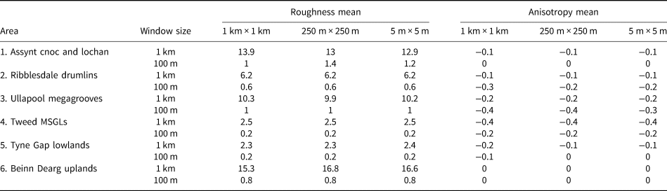
The means were calculated by combining values for both flow directions. In addition to the mean bed roughness and anisotropy for a 5 m × 5 m resolution grid reported in Table 2, we report values for 1 km × 1 km and 250 m × 250 m resolution grids.
Conclusions
The groups of glacial landforms investigated here have a characteristic bed-roughness signature when bed-roughness anisotropy is taken into account. Anisotropy is key to defining the bed-roughness signatures of glacial landforms assemblages because this allows landforms with similar roughness values to be differentiated, e.g. cnoc and lochan and megagrooves (areas 1 and 3). This is the first study to show that glacial landforms have a characteristic bed-roughness signature, and this information could be used to infer the nature of landforms at the bed and where they are located underneath contemporary ice streams.
The results showed that a window size of 100 m was more appropriate for mesoscale and some macroscale landforms, whereas a window size of 1 km was better suited to macroscale landforms that were wider than 100 m and had a large spacing. However, both window sizes are required to determine the characteristic bed-roughness signatures of a wide range of landform types. It must be noted that to facilitate comparison between studies, window sizes must be the same. We suggest that this roughness-signature method needs to be further tested on other deglaciated areas before it can be used to identify landforms on contemporary-ice-sheet beds.
There are many unanswered questions about the environment at the bed of ice streams, such as how are landforms created, and what processes are involved in their growth over time? How do changes in landform dimensions affect bed roughness, and consequently affect ice velocity? There are certain feedback loops that occur. The geomorphology of the bed influences ice velocity e.g. a rough bed causes slow speeds, but ice flow can smooth the shape of the bed and thus increase in speed. Finding out more information about this feedback loop is important because it could be key in our understanding of ice-stream beds. We have demonstrated that bed-roughness measurements with anisotropy data can be used to start to answer some of these questions.
Acknowledgements
This paper is dedicated to Nilo Falcini, who had a great scientific mind and a keen interest in understanding the Earth. Many thanks to Jon Hill and Colin McClean from the Environment and Geography Department at the University of York, who provided advice and guidance on the methods used. We thank the sub-editor and editor (Iestyn Barr and Hester Jiskoot) and two reviewers (Jeremy Ely and one anonymous reviewer) for their helpful and insightful comments, which significantly improved this paper. This research is part of a Ph.D. project, funded by NERC, grant number NE/K00987/1. OS Meridian data were provided by the Ordnance Survey, Crown copyright and database right 2012. NEXTMap DTM was provided by NERC via the Centre for Environmental Data Analysis (CEDA).


 Open access