


1. Introduction
The Global Navigation Satellite System (GNSS) can provide position, velocity and timing (PVT) information. GNSS-based positioning and navigation consist of different time scales for receiver and satellites; both time scales are synchronised by linking them to GNSS time. The satellite clock biases in the observation equation are accounted from the broadcast navigation message or by using orbit and clock products of the International GNSS service (IGS, Dow et al., Reference Dow, Neilan and Rizos2009). On the other hand, the receiver clock biases in the observation equation must be estimated at every epoch due to the poor long-term frequency stability of the internal quartz oscillator within the receivers. With three coordinates and a receiver clock bias, there are four unknowns to be estimated at each epoch. This leads to a weakened observation geometry and the requirement of a minimum of four satellites to obtain a solution (Bednarz and Misra, Reference Bednarz and Misra2006). In addition, the estimated clock time bias, up coordinate and tropospheric delay are highly correlated (Rothacher and Beutler, Reference Rothacher and Beutler1998; Santerre et al., Reference Santerre, Geiger and Banville2017). Also, the up coordinate is estimated less precisely than is the horizontal coordinate. All of these drawbacks can be greatly improved if an oscillator with higher frequency stability is used to drive the internal circuitry of the receiver; consequently, knowledge about the frequency stability of the oscillator is used during the estimation process (Sturza, Reference Sturza1983; Weinbach and Schön, Reference Weinbach and Schön2011). This technique is referred to as receiver clock modelling (RCM), sometimes also known as clock coasting.
For kinematic applications, positioning can be computed with just three satellites at each epoch with clock coasting (Sturza, Reference Sturza1983; Knable and Kalafus, Reference Knable and Kalafus1984; Krawinkel and Schön, Reference Krawinkel and Schön2015). In RCM, the receiver clock is modelled with a linear polynomial over certain time spans, which allows avoidance of an epoch-wise estimation of the clock time bias. It also strengthens the observation geometry and the positioning results are more robust. Results from a kinematic experiment in an open-sky environment shows that the precision of the up coordinate is improved by about 50–70% when RCM is applied; the reliability of the system is amplified further, leading to a more robust position estimation (Krawinkel and Schön, Reference Krawinkel and Schön2016). The impact of RCM is also studied with a real flight experiment comprised of extremely dynamic manoeuvres; results demonstrate a significant gain in the overall system's performance (Jain and Schön, Reference Jain and Schön2020).
Positioning and navigation requirements vary with the application type, i.e. in safety critical services, accuracy, precision, continuity and availability needs are quite strict, whereas in pedestrian navigation, there is a certain degree of leverage available with the parameters. GNSS navigation in urban surrounding is severely impacted by signal degradation. This degradation mainly arises due to signal blockages from tall buildings, reception of non-line-of-sight (NLOS) signals, multipath and diffraction effects etc. To encounter the mentioned issues in urban areas, aided navigation techniques are being utilised. For example, GNSS receivers are being coupled with inertial measurement units (IMU) to encounter for phases where in GNSS signals are completely blocked. Due to the widespread availability of three-dimensional (3D) city models, GNSS can be used to detect line-of-sight (LOS) and NLOS signals from satellites in urban areas and improve the positioning accuracy (Bradbury et al., Reference Bradbury, Ziebart, Cross, Boulton and Read2007; Hsu et al., Reference Hsu, Gu and Kamijo2015; Icking et al., Reference Icking, Kersten and Schön2020). The 3D city models can also be used with shadow matching to enhance GNSS positioning in urban areas (Groves, Reference Groves2011; Wang et al., Reference Wang, Groves and Ziebart2013). Although all the aided navigation techniques are efficient, they are computationally expensive, thereby acting as hindrances in various applications.
Positioning performance of several mass-market receivers in open-sky, rural, semi-urban and urban environments is explained (Štern and Kos, Reference Štern and Kos2018). The paper concludes that to achieve sub-meter accuracy, a hybrid multisensor approach is necessary with mass-market receivers. Multiple challenges that future automotive GNSS positioning could face in urban areas are listed; performance improvement with multi-GNSS dataset is shown (Escher et al., Reference Escher, Stanisak and Bestmann2016). The use of data gathered in an urban surrounding with software-defined radio (SDR) technology allows improvement to the system's performance (Cristodaro et al., Reference Cristodaro, Dovis, Falco and Pini2017). However, the processing load is higher and there is a considerable latency to obtain the solution. Low-cost high-sensitivity (HS) GNSS receivers are capable of tracking signals with very low carrier-to-noise density ratios (C/N0) in comparison with the geodetic grade GNSS receivers. However, the noise levels of the signals recorded by HS receivers could be higher in comparison with the geodetic receiver due to their limited hardware. As with RCM, the height coordinate can be estimated more precisely and it can be used in faster tracking of people during emergency situations in urban setups. Also, it can lead to a better user experience for an application dependent on height parameters. Due to the excellent signal-tracking capabilities of HS receivers and capability achieved with RCM to maintain availability and continuity in challenging conditions, the performance an HS receiver with an external clock in an urban surrounding must be assessed.
This paper addresses the feasibility of using a standalone HS multi-GNSS single-frequency receiver with external clock on a mobile platform in an urban environment. The performance gain in positioning and navigation is evaluated and compared for two different receiver types (i.e. HS and geodetic-grade) with RCM. Both the receiver types were driven with the same external atomic clock, namely a Microsemi miniaturised atomic clock (MAC) SA.35 m (Microsemi, 2019). To the best of our knowledge, it is the first instance of RCM applied in an urban kinematic experiment with a standalone low-cost HS receiver. First, the concept of RCM in code-based GNSS navigation is described. In addition, the linearised Kalman filter (LKF) algorithm used for state estimation with and without RCM is detailed. Later, the measurement setup and kinematic experimental campaign carried out to record GNSS observations in an urban environment is thoroughly explained. The recorded observations with different receiver types are then investigated by comparison in terms of different parameters, such as number of recorded observations, code, and Doppler noise and received signal strengths with regards to different segments of the experiment. The position and velocity estimates computed with and without RCM using a LKF approach are discussed and the performance improvement is quantified. The impact of the different receiver types on the navigation performance is highlighted. Finally, conclusions are drawn based on the performance of the HS and geodetic receivers in the urban scenario.
2. Receiver clock modelling and Kalman filtering
2.1 Principle of RCM
The process wherein the internal temperature compensated crystal oscillator (TCXO) of the GNSS receiver is replaced with an external oscillator possessing high frequency stability allows modelling its operation in a physically meaningful way over a certain time duration. This method is referred as RCM and it further strengthens the observation geometry over the modelling time duration. In RCM, it is mandatory that the oscillator noise is less than the GNSS receiver noise. Thus, the random integrated frequency fluctuations of the oscillator cannot be resolved by the GNSS observations (code, phase or Doppler).
Oscillator characterisation is typically done based on time-dependent Allan variance $({{\sigma_y}^2} )$ parameter (Allan, Reference Allan1987). This measure allows determining the time prediction errors, which in turn enables to find the time modelling duration over which RCM holds true, i.e. oscillator noise is less than the GNSS receiver noise. Furthermore, the RCM time duration can also be computed based on the power spectral density of the signal (Allan et al., Reference Allan, Hellwig, Kartaschoff, Vanier, Vig, Winkler and Yannoni1988). The noise of the GNSS receiver can be assumed to be about 1% of the signal wavelength in use, i.e. 3 m for L1 C/A code, 0⋅002 m for L1 carrier phase observation. For L1 Doppler observation, the noise can be assumed to be about 0⋅05 m/s.
In the kinematic experiment, a Microsemi MAC SA.35 m oscillator is used. It is a rubidium (Rb) standard atomic clock and its frequency signal serves as clock input to a geodetic grade JAVAD Delta GNSS receiver and a HS low-cost u-blox receiver. To validate the frequency stability information provided in the manufacturer's datasheet and compute the appropriate RCM time duration, a clock characterisation study is carried out in a laboratory at PTB – The National Metrology Institute of Germany, in terms of the short- and long-term frequency stabilities. From this study, it is observed that the estimated frequency stability of MAC SA.35 m agrees with the manufacturer's values. Moreover, the performance of the oscillator is also evaluated in a highly dynamic environment and all the results are shown in Jain et al. (Reference Jain, Krawinkel, Schön and Bauch2020).
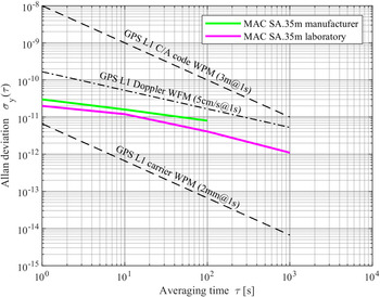
The Allan deviation (ADEV) values obtained from the MAC SA.35 m manufacturer's datasheet and computed from laboratory dataset for averaging time from one second to about 17 min are shown Figure 1. In addition, ADEV's for GPS L1 C/A code, phase and Doppler observations for the same averaging time are depicted in Figure 1. As code and carrier-phase observations are phase-based measurements, the noise of C/A code and phase observations are modelled as white phase modulation (WPM) over time, whereas the noise of Doppler is modelled as white frequency modulation (WFM) over time. As shown in Figure 1, the noise of MAC SA.35 m is smaller than the noise of GPS L1 C/A code and Doppler observations but higher than the carrier phase observations. Hence, RCM cannot be applied with phase observations using this oscillator. The estimated ADEV's from laboratory dataset for MAC SA.35 m are transformed to spectral density ${h_\alpha }$ coefficient (Barnes et al., Reference Barnes, Chi, Cutler, Healey, Leeson, McGunigal, Mullen, Smith, Sydnor, Vessot and Winkler1971). Using this ${h_\alpha }$
 coefficients specified in Jain et al. (Reference Jain, Krawinkel, Schön and Bauch2020), the spectral behaviour of the oscillator can be modelled through the process noise matrix when estimating state parameters (e.g. position, velocity and timing) through a Kalman filtering approach.

Figure 1. ADEV of microsemi MAC SA.35 m from manufacturer's datasheet and derived from characterization carried out in a laboratory at PTB. GPS L1 C/A code and L1 carrier phase observation noise modelled as white phase modulation (WPM); GPS L1 Doppler noise modelled as white frequency modulation (WFM)
2.2 Kalman filter estimation
In the case of GNSS-based PVT solution, different state errors are estimated largely using a LKF. Moreover, this technique is used in variety of other applications due to its performance, computational efficiency and applicability in real time. It is the best possible linear-estimator with minimum variance when optimum values for measurement and process noise are known (Brown and Hwang, Reference Brown and Hwang2012). In comparison with state estimation with least-square adjustment (LSA), Kalman filter integrates system dynamics along with appropriate process noise models. Different motion models could be used to account for dynamics. During phases when the motion model becomes invalid, the filter can be tuned with process noise up to a certain limit, i.e. uncertainty in the states can be bounded.
The observation equation for pseudo-range measurements in GNSS-based navigation solution between a receiver A and satellite i is

where $X,\; Y$ and Z = respective geocentric coordinates for the receiver A and satellite i; $T_A^i$
 and $I_A^i$
 = tropospheric and ionospheric signal delays; c = speed of light; $\delta {t_A}$
 and $\delta {t^i}$
 = respective receiver and satellite clock errors; $\delta t_{A,\; rel}^i$
 = relativistic time offset and $\epsilon _A^i$
 = measurement noise. The ionospheric and tropospheric (wet and dry components) delays are accounted using IGS ionospheric exchange total electron content (IONEX TEC) map (Schaer et al., Reference Schaer, Gurtner and Feltens1998) and the Vienna mapping function 3 (Landskron and Böhm, Reference Landskron and Böhm2018), respectively. In addition, the satellite clock errors and relativistic time offsets are corrected by the orbit and clock products from the multi-GNSS experiment (MGEX) of IGS (Montenbruck et al., Reference Montenbruck, Steigenberger, Prange, Deng, Zhao, Perosanz, Romero, Noll, Stürze, Weber, Schmid, MacLeod and Schaer2017). $\bar{l}_k^i$
 is computed for every visible satellite along the complete time series of the dataset. Correspondingly, by using the observation equation for Doppler measurements and appropriate modelling, Doppler observations are computed. Finally, computed code and Doppler observations form the observation vector ${\bar{\textbf{l}}_k}$
 .
.
Due to the nonlinear relation between the recorded observations ${\textbf{l}_k}$ and state vector ${\textbf{x}_k}$
 , the observed-minus-computed (OMC) vector $\Delta {\textbf{l}_k}$
 is formed, i.e. the difference between the recorded code and Doppler observations ${\textbf{l}_k}$
 and computed observations ${\bar{\textbf{l}}_k}$
 . With a LKF, the error state vector $\Delta {\hat{\textbf{x}}_k}$
 is computed and then added to the a priori state ${\bar{\textbf{x}}_k}$
 to obtain the final estimate state ${\hat{\textbf{x}}_k}.$
For the initialisation epoch, the error state and its corresponding variance–covariance matrix (VCM) are set as

Apart from the initialisation step, the error state vector and its VCM are filtered in the update step:

with the design matrix ${\textbf{A}_k}$ containing the partial derivatives of the functional model evaluated at the nominal trajectory. The observation uncertainty ${\textbf{Q}_{ll,k}}$
 is derived using SIGMA- variance model. It was first proposed by Hartinger and Brunner (Reference Hartinger and Brunner1999) for GPS carrier phase observations and is given as

where $C/{N_0}$ = measured carrier to noise density ratio of the signal in dB-Hz, and ${C_v}$
 = variance factor dependent on the receiver–antenna configuration and is estimated from the transformed samples. The applicability of the SIGMA- variance model was further extended and proven with GPS code observations; an improvement in position accuracy was shown to be about 30–50% using real urban data recorded with different types of HS receivers (Wieser et al., Reference Wieser, Gaggl and Hartinger2005). Overall, the model is based on variance factors that are pre-derived for each specific receiver–antenna combination and different GNSS systems based on recorded $C/{N_0}$
 of corresponding signals in an open-sky static environment. It must be noted that these calibrated variance factors are not specific to any surrounding in regards to its utilisation.
To compute the variance factors for both code and Doppler observations, a static study is carried out with exactly the same measurement setup. For multiple receivers of the same type, the variance factors obtained after post-processing the static dataset are almost similar considering the respective GNSS system. Hence, its mean value is computed and listed in Table 1 for the code observations. For the Doppler observation variance factors, the reader is referred to Jain et al. (Reference Jain, Kulemann and Schön2021). These variance factors are then used to model the variance of the corresponding pseudo-range and Doppler observations in relation to the measured $C/{N_0}$ during the kinematic experiment.
Table 1. Estimated code observation variance factors for different receiver-antenna combinations

The Kalman gain ${\textbf{K}_k}$ is evaluated as

Later, the prediction step is performed where the updated error states are time propagated:

where ${\mathbf{\Phi }_{\boldsymbol{k}}}$ = transition matrix and ${\textbf{Q}_{\omega\omega,k}}$
 = process noise matrix. For the kinematic dataset processing, the transition matrix is selected based on a constant velocity (CV) model. The process noise for the corresponding position and velocity states are modelled as a random ramp and a random walk process, respectively. In the case of RCM, the elements of clock process noise matrix (${\textbf{Q}_{ \omega\omega- \textrm{clk},k}}$
 ) are computed using the spectral density ${h_\alpha }$
 coefficients of the oscillator in use and is given as

where ${h_0} = 8 \times {10^{ - 22}},\; \; {h_{ - 1}} = 7 \cdot 2 \times {10^{ - 25}}$ and ${h_{ - 2}} = 3 \times {10^{ - 29}}$
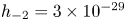 are the spectral density coefficients of white frequency noise (WFN), flicker frequency noise (FFN) and random-walk frequency noise (RWFN) applied in this study, respectively. More information about the computation of the process noise matrix in the absence of RWFN spectral coefficient and its implementation in KF is explained by Krawinkel (Reference Krawinkel2018). For the case when RCM is not applied, the clock time offset is modelled as a random ramp process, whereas the clock frequency offset is modelled as a random walk process. It must be noted that different results of the KF with and without applying RCM are exclusively due to the differences in the clock process noise models.
3. Urban area experiment
To verify the operational feasibility of the HS u-blox receiver driven with an external atomic clock (i.e. u-blox 1771 driven with MAC SA.35 m in our case) in kinematic mode, a measurement is performed in urban areas. Moreover, the performance gain in the positioning domain is also evaluated by applying the concept of RCM with different receiver types.
3.1 Experiment measurement setup
The measurement configuration and the vehicle used during the experiment is shown in Figures 2(a) and 2(b), respectively. It consists of two geodetic-grade JAVAD GNSS receivers [type: Delta TRE-G3 T(H)], and two HS u-blox receivers (type: NEO M8 T). Both JAVAD GNSS receivers were running on the same firmware version, and the same applies for the u-blox receivers. In addition to the four receivers, there was a Microsemi miniaturised atomic clock (MAC) SA.35 m, a Novatel SPAN receiver connected with iMAR inertial measurement unit (IMU) and an active GNSS splitter, which was connected to the geodetic antenna (type: JAVAD GrAnt G3 T) placed at the top of the vehicle.

Figure 2. Kinematic experiment in hannover. (a) measurement setup, (b) institute vehicle used during the experiment
The internal circuitry of JAVAD receiver (0082) and u-blox receiver (1771) were driven by MAC SA.35 m, whereas the other JAVAD receiver (0081) and u-blox receiver (0867) were not modified and were driven by their own internal TCXO. For the u-blox receiver (1771), there is no external frequency input as for the JAVAD receivers, which makes connecting an external clock straightforward. The TCXO within u-blox (1771) was removed; the 10 MHz signal from the MAC SA.35 m was modulated with a signal wave generator (SWG) to 26 MHz (i.e. u-blox clock signal frequency) and fed via a connector to the receiver. The feasibility and PVT performance of this modified u-blox receiver (1771) in an open-sky static environment is explained by Bochkati and Schön (Reference Bochkati and Schön2018). The Novatel SPAN receiver in conjunction with the iMAR IMU forms a multisensor system and records IMU data in GPS time frame. From this IMU data, GNSS data from a reference station located at our institute laboratory terrace and GNSS data from JAVAD receiver (0082), a tightly coupled (TC) reference trajectory solution was computed for the complete duration of the urban experiment. It must be noted that the computation is done in relative carrier phase-based GNSS post-processing mode using the TerraPos software (Kjørsvik et al., Reference Kjørsvik, Øvstedal, Gjevestad and Sideris2009).
3.2 Test drive details
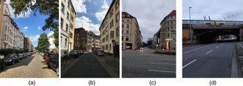
The kinematic experiment was carried out on 22 May 2019 around the western and southern part of the city of Hannover, Germany. The experiment lasted for a duration of about two hours and the complete test route is shown in Figure 3. The test route is comprised of a variety of light and moderate urban conditions, ranging from open-sky to overhanging trees and branches, to narrow roads surrounded by buildings of heights in the range of about 20–30 meters on both sides. Such conditions lead to multipath, blockage or attenuation of signals and interference with other high-intensity signals from the adjacent GNSS frequency bands. The measurement starts with a static phase of about seven minutes in a parking area; later, the vehicle starts moving. It first passes through the inner-city area, which has a more open-sky characteristic. Following this, the vehicle moves along Marienstraße, where the street is mostly flanked on both sides by buildings (Figure 4c). Later, a certain loop, shown in right part of Figure 3, was driven six times, with the first loop being slightly larger and its beginning is marked with point B. The following five loops were exactly similar, taking approximately seven minutes per loop and its ending is marked with point C. Some pictures of the streets along the loop route are shown in Figures 4(a) and 4(b). It consists of mostly three-storey buildings on both sides with some tress and very narrow streets, with the width being in the range of about 4-6 m. Later, another test loop is driven more than two times and its start is marked with point D in Figure 3. This loop route includes Marienstraße, two underpasses and an overhead bridge. Figure 4(d) is an example street view picture of one such underpass. Moreover, there are several standstill phases at traffic signals and crossings along the complete test route. The details of the marked points on the urban trajectory map and their approximate GPS times are listed in Table 2.

Figure 3. Full measurement drive route (left); zoomed in loop route driven during the experiment (right). For details of the marked points with ‘×’, cf. Table 1. The other labels in round brackets denotes different paths along the experiment and are shown in next figure. The arrow indicates direction of travel during the experiment. Underlying map presentation taken from google maps

Figure 4. Images of different streets through which the kinematic experiment is conducted. Street view of simrockstraße (a), große barlinge (b), marienstraße (c) and schiffgraben (d). All the streets shown lie in the southern part of hannover and are indicated in Figure 3 with same corresponding labels
Table 2. Summary of marked points on the map

Each receiver was recording GPS, GLONASS and Galileo pseudo-range, carrier phase and Doppler observations and their corresponding signal strength. The sampling rate was set to 1 Hz for all the receivers and an elevation cut-off angle was not applied while recording the data. The geodetic-grade JAVAD GNSS receivers used in the experiment have the capability to track multiple frequencies (L1, L2 and L5) simultaneously, while the HS u-blox receivers can only track the L1 frequency of each GNSS system.
4. Results
First, measurement data recorded with receivers (JAVAD 0082 and u-blox 1771) connected with MAC SA.35 m are analysed in terms of their quality and statistics. Secondly, the navigation performance is evaluated with RCM in regards to the different segments of the urban experiment. Analysis of data recorded with other receivers driven with internal TCXO are not included for the sake of conciseness, except for one case which shows results of RCM applied when it is physically not meaningful.
4.1 Measurement data analysis
The zero-baseline configuration between the JAVAD 0082 and u-blox 1771 receiver allows us to compare the signal quality of different receiver grades and gauge their performance on a mobile-platform in urban environment. The measurement data analyses are limited to L1 frequency signals of different GNSS systems, as u-blox HS are only capable of tracking them. A detailed analysis of the carrier-phase observations recorded during the experiment with all the receivers and its characteristics with respect to the different weighting models is explained in Ruwisch et al. (Reference Ruwisch, Jain and Schön2020).
4.1.1 GNSS signal statistics
The aggregate number of code and phase observations recorded during the test drive from L1 frequency GPS, GLONASS and Galileo signals are listed in Table 3. In addition, the exact receiver independent exchange (RINEX) format specifier for the recorded observation type is also mentioned. The number of recorded corresponding Doppler observations is exactly equal to code observations for both the receivers. The recorded number of GPS observations are the highest, followed by GLONASS and Galileo for both receiver types. As expected, the number of recorded code observations from all GNSS are considerably higher with the u-blox 1771 in comparison with the JAVAD 0082 receiver. The number of recorded phase observations is equal to the code observations with the JAVAD 0082 receiver. However, the u-blox 1771 receiver is recording about 20% to 25% fewer phase observations compared with the code. For application requiring higher accuracy and precision, phase observations are preferred and, hence, it is a limiting factor for the HS-type receiver.
Table 3. Total number of L1 code and phase observations recorded from different GNSS during the urban experiment

4.1.2 Signal strength analysis
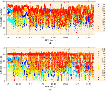
Figures 5(a) and 5(b) show the measured C/N0 of GPS L1 C/A code observations from all the tracked satellites by Javad 0082 and u-blox 1771, respectively. Both receivers were connected with a Microsemi MAC SA.35 m oscillator. The vertical black dashed lines in Figure 5 and all the following figures correspond to the different marked points in the urban experiment map depicted in Figure 3. The u-blox 1771 receiver tracks two more satellites than the JAVAD 0082, albeit only for very few epochs. With the JAVAD 0082 receiver, the values of the measured C/N0 lies mostly in the range of about 20 to 55 dB-Hz. On the other hand, for the u-blox 1771 receiver, they mostly lie in the range of about 15 to 52 dB-Hz. During the repeatedly driven route (i.e. segment B–C), many observations are recorded with a lower C/N0 in comparison with other segments with the JAVAD 0082 receiver. This reduction in the measured C/N0 is mainly due to an environment consisting of tall buildings and trees leading, to multipath and diffraction effects along the corresponding route. On the contrary, with the u-blox 1771 receiver, there is no significant change in the measured C/N0 with regards to the different segments. Also, the number of observations measured with lower C/N0 (i.e. between 10-25 dB-Hz) is very high in segment B–C with the u-blox 1771 compared with the JAVAD 0082 receiver, thereby validating the capability of tracking weak signals with HS-type receivers. The variation in the measured C/N0 from different satellites is visible in both the receivers and it is due to the different satellite elevation angles. Towards the end of segment A–B where the car was static for a few minutes, the varying C/N0 from different satellites measured on both the receivers reveal almost an identical behaviour.

Figure 5. C/N0 of GPS L1 C/A code observation recorded from different satellites on JAVAD 0082 (a) and u-blox 1771 (b) receivers in relation with the GPS time of the urban experiment. Satellites are colour coded
4.1.3 Quality of recorded code observations
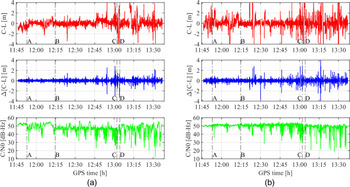
For zero-baseline measurements, the code-minus-phase (C-L) range can be used to evaluate the code noise (De Bakker et al., Reference De Bakker, Van Der Marel and Tiberius2009). The phase noise and multipath value is at least one order magnitude less than the code noise and multipath component; hence, it can be neglected. The results of C-L consist of twice the residual ionospheric error, multipath error and ambiguities from the phase range if they are not accounted. In our processing, we used the OMCs of code and phase ranges, thereby reducing the ionospheric errors up to a large extent. Further, the ambiguities are also accounted and the results obtained for GPS PRN29 recorded on JAVAD 0082 and u-blox 1771 are shown in the top pane of Figure 6. Data from satellite PRN29 is selected, as it is available during the whole experiment duration. The oscillating behaviour seen in both top panes towards the end of the segment A–B is mostly probably caused due to multipath. Interestingly, the C/N0 depicted in the bottom pane of Figure 6 shows almost negligible variation for the corresponding part. During the last segment (D–end) of the experiment, the deviations in code noise is larger compared with the other segments for both receivers. In addition, the corresponding measured C/N0 has larger variations. It is mainly due to experiment condition in the last segment resulting in large multipath errors, signal blockage, attenuation etc. The standard deviation of the code noise computed with C-L along the complete trajectory is about 0⋅75 m and 1⋅6 m for the JAVAD 0082 and u-blox 1771 receiver, respectively.

Figure 6. L1 code noise along the complete trajectory for GPS PRN29 recorded with JAVAD 0082 (a) and u-blox 1771 (b) receivers, respectively. In both plots, the top subplot depicts code-minus-phase un-differenced case, middle is the time differenced case while the bottom is the corresponding C/N0 measured with the respective receivers
To reduce the multipath errors and remove the ambiguities completely, the time-differenced code-minus-phase (Δ[C-L]) range can be computed. The undifferenced C-L results shown in both top panes of Figure 6 are time-differenced and presented in the middle panes. It is seen that the multipath errors are almost removed with data from both receivers. Most of the peaks visible and larger variations that can be seen in the Δ[C-L] corresponds to lower C/N0 values. Finally, the standard deviation of the code noise computed with Δ[C-L] along the complete urban track is about 0⋅24 m and 0⋅35 m for the JAVAD 0082 and u-blox 1771 receiver, respectively. The higher code noise with the HS-grade receiver is due to the limited hardware. In general, with data recorded from all other GNSS satellites, it is seen that the noise level is higher with lower C/N0 values, which in turn also depends on the elevation angles of the satellites.
4.1.4 Analysis of Doppler observation
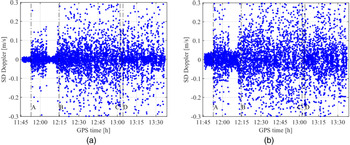
Figures 7(a) and 7(b) depict the single differences (SD) among GPS L1 C/A Doppler observations recorded on the JAVAD 0082 and u-blox 1771 receivers, respectively, from satellite PRN29 and PRN31. As per the principle of ‘between-satellite’ SD involving code and phase ranges from a satellite, the receiver clock error cancels out. When this concept of between-satellite SD is extended to Doppler observations, the receiver clock frequency offset is removed. In addition, we use the Doppler OMCs to compute the noise levels. The advantage of using Doppler OMCs is that all the possible errors (satellite and relativistic frequency offsets, tropospheric and ionospheric delay rate) that could affect the observations are already modelled and accounted. As expected, the phases wherein the vehicle is static during the experiment (i.e. initial phase, at traffic signals and crossovers), the noise level is significantly lower compared with the phase where the vehicle is in motion. To be specific, the noise level during the static phases is about ±1⋅5 cm/s with the JAVAD 0082, whereas it rises to about ±3⋅5 cm/s with the u-blox 1771 receiver. From segment encompassing from point B until the end of the experiment, the noise level spread is largely varying, and it is mainly due to overall signal reception conditions. The standard deviation of the noise level after ignoring outliers with the JAVAD 0082 and u-blox 1771 receiver along the complete experiment time series is about 25 cm/s and 55 cm/s, respectively. This significant difference in the noise levels between the receiver types could be a quality indicator in terms of the precision that could be achieved. Also, the considerable difference between the noise levels in static and moving phases must be accounted properly with adequate variances of the Doppler observation during velocity estimation.

Figure 7. Single differences between GPS L1 Doppler observations recorded from PRN29 and PRN31 on JAVAD 0082 (a) and u-blox 1771 (b) receivers. Note that the y-axis scale is bounded with certain limits for better pictorial representation
4.2 Position and velocity estimation analysis
The receiver PVT states are estimated based on the LKF algorithm explained in section 3. The results are obtained with and without applying the concept of RCM. All the observations received from satellites with an elevation angle of less than 10° are neglected during the estimation process. Also, outliers are identified based on a local slippage (LS) test (Teunissen, Reference Teunissen1990). Once an outlier is identified, the corresponding observation is down-weighted. The parameters are re-estimated and the test is performed again. A single observation is down-weighted by a factor of 10 for up to five times before rejecting the observation for that specific epoch. The adaptation of the observations is done considering the urban environment where typically the observation count is scarce.
When the stability of an atomic clock is introduced in the process noise matrix when dealing with datasets of receiver driven by its own internal TCXO, it is not valid. To illustrate this effect of applying RCM when it is physically not meaningful, the dataset recorded on the JAVAD 0081 was used. Figure 8 shows topocentric coordinate and velocity differences w.r.t the reference trajectory and the clock time/frequency offsets evaluated with and without RCM for JAVAD 0081. The coordinate deviations after ignoring a few large spikes along the horizontal and vertical components is as expected and about 1 m and 3 m, respectively, when RCM is not applied. With RCM, a drift is observed in the estimated coordinates in the segment B–C and it reflects the poor long-term frequency stability of the internal TCXO. The velocity deviations along the horizontal and vertical component are seen scattered around zero mean for the computation without RCM. Also as expected, the variation in the estimated velocities during static phases is quite small when compared with the dynamic phases of the experiment. The velocities estimated with RCM depicts a drift, with it being more pronounced in the vertical component when compared with the horizontal. A significant drift is also visible in the estimated clock-frequency offsets with and without RCM; however, the drift seen is much smoother when computed with RCM. Also, the receiver-clock offsets estimated after a straight-line fit is almost the same (effect of integration of the respective frequency offsets) with and without RCM; it does not happen when RCM is applied in true sense (cf. Figure 9 and Figure 10). Thus, one cannot just use better clock stability characteristics to process the datasets and improve systems accuracy, precision and overall robustness.
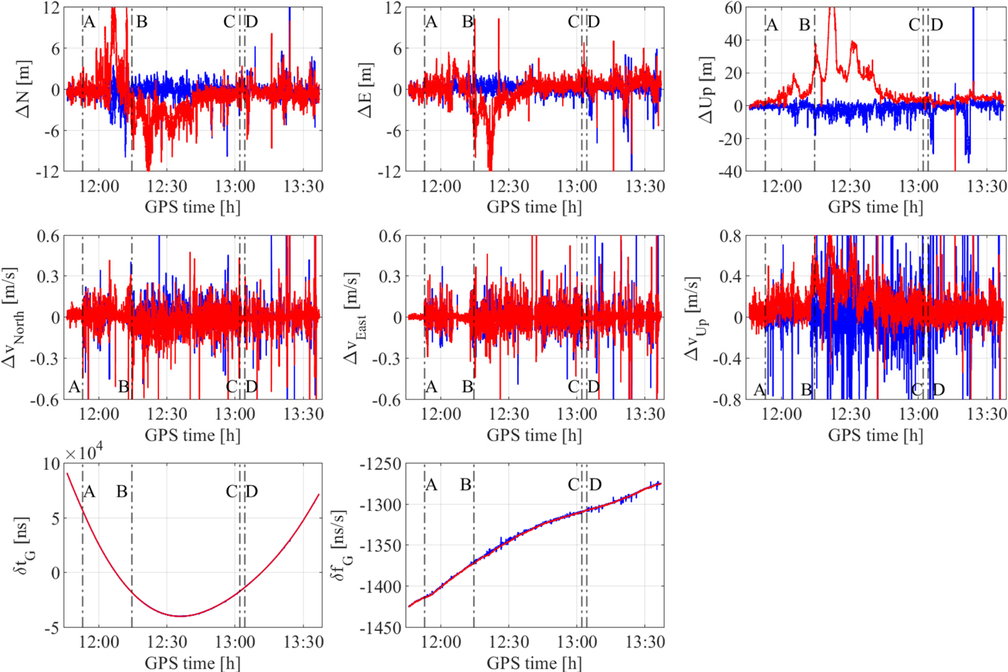
Figure 8. Topocentric coordinate and velocity deviation relative to the nominal trajectory and clock time/frequency offsets evaluated with (red) and without (blue) RCM for JAVAD 0081 receiver. The clock time offset is linearly detrended

Figure 9. Topocentric coordinate and velocity deviations relative to the nominal trajectory and clock time/frequency offsets computed with (red) and without (blue) RCM for JAVAD 0082 receiver, connected to MAC SA.35 m. The clock time offset is linearly detrended
Figure 10. Topocentric coordinate and velocity deviations relative to the nominal trajectory and clock time/frequency offsets evaluated with (red) and without (blue) RCM for u-blox 1771 receiver which is connected to MAC SA.35 m. The clock time offset is linearly detrended
The topocentric coordinate and velocity deviations computed with and without RCM for data recorded on the JAVAD 0082 and u-blox 1771 receivers are shown in Figure 9 and Figure 10, respectively. In addition, receiver-clock time and frequency offsets evaluated for both receivers with and without RCM are also depicted in different colours, respectively. The solution is computed using unsmoothed GPS, GLONASS and Galileo code and Doppler observations. For the JAVAD 0082 and u-blox 1771, the residual noise along the north component for segment (A–end) is about 1 m and 2 m, respectively, without applying RCM. These residual values are almost similar even when RCM is applied. Some large spikes are visible, specifically towards the end of segment A–B and segment D–end; all of them could be attributed to poor observation geometry and noisier observations due to multipath effects. The deviations of the velocity component in the north direction along the complete time series is about 8 cm/s and 21 cm/s for JAVAD 0082 and u-blox 1771, respectively, with and without applying RCM. The noise levels along the east coordinate and velocity component are comparatively less than the north for both the receivers. Also as expected, there is no additional gain in terms of reduction in the noise level when RCM is applied. During the static phases of the experiment (e.g. Start–A), the coordinate and velocity deviations along all directions is significantly smaller compared to the values obtained in other segments (e.g. B–C, D–end).
There is a distinct improvement in the precision of the up component when RCM is applied with both the receivers. The precision improvement is 73% for the JAVAD 0082 and 68% for the u-blox 1771 receiver. Similarly, for the velocity up component, the gain is significant in terms of precision and is 68% and 72% for JAVAD 0082 and u-blox 1771, respectively. It is worth noting that all the spikes seen in segment A–end when RCM is not applied are drastically reduced in the up component when RCM is applied. Hence, it can be said that solution is more robust when RCM is applied. In terms of accuracy, there is an improvement of at least 48% and 62% in the up coordinate and velocity components with both receivers when RCM is applied. The standard deviation of the topocentric errors for different segments of the experiment evaluated for both receivers are listed in Table 4; the up-coordinate and velocity-component precision is improved in all the kinematic segments.
Table 4. Standard deviations of position and velocity deviations in the topocentric frame for different segments of the experiment for both receivers

As both receivers are operating in a common-clock configuration, the time and frequency offsets are expected to be similar. The receiver clock offsets (i.e. linear detrended) and frequency offsets values lie in the range of about ±100 ns and ±10 ns/s for both the receivers, respectively. These values reflect the high-frequency stability of the MAC SA.35 m external oscillator and verifies the common-clock mode. Moreover, the estimated clock time and frequency offsets for both receivers are reduced drastically when RCM is applied. A significant difference is observed with the noise level when compared in terms of the different receivers. This is because during state estimation, the number of satellites and the corresponding observation quality used for processing is different for both the receivers. In particular, for JAVAD 0082, the clock time and frequency offsets seem to be smooth in comparison to for u-blox 1771, where the clock offsets are jittery. All the corresponding deviations visible in the clock time offsets for both receivers translate into spikes in the up component, indicating high correlation among clock time offset and the up component. With RCM, the up component and velocity with RCM for JAVAD 0082 is bounded quite well and it is mainly due to the fact that for RCM to be physically meaningful, the clock noise must be less than the GNSS observation noise. In the case of u-blox 1771, the results for up component and vertical velocity with RCM are also valid but contained some additional spikes; this was due to the observations being processed from different satellites, in comparison with the JAVAD 0082 receiver. Overall, the results validate the importance of applying RCM only when it is physically meaningful and an external oscillator is used with a high-sensitivity grade receiver in an urban mobile platform.
On further investigation, it was found that the large spikes obtained without applying RCM (one towards end of segment A–B and some in segment D–end) corresponds to the vehicle moving or being static along the Marienstraße [Figure 4(c)]. Due to the surrounding environment, it can be said that most of the signals recorded during this time were reflected or diffracted from buildings on both sides of the street. These multipath errors can be reduced largely by considering a 3D city model or shadow matching, as stated earlier.
In terms of availability, a solution was always possible with the u-blox 1771 receiver, whereas it was missing for 39 epochs with the JAVAD 0082 receiver. Out of these 39 epochs, there were 8 epochs where no data was recorded as the vehicle crossed multiple underpasses in the city. For other cases, there were not enough observations to compute a solution. Table 5 provides the number of code and Doppler GNSS observations used during processing and the corresponding number of detected outliers with and without applying RCM. The number of code and Doppler observations used during the processing are same. The count of GNSS observations used for processing differs from the values presented in Table 3 as an elevation mask of 10° is applied. As the data is recorded in a challenging environment, the biases in the observations are higher and, hence, the number of detected outliers are quite large. The percentage of code and Doppler outliers detected with respect to the total corresponding GNSS observations used during processing with the JAVAD 0082 are comparatively smaller than with the u-blox 1771. For both the receivers, Doppler observation are much more sensitive to outliers than code observations. With the u-blox 1771, the percentage of different GNSS Doppler outliers with and without applying RCM is in the range of 34–44% of the total observation. On the other hand, this percentage range reduces drastically and is between 12–18% with the JAVAD 0082 receiver. The number of code and Doppler outliers detected with RCM applied is always higher than without RCM; hence it increases the overall robustness of the system. Finally, there is a significant difference in the percentages of the system specific outliers relative to the total corresponding observations in regards to the receiver and observation type.
Table 5. Number of GNSS observations used in processing and detected outliers for both receivers. G: GPS, R: GLONASS, E: galileo

5. Conclusions
An external atomic clock was integrated with a HS GNSS receiver to enhance the urban positioning system, specifically by utilising the robust position estimation feature of RCM and the property of better tracking capability of the HS receiver. A geodetic grade receiver was also driven with the same external atomic clock to compare the navigation performance with different receiver types. The knowledge of the frequency stability of the external clocks was injected in LKF algorithm through process noise, and a navigation solution was computed. Also, the variance factors were computed with a static experiment for the different receiver–antenna combinations to account for the variances of the different observations.
The first validation of driving a HS u-blox 1771 receiver with an external atomic clock (MAC SA.35 m) in kinematic mode was conducted within Hannover. From the recorded GNSS data, its operational feasibility was verified. Results show that urban positioning with HS u-blox 1771 and JAVAD 0082 receivers (geodetic) integrated with external clock (i.e. RCM applied) surpasses the results without RCM. With RCM, there is a significant improvement in the precision of the height component and vertical velocity. In addition, the large spikes seen in the vertical component of both the JAVAD 0082 and u-blox 1771 receivers are largely reduced when RCM is applied. Hence, it can be said that the GNSS navigation solution is more robust with RCM in an urban setup. The standard deviation along the horizontal component with RCM for the complete experiment duration is about 1⋅5 m and 2⋅5 m for the JAVAD 0082 and HS u-blox 1771 receiver, respectively. Without RCM, there is no significant difference in the precision of the horizontal component. In terms of availability, the HS u-blox 1771 receiver performed slightly better than did the JAVAD 0082 geodetic receiver. From the results obtained with RCM applied on the JAVAD 0081 receiver driven with an internal clock, there is a drift visible in all the position estimates. It thereby shows that RCM cannot be applied in a false way and the essence of modelling the observations in a physically relevant manner is confirmed.
The next step in this study would be to utilise 3D city models along with modified u-blox prototype (i.e. driven with external atomic clock) and evaluate the navigation performance gain. The complete algorithm also must be optimised such that the processing load can be kept to the bare minimum.
Disclaimer
The authors do not attempt to recommend any of the instruments under test. It is noted that the performance of the equipment presented in this paper depends on the particular environment and the individual instruments in use. Other instruments of the same type or the same manufacturer may show different behaviour. The reader is, however, encouraged to test his own equipment to identify the system performance with respect to a particular application.
Acknowledgement
The authors would like to thank Dr. Thomas Krawinkel, Fabian Ruwisch and Lucy Icking for conducting the urban experiment. Ankit Jain is an associated member of the DFG research training group i.c.sens, to which he is really thankful.
Financial support
This work has been funded by the German Federal Ministry for Economic Affairs and Energy following a resolution of the German Bundestag (project number: 50NA1705)
Conflict of interest
None


 Open access