


1. Introduction
We live in a world full of risks, with varying likelihoods and consequences. Some risk events will persist for a long time, with possible consequences that may have significant impacts, such as long-term investment, long-term and high-risk work, and long-term exposure to floods, earthquakes, or other disasters. This decision to trade off among different long-term risk events is characterized as a continuous risky decision (Campbell-Meiklejohn et al., Reference Campbell-Meiklejohn, Simonsen, Scheel-Krüger, Wohlert, Gjerløff, Frith, Rogers, Roepstorff and Møller2012; Hazen et al., Reference Hazen, Hopp and Pellissier1991). Different from repeated risky choices, the continuous risky choice is a one-shot decision, where once the decision is made, the risk will persist for a long time (Bodemer et al., Reference Bodemer, Ruggeri and Galesic2013; Hazen et al., Reference Hazen, Hopp and Pellissier1991). Taking the licence plate lottery as an example, many big cities of China have carried out the licence plate lottery policy, which specifies a fixed number of vehicle purchase permits per month and allocates them among the applicants at random (Zhuge and Shao, Reference Zhuge and Shao2019). If one decides to participate in a car lottery under this licence plate lottery policy, she/he will participate in the lottery every month after thatFootnote 1. Another example is that if one decides to live in a place where disasters may break out, she/he will be exposed to certain hazard for a long time. Such decisions often involve important fields related to the national economy and social welfare.
1.1. Continuous risky decision
Although continuous risky decisions are important, people have a limited ability to understand the risky information and to cope well with such decisions (Gonzalez and Wu, Reference Gonzalez and Wu1999; Pachur et al., Reference Pachur, Suter and Hertwig2017; Tversky and Kahneman, Reference Tversky and Kahneman1992). Facing continuous risky options, people usually use the probability of occurrence per unit time (PROB hereafter) to describe the likelihood of occurrence of the risk events, such as ‘the probability of winning a car licence plate per month’ and ‘the annual flood occurrence rate.’ However, this representation of the PROB format to characterize continuous risks may lead them to ignore the sustainability of continuous risk and underestimate the likelihood of occurrence of the risk events (Knauper et al., Reference Knauper, Kornik, Atkinson, Guberman and Aydin2005; Kunreuther et al., Reference Kunreuther, Onculer and Slovic1998), which may result in irrational risk-taking behaviours (Bar-Hillel, Reference Bar-Hillel1973; Cohen et al., Reference Cohen, Chesnick and Haran1972).
Understanding and evaluating numerical probability information are difficult (Gigerenzer and Edwards, Reference Gigerenzer and Edwards2003). Owing to deficits in understanding and representing probabilistic information (Betsch et al., Reference Betsch, Lehmann, Jekel, Lindow and Glöckner2018; Gonzalez and Wu, Reference Gonzalez and Wu1999), people may overweight or underweight the probability of risky events (Hertwig et al., Reference Hertwig, Barron, Weber and Erev2004; Knauper et al., Reference Knauper, Kornik, Atkinson, Guberman and Aydin2005). Unlike the non-persistent risky decision, the continuous risky decision is persistent, and the probability of occurrence of risk events should be accumulated from a long-term perspective. However, when the continuous risky options are represented in the PROB format, individuals may ignore the accumulative effect of the continuous risk and underestimate the likelihood of occurrence of the risk event, exhibiting the narrow bracketing effect (Kahneman and Lovallo, Reference Kahneman and Lovallo1993; Read et al., Reference Read, Loewenstein, Rabin, Keren, Laibson, Fischhoff and Manski2000; Redelmeier and Tversky, Reference Redelmeier and Tversky1992). For instance, for a continuous risk event with a 1% probability of flooding per year, the probability of flooding in 50 years is approximately 40%. However, integrating probabilistic information to calculate the accumulative probability is difficult for the decision-makers, resulting in underestimation of the likelihoods of risk events when the likelihoods were presented in the PROB format.
Empirical evidence also showed that people are insensitive to the time persistence of continuous risk events. For instance, Kunreuther et al. (Reference Kunreuther, Onculer and Slovic1998) asked people the willingness to pay for protection measures that would last for different lengths of time (e.g., investing in a deadbolt lock to prevent burglaries) while they were living in an apartment. Their results showed that individuals offered the same amount of money for protection over 1 year and 5 years, although more benefits accumulate if the protection is used for 5 years. This phenomenon is also confirmed by the property owners’ purchasing decisions on disaster insurance. Lots of residents living in hurricane hazard areas do not purchase hurricane damage insurance because of the low rate of hurricanes each year, although these people may live in their houses for more than 20 years. In 2017, Hurricanes Harvey, Irma, and Maria left behind over $260 billion in damages in the United States, much of which were flood-related. However, in flood hazard areas, only 49% of homes are insured against damage from floods (Dixon et al., Reference Dixon, Clancy, Seabury and Overton2006). Particularly, according to the estimation of the Federal Emergency Management Agency, only 17% of the residents who were most affected by Hurricane Harvey had flood insurance (Long, Reference Long2017). As a result, more than $1.2 billion were disbursed in housing assistance by the U.S. federal government (FEMA, 2018).
Therefore, how to effectively transmit probability information to the public and guide them to make high-quality decisions is a challenging and critical issue in the field of risk communication (Hess et al., Reference Hess, Visschers and Siegrist2011; Visschers et al., Reference Visschers, Meertens, Passchier and de Vries2009).
1.2. Presentation formats influencing continuous risky decision
One potential solution that addresses the limitations of human risk information processing in continuous risky decisions is changing the presentation format. The presentation format of risk information refers to how the likelihoods of a risk event are presented in risk communication. Substantial research showed that the presentation formats of risk information have a powerful influence on how people process and interpret risky information and thus guide their risky decisions (Oudhoff and Timmermans, Reference Oudhoff and Timmermans2015). For example, compared with the numerical probability presentation format, presenting the probability information in frequencies, graphs, or risk ladders increases readiness and improves the communication of probability information (Chua et al., Reference Chua, Yates and Shah2006; Dambacher et al., Reference Dambacher, Haffke, Groß and Hübner2016; Visschers et al., Reference Visschers, Meertens, Passchier and de Vries2009).
In continuous risky decisions, using the average time of risk occurrence (TIME hereafter) format to describe the likelihood of the occurrence of risky events rather than the PROB format may help individuals understand persistent risk information better. If the probability of a risk event per unit time is p, then the average time for the event to occur once is 1/p unit time. For instance, for the licence plate lottery mentioned above, the continuous risk event ‘0.45% of chance to win the licence plate per month’ can also be presented as ‘on average, win the licence plate once every 222 months’. Similarly, when describing the risk of natural disasters, such as floods, geologists used the TIME format with the term ‘1-in-N-year flood’ (Gordon et al., Reference Gordon, McMahon and Finlayson1992).
Several studies showed that compared with the PROB presentation format, presenting the continuous probability in the TIME format has advantages in risk communication. The TIME format can enhance individuals’ awareness of the prevention of disasters. For instance, Bell and Tobin (Reference Bell and Tobin2007) compared different descriptions for the U.S. policy’s benchmark flood. Their results showed that compared with the PROB format (e.g., ‘a flood with a 1% chance of occurring in any year’), the TIME format (e.g., ‘1-in-100-year flood’) would be associated with higher levels of concern and more of a need for protection and thus be more persuasive. The TIME format is also more comprehensive and understandable. Compared with numerical probability information, time information is easier for individuals to understand and represent, and its evaluability is greater (Li, Reference Li2016). For example, Waylen et al. (Reference Waylen, Aaltonen, Bonaiuto, Booth, Bradford, Carrus, Cuthbert, Langan, O’Sullivan, Rotko, Twigger-Ross and Watson2011) found that participants self-reported that they understood the term ‘1-in-100-year flood’ better than the term ‘flood with a 1% annual exceedance probability’.
Although the above research showed the advantages of the TIME presentation format, evidence of the effect of this presentation format on continuous risky decisions is still lacking. Therefore, in the present research, we examined the effect of the 2 presentation formats (i.e., PROB and TIME) on continuous risky decisions and further examined the underlying mechanism. In this research, we focused on the continuous risky decisions in the gain domain, wherein only the options with positive outcomes were considered. Because previous research has shown systematic variations between gain and loss domains in both risky choice (Kahneman and Tversky, Reference Kahneman and Tversky1979; Tversky and Kahneman, Reference Tversky and Kahneman1981 and intertemporal choice (Sun et al., Reference Sun, Li, Chen, Zhao, Rao, Liang and Li2015; Yang et al., Reference Yang, Chen and Liu2022). Another reason is that the decisions involving losses are more complicated, for example, the definition of safer option in risky choice in loss domain may be controversial (Figner and Weber, Reference Figner and Weber2011).
1.3. Mechanism of the presentation formats on continuous risky decisions
In recent years, researchers developed a series of attribute-wise decision models to describe the mechanism underlying risky choices, such as the similarity model (Rubinstein, Reference Rubinstein1988), priority heuristic (Brandstätter et al., Reference Brandstätter, Gigerenzer and Hertwig2006), and equate-to-differentiate (ETD) model (Li, Reference Li2004, 2016). Taking the ETD model as an example, this model assumes that decision-makers will apply a universal decision rule in many kinds of decisions, such as risky choice and intertemporal choice: They will identify the differences among options in each attribute, compare the attribute-wise differences, and make decisions relying on key attribute with a greater attributewise difference (Li, Reference Li2016). In other words, individuals’ choices depend on the attribute-wise difference comparison. Taking the binary intertemporal choice as an example, the ETD model assumes that a decision-maker will first compare the subjective differences of the 2 options in both delay and outcome attributes. If the subjective difference in the delay attribute is larger than that in the outcome attribute, then the decision-maker will choose the smaller-sooner option relying on the delay attribute. On the contrary, if the subjective difference in the outcome attribute is larger, then she/he will choose the larger-later option relying on the outcome attribute. This decision rule has been proven effective in risky choices (Li, Reference Li2003, 2004) and intertemporal choices (Jiang et al., Reference Jiang, Liu, Cai and Li2016).
According to this decision rule, it is assumed that in continuous risky decisions, the presentation formats (i.e., PROB/TIME) influence individuals’ subjective difference judgments between the risk attribute and the outcome attribute, thereby leading to varied decisions.
First, in continuous risky decisions, given that the PROB and the TIME are reciprocal of each other, these 2 presentation formats may elicit different numerical magnitudes in risk attributes, resulting in the change of the attribute-wise difference comparisons. When the option probabilities are relatively small, converting the PROB format (e.g., 0.1% vs. 0.5% per month) into the TIME format (e.g., 1,000 vs. 200 months) may increase the magnitude of the numerical difference in the risk attribute. By contrast, when the option probabilities are larger, converting the PROB format (e.g., 10% vs. 50% per month) into the TIME format (e.g., 10 vs. 2 months) may decrease the magnitude of numerical differences in the risk attribute. Previous research revealed that individuals tend to ignore the scale of the attribute and make judgments based on the numerical magnitude of the attribute (Burson et al., Reference Burson, Larrick and Lynch2009; Pandelaere et al., Reference Pandelaere, Briers and Lembregts2011). For instance, individuals may consider that the subjective difference between 84 and 108 months is greater than the difference between 7 and 9 years. Therefore, when the option probabilities are relatively small, compared with the PROB format, the numerical magnitude difference in the TIME format is greater, leading to a greater subjective difference judgment in the risk attribute. According to the ETD decision rule, this conversion will make the individuals more likely to make decisions based on the risk attribute in the TIME format, thereby resulting in more risk-averse decisions in the gain domain. By contrast, when the option probabilities are relatively large, compared with the PROB format, the numerical magnitude difference in the TIME format is smaller. This case makes the individuals more likely to make decisions based on the outcome attribute and exhibit more risk-seeking decisions in the gain domain in the TIME format.
Second, given the difference in the evaluability between probability and time information, the sensitivity to the risk information in the 2 presentation formats may differ. According to the general evaluability theory (Hsee and Zhang, Reference Hsee and Zhang2010), if the level of evaluability for one attribute is higher, then the value sensitivity to this attribute is also higher. Hence, this attribute will receive more decision weight. When the continuous risk is presented in the PROB format, as the probability information is difficult to estimate and interpret (Kamal and Burkell, Reference Kamal and Burkell2011), decision-makers are thus insensitive to the risk attribute and exhibit the tendency to overestimate small probabilities and underestimate large probabilities (Kahneman and Tversky, Reference Kahneman and Tversky1979; Pachur et al., Reference Pachur, Hertwig and Wolkewitz2014; Suter et al., Reference Suter, Pachur and Hertwig2016). Accordingly, the difference among options in the risk attribute will be underestimated when the option probabilities are small and overestimated when the option probabilities are large. The time information is easier to be estimated and interpreted than the probability information (Li, Reference Li2016). The TIME format may increase the evaluability of the risk attribute and make decision-makers more sensitive to the risk information. Therefore, compared with the PROB presentation format, the TIME presentation format may help to decrease the estimation bias in the risk attribute. Based on the ETD decision rule, compared with the PROB presentation format, the changes in the attribute-wise difference comparisons would increase the decision weight of the risk attribute in the TIME presentation format when the probabilities are small but would decrease the decision weight of the risk attribute when the probabilities are large.
In summary, the 2 presentation formats (i.e., PROB and TIME) can affect the attribute-wise difference comparisons and thus influence individuals’ continuous risky decisions. This effect will be moderated by the magnitude of the option probabilities. Accordingly, our hypotheses are thus derived as follows:
H $_{1}$
: The magnitude of option probabilities will moderate the effect of the presentation format on continuous risky decisions in the gain domain. Specifically, when the magnitude of option probabilities is at a low level, individuals will be more likely to choose the safe option in the TIME presentation format compared with the PROB presentation format. By contrast, when the magnitude of option probabilities is at a high level, individuals will be more likely to choose the risky option in the TIME presentation format compared with the PROB presentation format.
$_{1}$
: The magnitude of option probabilities will moderate the effect of the presentation format on continuous risky decisions in the gain domain. Specifically, when the magnitude of option probabilities is at a low level, individuals will be more likely to choose the safe option in the TIME presentation format compared with the PROB presentation format. By contrast, when the magnitude of option probabilities is at a high level, individuals will be more likely to choose the risky option in the TIME presentation format compared with the PROB presentation format.
H $_{2}$
: The magnitude of option probabilities will moderate the effect of the presentation format on attribute-wise difference comparisons in continuous risky decisions in the gain domain. When the magnitude of option probabilities is at a low level, individuals will evaluate the difference in risk attribute (relative to the outcome attribute) as greater in the TIME presentation format than in the PROB presentation format. By contrast, when the magnitude of option probabilities is at a high level, individuals will evaluate the difference in risk attribute as smaller in the TIME presentation format than in the PROB presentation format.
$_{2}$
: The magnitude of option probabilities will moderate the effect of the presentation format on attribute-wise difference comparisons in continuous risky decisions in the gain domain. When the magnitude of option probabilities is at a low level, individuals will evaluate the difference in risk attribute (relative to the outcome attribute) as greater in the TIME presentation format than in the PROB presentation format. By contrast, when the magnitude of option probabilities is at a high level, individuals will evaluate the difference in risk attribute as smaller in the TIME presentation format than in the PROB presentation format.
H ${_3}$
: The moderating effect of the magnitude of option probabilities on continuous risky decisions in the gain domain will be mediated by the attribute-wise difference comparisons.
${_3}$
: The moderating effect of the magnitude of option probabilities on continuous risky decisions in the gain domain will be mediated by the attribute-wise difference comparisons.
Figure 1 illustrates the mediated moderation model.
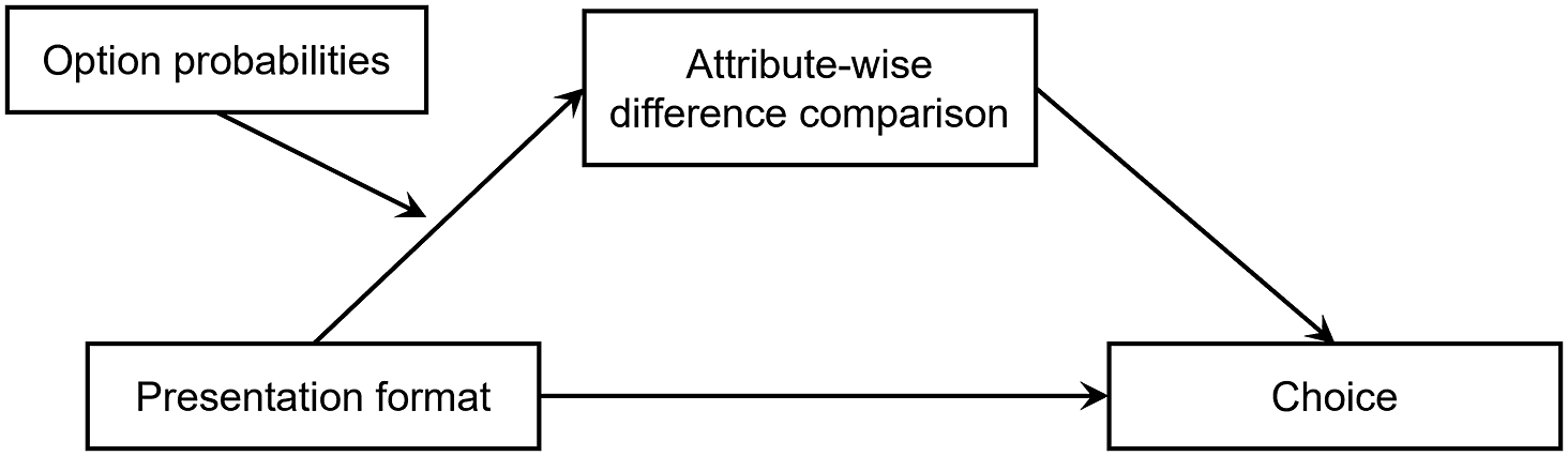
Figure 1 Mediated moderation model whereby the magnitude of option probabilities moderates the relationship between presentation format and attribute-wise difference comparison.
1.4. Overview of the present study
This article presents 3 studies to test the aforementioned hypotheses. In Study 1, we tested H ${_1}$
by examining the effect of the presentation format (PROB vs. TIME) on continuous risky decisions and the moderating effect of the magnitude of option probabilities. In Study 2, we further measured the attribute-wise difference comparisons and tested H
${_1}$
by examining the effect of the presentation format (PROB vs. TIME) on continuous risky decisions and the moderating effect of the magnitude of option probabilities. In Study 2, we further measured the attribute-wise difference comparisons and tested H ${_2}$
and H
${_2}$
and H ${_3}$
to examine the underlying mechanism. In Study 3, we examined the robustness of the effect of presentation format on continuous risky decisions in more natural decision situations.
${_3}$
to examine the underlying mechanism. In Study 3, we examined the robustness of the effect of presentation format on continuous risky decisions in more natural decision situations.
2. Study 1
In Study 1, we conducted an initial experiment to examine the effect of the presentation format on continuous risky decisions and test the moderating effect of the option probabilities on the relationship between presentation format and continuous risky decisions.
2.1. Method
2.1.1. Participants
The sample size was calculated based on our pilot study using the R function lmmpower in package ‘longpower’ (Donohue and Edland, Reference Donohue and Edland2016). The necessary sample size to achieve 99% power by using mixed-effects logistic regression is N = 99. A total of 124 participants were recruited from a university’s human subjects pool and took part in the study for 5 yuan (RMB; approximately US$0.7) in cash for participation, among which, 2 of them were excluded from the data analysis owing to the failure of passing the conscientiousness test, resulting in a final sample of 122 participants (M $_{age}$
= 30.8
$_{age}$
= 30.8 $\pm $
7.1 years; 53% female). The university ethics review board approved this study, and all the participants had provided prior written-informed consent.
$\pm $
7.1 years; 53% female). The university ethics review board approved this study, and all the participants had provided prior written-informed consent.
2.1.2. Task
The lottery task is one of the most commonly used tasks in the field of decision-making under risk (e.g., Kahneman and Tversky, Reference Kahneman and Tversky1979; Tversky and Fox, Reference Tversky and Fox1995). Accordingly, a hypothetical continuous lottery task was designed to investigate participants’ continuous risky decisions in the gain domain. In this task, participants were told to imagine that they would participate in a continuous lottery game. The lottery is drawn once a month with a constant likelihood of winning, and the amount of its prize is also constant. A participant would participate in the lottery every month until she/he won the prize. In the task, participants were presented with a pair of continuous lottery options and were asked to indicate their preferred one.
Participants completed 2 presentation format conditions. In the PROB condition, the winning likelihood of a continuous lottery was represented by the monthly winning probability, such as ‘the monthly winning probability is 0.3%’. In the TIME condition, the winning likelihood of a continuous lottery was represented by the average time of winning the lottery, such as ‘the average winning time is 27.8 years’.
2.1.3. Stimuli
The stimuli consisted of 2 conditions, where each had 35 pairs of options. One is the PROB condition, and the other is the TIME condition. The options in the 2 conditions were in one-to-one correspondence and can be converted into each other (i.e., if the monthly winning probability is p, then the average time of winning is 1 / p months). The average time was expressed in years in the TIME condition. All participants completed the same set of option pairs. The set of option pairs were generated under the following restriction: (1) the outcomes ranged from 1,000 to 50-million yuan; (2) the probabilities ranged from 0.001% to 50%; (3) there were no dominating options in each pair of options; and (4) the difference between the expectations of the 2 options is no more than 20 times (Table S1 in the Supplementary Material). Thus, in each pair of options, there are a safer option with a higher probability of winning but a smaller prize and a riskier option with a lower probability of winning but a bigger prize (see Figure 2 for an example). In addition, in each condition, there was a conscientiousness question, in which a dominating option in both attributes existed. If a participant did not choose the dominating option, then she/he was not devoted to the task and failed the conscientiousness test.
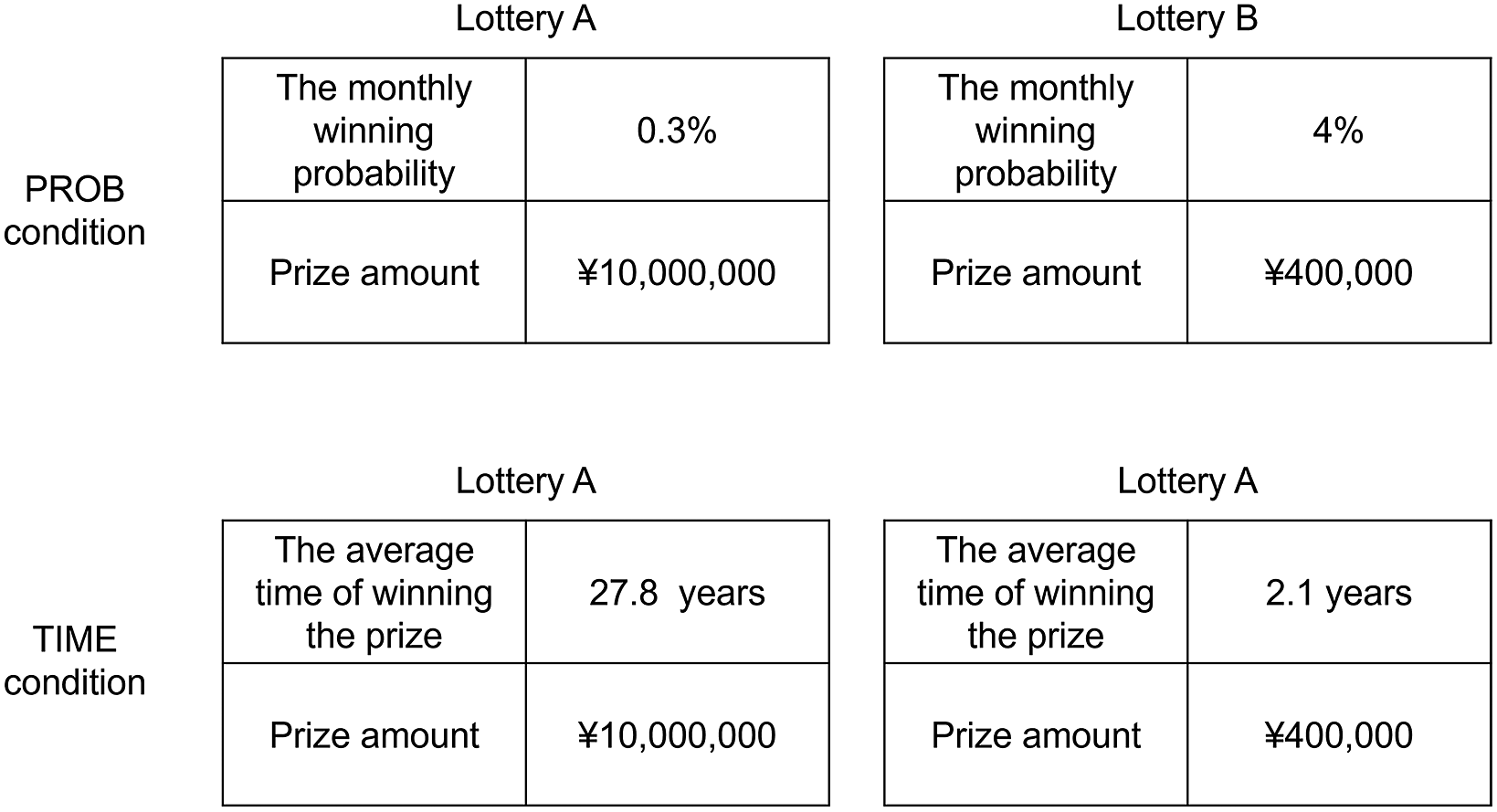
Figure 2 Example of the stimuli in Study 1.
2.1.4. Procedure
Participants first consented to take part in the experiment and were then told the rules of the task. Thereafter, they completed the choice task in the 2 conditions. The order of the conditions was counterbalanced across the participants. Half of the participants completed the PROB condition first, and the other half completed the TIME condition first. After finishing the choices in the first condition, participants had a break (1–2 min) and then started the second condition.
2.2. Results
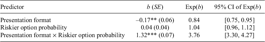
Participants’ choices were dummy coded (0 = choose the safe option, 1 = choose the risky option). On average, the percentage of choosing the risky option was 28.8% (95% CI = [27.8%, 29.8%]) overall, 29.4% (95% CI = [28.0%, 30.8%]) in the PROB condition, and 28.2% (95% CI = [26.8%, 29.5%]) in the TIME condition. A mixed-effects logistic regression was conducted to examine the effect of the presentation format and the option probabilities on continuous risky decisions. The model included the presentation format (dummy-coded, 0 = PROB condition, 1 = TIME condition), riskier option probabilities (continuous, standardized), and their interaction as fixed effects, including individual intercepts as a random effect. The results were shown in Table 1. As expected, the predicted 2-way interaction emerged significant. The results were shown in Table 1. Simple slope analyses revealed that within the gain domain, when the riskier option probability was at a small magnitude level (M – 1SD), participants were less likely to choose the risky option (b = –1.50, exp(b) = 0.22, 95% CI = [0.18, 0.27], z = –16.73, p $<$
0.001) when the options were presented in the TIME format than in the PROB format. On the contrary, when the riskier option probability was at a large magnitude level (M + 1SD), participants were more likely to choose the risky option (b = 1.15, exp(b) = 3.15, 95% CI = [2.66, 3.75], z = 13.02, p
$<$
0.001) when the options were presented in the TIME format than in the PROB format. On the contrary, when the riskier option probability was at a large magnitude level (M + 1SD), participants were more likely to choose the risky option (b = 1.15, exp(b) = 3.15, 95% CI = [2.66, 3.75], z = 13.02, p $<$
0.001) in the TIME format than in the PROB format. This finding supported H
$<$
0.001) in the TIME format than in the PROB format. This finding supported H ${_1}$
.
${_1}$
.
Table 1 Results from the mixed-effects logistic regression predicting continuous risky decisions in Study 1
Note: Values in the Exp(b) column represent the odds of selecting the risky options. Marginal $R^{2}$
= 0.11, Conditional
$R^{2}$
= 0.11, Conditional $R^{2}$
= 0.61,
$R^{2}$
= 0.61, $\chi ^{2}$
= 983.29***, predictive accuracy = 74.1%.
$\chi ^{2}$
= 983.29***, predictive accuracy = 74.1%.
** $p < 0.01$
.
$p < 0.01$
.
*** $p < 0.001$
.
$p < 0.001$
.
Given that the moderator is a continuous variable, the Johnson–Neyman technique (Hayes and Matthes, Reference Hayes and Matthes2009) was further used to probe the interaction through SPSS PROCESS macro 2.1.5 (Model 1) (Hayes, Reference Hayes2018). This technique can help to identify the boundaries of regions of significance, which defines the range of moderator values that the effect of the independent variable turns from statistically significant to not significant (Hayes, Reference Hayes2012). The results of the Johnson–Neyman technique on the moderated relationship between presentation format and continuous risky decisions were presented in Figure 3, which showed the effects (b) of presentation format on continuous risky decisions at different values of the riskier option probabilities. The results revealed that, within the gain domain, at a relatively low level of riskier option probabilities (riskier option’s probability of 2.21% and lower), participants were more likely to choose the risky option when the options were presented in the PROB format than in the TIME format. By contrast, at a relatively high level of riskier option probabilities (riskier option’s probability of 3.06% and higher), participants were more likely to choose the safe option when the options were presented in the PROB format than in the TIME format (Figure 3). The results supported H $_{1}$
.
$_{1}$
.
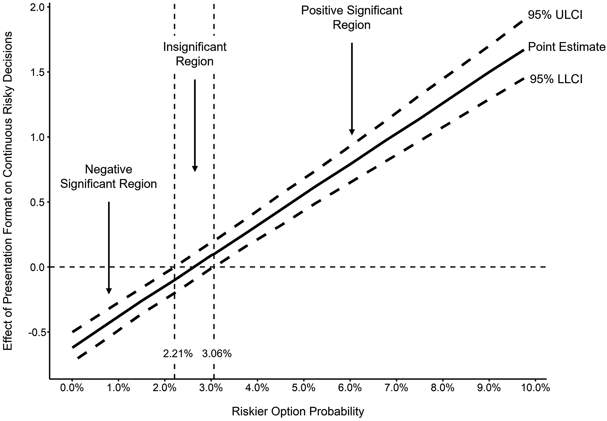
Figure 3 Johnson–Neyman significance regions for the moderated effect of the presentation format on continuous risky decisions in Study 1. The y-axis represents the regression coefficients of presentation format.
3. Study 2
In Study 1, we verified the moderating effect of the magnitude of option probabilities on the relationship between the presentation format and continuous risky decisions. In Study 2, we further examined the underlying mechanism and tested H ${_2}$
and H
${_2}$
and H ${_3}$
. As mentioned above, it is assumed that the attribute-wise difference comparisons mediate the effect of presentation format on continuous risky decisions. Therefore, in Study 2, we used a visual analog scale (VAS) paradigm (Jiang et al., Reference Jiang, Liu, Cai and Li2016; Kuang et al., Reference Kuang, Huang and Li2022) to measure the attribute-wise difference comparisons. In addition, the stimuli were more strictly controlled to ensure that the options can be classified into large and small probability conditions and that the expected values of the 2 options were equal.
${_3}$
. As mentioned above, it is assumed that the attribute-wise difference comparisons mediate the effect of presentation format on continuous risky decisions. Therefore, in Study 2, we used a visual analog scale (VAS) paradigm (Jiang et al., Reference Jiang, Liu, Cai and Li2016; Kuang et al., Reference Kuang, Huang and Li2022) to measure the attribute-wise difference comparisons. In addition, the stimuli were more strictly controlled to ensure that the options can be classified into large and small probability conditions and that the expected values of the 2 options were equal.
3.1. Method
3.1.1. Participants
We used the lmmpower function to calculate the required sample size based on the results of Study 1. The same with Study 1, we calculated the number of participants necessary to achieve 99% power by using mixed-effects logistic regression. The necessary sample size was N = 105. A total of 139 participants were recruited from a university’s human subjects pool and took part in the study for 7 yuan (RMB; approximately US$1.0) in cash for participation, among which 3 of them were excluded because of failure to pass the conscientiousness test. Therefore, a total of 136 participants (M $_{age}$
= 22.3
$_{age}$
= 22.3 $\pm $
3.2 years; 68% female) were included in the final analysis. The university ethics review board approved this research, and all the participants had provided prior written-informed consent.
$\pm $
3.2 years; 68% female) were included in the final analysis. The university ethics review board approved this research, and all the participants had provided prior written-informed consent.
3.1.2. Task
Similar to Study 1, the continuous lottery game task was used in Study 2. In the task, participants were presented with a pair of continuous lotteries and asked to indicate their preferred one. Then, the participants were also asked to indicate their subjective evaluation of the attribute-wise difference comparison using a 7-point VAS. The VAS was developed by Jiang et al. (Reference Jiang, Liu, Cai and Li2016) and has been used as an effective tool to compare the differences of the 2 options in each attribute to each other. The scale’s rating results can be used to identify which attribute shows a greater attribute-wise difference (Kuang et al., Reference Kuang, Huang and Li2022). In this VAS task, a scale was used to visually represent the comparison between the difference in the risk and outcome attributes ( $\Delta $
Risk
$\Delta $
Risk ${_{A,B}}$
/
${_{A,B}}$
/ $\Delta $
Outcome
$\Delta $
Outcome ${_{A,B}}$
). The difference between the 2 options in the risk attribute (
${_{A,B}}$
). The difference between the 2 options in the risk attribute ( $\Delta $
Risk
$\Delta $
Risk ${_{A,B}}$
) was placed on the left side of the scale, whereas that between the 2 options in the outcome attribute (
${_{A,B}}$
) was placed on the left side of the scale, whereas that between the 2 options in the outcome attribute ( $\Delta $
Outcome
$\Delta $
Outcome ${_{A,B}}$
) was placed on the right. If
${_{A,B}}$
) was placed on the right. If $\Delta $
Risk
$\Delta $
Risk ${_{A,B}}$
was evaluated as greater than
${_{A,B}}$
was evaluated as greater than $\Delta $
Outcome
$\Delta $
Outcome ${_{A,B}}$
, then the scale would tilt to the left (i.e., 1–3). If
${_{A,B}}$
, then the scale would tilt to the left (i.e., 1–3). If $\Delta $
Risk
$\Delta $
Risk ${_{A,B}}$
was evaluated as the same as
${_{A,B}}$
was evaluated as the same as $\Delta $
Outcome
$\Delta $
Outcome ${_{A,B}}$
, then the scale would not be tilted (i.e., 4). If
${_{A,B}}$
, then the scale would not be tilted (i.e., 4). If $\Delta $
Risk
$\Delta $
Risk ${_{A,B}}$
was evaluated as smaller than
${_{A,B}}$
was evaluated as smaller than $\Delta $
Outcome
$\Delta $
Outcome ${_{A,B}}$
, then the scale would tilt to the right (i.e., 5–7). The steeper the slope of the scale, the greater the attribute-wise difference between the attributes. Figure 4 shows the 7-point VAS for the PROB condition as an example.
${_{A,B}}$
, then the scale would tilt to the right (i.e., 5–7). The steeper the slope of the scale, the greater the attribute-wise difference between the attributes. Figure 4 shows the 7-point VAS for the PROB condition as an example.
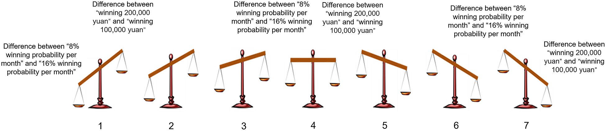
Figure 4 Schematic of the 7-point VAS used in the PROB condition in Study 2 as an example.
3.1.3. Design and stimuli
A 2 (presentation format: PROB vs. TIME) $\times $
2 (option probabilities: large vs. small) within-subject design was implemented. The stimuli included a block of trials in the PROB condition and a block of trials in the TIME condition. The options in the 2 conditions were in one-to-one correspondence and can be converted into each other. The time was expressed in months (e.g., 5 months) when it was less than 1 year; otherwise, the time was expressed in years plus months (e.g., 3 years and 5 months). This expression is commonly used in daily life, which may help participants evaluate the length of time. Each block contained 10 pairs of options in the large probability condition and 10 pairs of options in the small probability condition. According to the results in Study 1, the interval from 2.21% to 3.06% might be a key region where the effect of the presentation format on continuous risky decisions might shift the direction. Therefore, the option probabilities in the small probability condition were under 1%, and the option probabilities in the large probability condition were greater than 4%. The option pairs in the 2 probability conditions were also in one-to-one correspondence. The amount of prize was the same for the corresponding pairs of options, but the probability of the options in the large probability condition was 100 times higher than the probability of the corresponding options in the small probability condition (Table S2 in the Supplementary Material). In addition, similar to Study 1, a conscientiousness question also exists to check whether the participants were devoted to the task.
$\times $
2 (option probabilities: large vs. small) within-subject design was implemented. The stimuli included a block of trials in the PROB condition and a block of trials in the TIME condition. The options in the 2 conditions were in one-to-one correspondence and can be converted into each other. The time was expressed in months (e.g., 5 months) when it was less than 1 year; otherwise, the time was expressed in years plus months (e.g., 3 years and 5 months). This expression is commonly used in daily life, which may help participants evaluate the length of time. Each block contained 10 pairs of options in the large probability condition and 10 pairs of options in the small probability condition. According to the results in Study 1, the interval from 2.21% to 3.06% might be a key region where the effect of the presentation format on continuous risky decisions might shift the direction. Therefore, the option probabilities in the small probability condition were under 1%, and the option probabilities in the large probability condition were greater than 4%. The option pairs in the 2 probability conditions were also in one-to-one correspondence. The amount of prize was the same for the corresponding pairs of options, but the probability of the options in the large probability condition was 100 times higher than the probability of the corresponding options in the small probability condition (Table S2 in the Supplementary Material). In addition, similar to Study 1, a conscientiousness question also exists to check whether the participants were devoted to the task.
3.1.4. Procedure
Similar to Study 1, participants first consented to take part in the experiment and were then told the rules of the choice task and the VAS task. Participants were also asked to answer the question as required to check whether they understood the rules of the VAS task (see the Supplementary Material for details), which is similar to previous studies (Kuang et al., Reference Kuang, Huang and Li2022). If a participant did not answer the question correctly, she/he would re-read the instructions until she/he answered the question correctly. Thereafter, the participants completed the choice and the VAS tasks. For each item, they first chose their preferred lottery option (choice task), and then immediately rated the attribute-wise difference comparison (VAS task). Each participants completed the 2 tasks in the 2 presentation format conditions, respectively. The order of the conditions was counterbalanced across the participants. Half of the participants completed the PROB condition first, and the other half completed the TIME condition first. After finishing the choice and the VAS tasks in the first condition, participants had a break (1–2 min) and then started the second condition.
3.2. Results
3.2.1. Choice
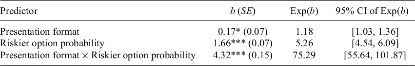
Similar to Study 1, participants’ choices were dummy coded (0 = choose the safe option, 1 = choose the risky option). On average, the percentage of participants choosing the risky option was 45.9% (95% CI = [44.5%, 47.2%]) overall, 44.1% (95% CI = [42.3%, 46.0%]) in the PROB condition and 47.6% (95% CI = [45.7%, 49.5%]) in the TIME condition. Participants’ choices were submitted to a mixed-effects logistic regression with the presentation format (0 = PROB condition, 1 = TIME condition), the magnitude of the option probabilities (0 = small, 1 = large), and their interaction as fixed effects, including individual intercepts as a random effect. The results were shown in Table 2. A significant interaction between the presentation format and option probabilities was found, which showed that within the gain domain, participants were less likely to choose the risky option (b = –1.99, exp(b) = 0.14, 95% CI = [0.11, 0.17], z = –18.90, p $<$
0.001) when the options were presented in the TIME format than in the PROB format at a small magnitude level of option probabilities. On the contrary, at the large magnitude level of option probability, participants were more likely to choose the risky option (b = 2.33, exp(b) = 10.26, 95% CI = [8.33, 12.64], z = 21.90, p
$<$
0.001) when the options were presented in the TIME format than in the PROB format at a small magnitude level of option probabilities. On the contrary, at the large magnitude level of option probability, participants were more likely to choose the risky option (b = 2.33, exp(b) = 10.26, 95% CI = [8.33, 12.64], z = 21.90, p $<$
0.001) when the options were presented in the TIME format than in the PROB format (Figure 5a). The results were consistent with Study 1, supporting H
$<$
0.001) when the options were presented in the TIME format than in the PROB format (Figure 5a). The results were consistent with Study 1, supporting H ${_1}$
.
${_1}$
.
Table 2 Results from the mixed-effects logistic regression predicting continuous risky decisions in Study 2
Note: Values in the Exp(b) column represent the odds of selecting the risky options. Marginal $R^{2}$
= 0.25, conditional
$R^{2}$
= 0.25, conditional $R^{2}$
= 0.55,
$R^{2}$
= 0.55, $\chi ^{2}$
= 1,433.10***, predictive accuracy = 68.3%.
$\chi ^{2}$
= 1,433.10***, predictive accuracy = 68.3%.
*p $<$
0.05.
$<$
0.05.
***p $<$
0.001.
$<$
0.001.
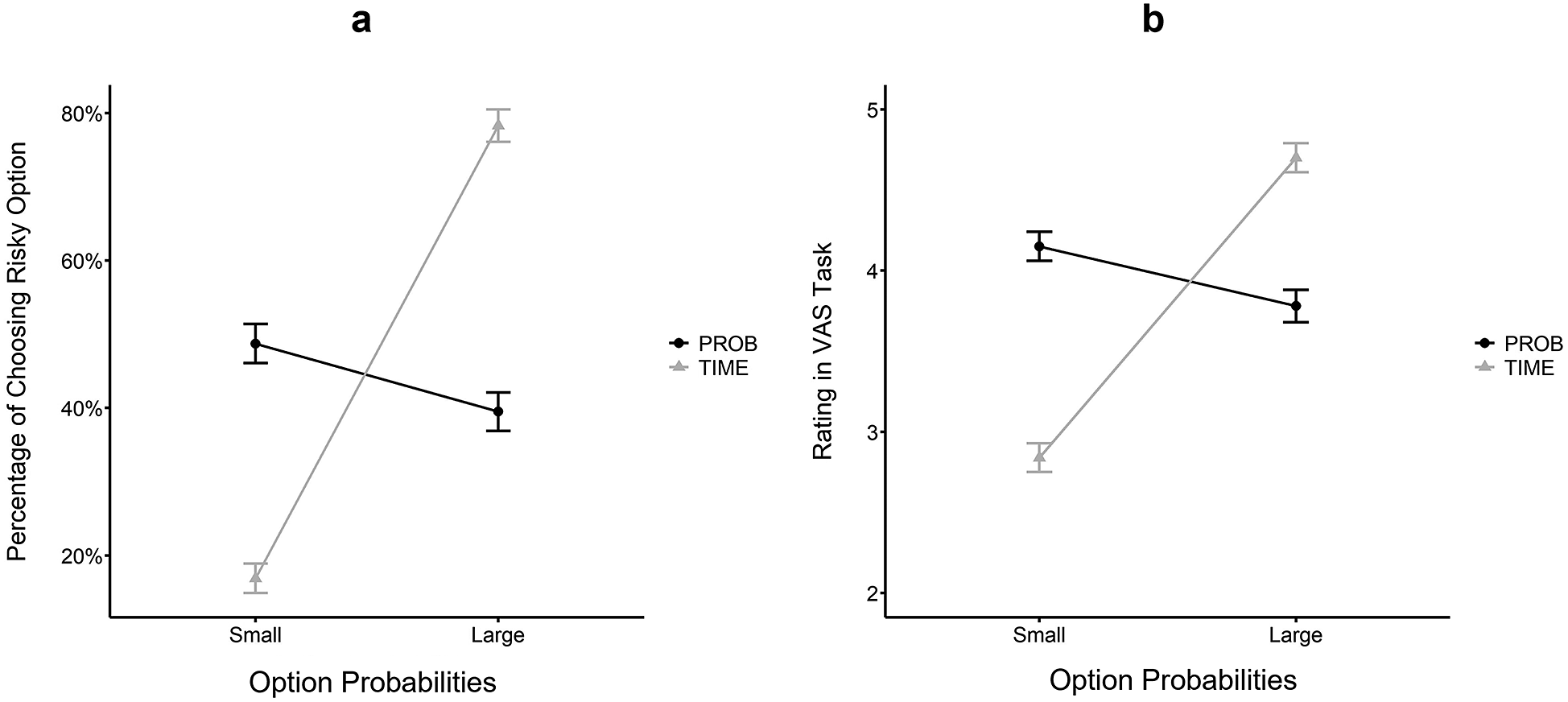
Figure 5 Results in Study 2. (a) The moderating effect of option probabilities on continuous risky decisions. (b) The moderating effect of option probabilities on attribute-wise difference comparisons. A lower score of VAS rating indicated that $\Delta $
Risk
${_{A,B}}$
is evaluated as much bigger than
$\Delta $
Risk
${_{A,B}}$
is evaluated as much bigger than $\Delta $
Outcome
$\Delta $
Outcome ${_{A,B}}$
, whereas a higher score of VAS rating indicated that
${_{A,B}}$
, whereas a higher score of VAS rating indicated that $\Delta $
Risk
$\Delta $
Risk ${_{A,B}}$
is evaluated as much smaller than
${_{A,B}}$
is evaluated as much smaller than $\Delta $
Outcome
$\Delta $
Outcome ${_{A,B}}$
. Error bars represent 95% CI.
${_{A,B}}$
. Error bars represent 95% CI.
3.2.2. Attribute-wise difference comparison
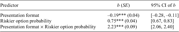
Participants’ evaluations of the attribute-wise difference comparisons were submitted to a mixed-effects linear regression with the presentation format (0 = PROB condition, 1 = TIME condition), the magnitude of the option probabilities (0 = small, 1 = large), and their interaction as fixed effects, including individual intercepts as a random effect. The results were shown in Table 3. The analysis revealed the predicted interaction, and the simple effects analysis revealed that within the gain domain, participants tended to evaluate the risk attribute difference as bigger (b = –1.31, 95% CI = [–1.43, –1.19], t = –21.5, p $<$
0.001) when the options were presented in the TIME format than in the PROB format at the small magnitude level of the option probabilities. On the contrary, at the large magnitude level of option probabilities, participants evaluate the risk attribute difference as smaller (b = 0.92, 95% CI = [0.80, 1.04], t = 15.2, p
$<$
0.001) when the options were presented in the TIME format than in the PROB format at the small magnitude level of the option probabilities. On the contrary, at the large magnitude level of option probabilities, participants evaluate the risk attribute difference as smaller (b = 0.92, 95% CI = [0.80, 1.04], t = 15.2, p $<$
0.001) when options were presented in the TIME format than in the PROB format (Figure 5b). The results supported H
$<$
0.001) when options were presented in the TIME format than in the PROB format (Figure 5b). The results supported H ${_2}$
.
${_2}$
.
Table 3 Results from the mixed-effects logistic regression predicting continuous risky decisions in Study 2
Note: Marginal $R^{2}$
= 0.14, conditional
$R^{2}$
= 0.14, conditional $R^{2}$
= 0.25,
$R^{2}$
= 0.25, $\chi ^{2}$
= 914.92***.
$\chi ^{2}$
= 914.92***.
***p $<$
0.001.
$<$
0.001.
3.2.3. Mediated moderation model
The PROCESS macro (Model 7) (Hayes, Reference Hayes2013) with 5,000-sample bootstrapped 95% confidence intervals was used to test whether the moderating effect of option probabilities on the relationship between presentation format and continuous risky decisions is mediated by the attribute-wise difference comparisons. The results showed that the index of mediated moderation was significant (effect = 1.70, 95% CI = [1.50, 1.90]). More specifically, within the gain domain, the presentation format had a significant negative indirect effect on continuous risky decisions via the attribute-wise difference comparisons (b = –1.00, 95% CI = [–1.13, –0.88]) when the option probabilities were small. By contrast, the indirect effect was significantly positive (b = 0.70, 95% CI = [0.59, 0.82]) when the option probabilities were large. See Figure 6 for details. The results supported H $_{3}$
.
$_{3}$
.
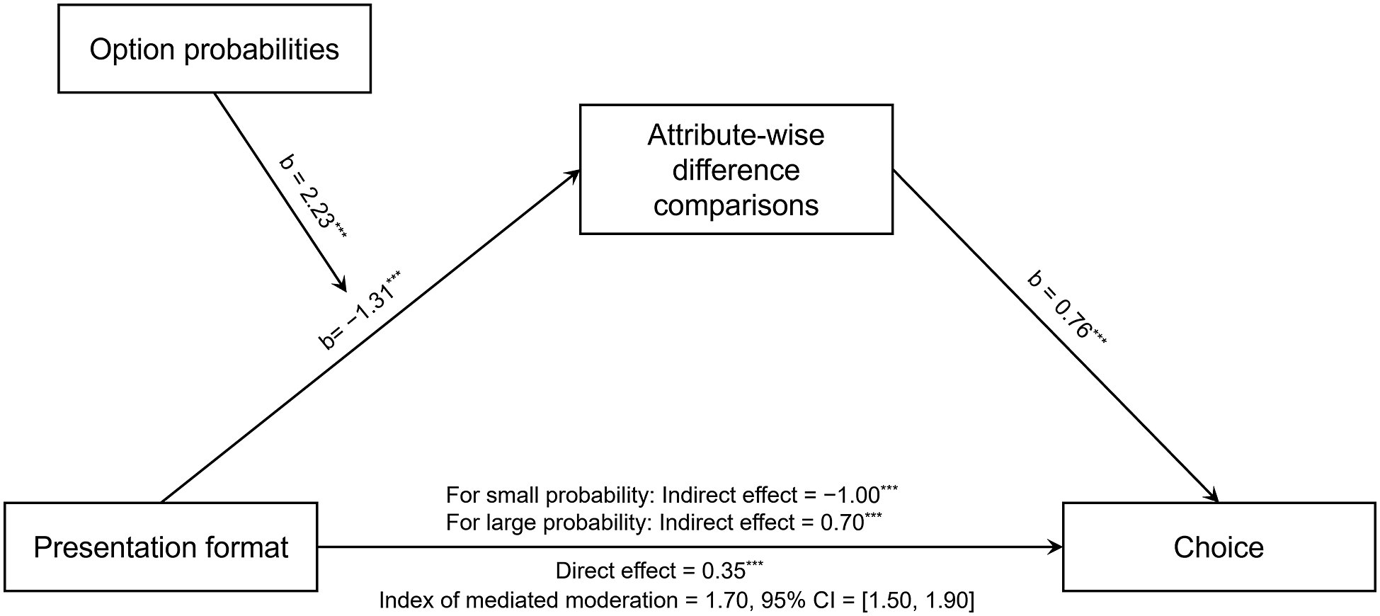
Figure 6 Moderated mediation analysis in Study 2. The effect of presentation format on continuous risky decisions was mediated by the attribute-wise difference comparisons. This mediation was moderated by option probabilities. $^{***}$
p
$^{***}$
p $<$
0.001.
$<$
0.001.
4. Study 3
The results in Studies 1 and 2 consistently revealed the effect of presentation format on continuous risky decisions. However, the decision scenarios in these 2 studies are relatively abstract and simple. Accordingly, in Study 3, we tested the effect of presentation format on continuous risky decisions in more natural scenarios to verify the robustness of this effect across different decision situations.
4.1. Method
4.1.1. Participants
G*Power (Version 3.1.9.2) (Faul et al., Reference Faul, Erdfelder, Lang and Buchner2007) is used to calculate the required number of participants to achieve 99% power and detect an effect size of Cohen’s f = 0.16 (the minimal effect size of Study 2) with a mixed ANOVA. The required sample size was N = 190. Therefore, a total of 221 participants (M $_{age}$
= 31.5
$_{age}$
= 31.5 $\pm $
8.1 years; 49% female) were recruited through online data collection platforms and took part in the study for 10 yuan (RMB; approximately US$ 1.4) in cash for participation. The university ethics review board approved this research, and all the participants had provided prior written-informed consent.
$\pm $
8.1 years; 49% female) were recruited through online data collection platforms and took part in the study for 10 yuan (RMB; approximately US$ 1.4) in cash for participation. The university ethics review board approved this research, and all the participants had provided prior written-informed consent.
4.1.2. Design and scenarios
A 2 $\times $
2 mixed design was implemented, with the presentation format (PROB vs. TIME) as a between-group factor and the scenarios (small probability scenario vs. large probability scenario) as a within-group factor. Two scenarios were designed based on real-life situations of continuous risk decisions. One was the car purchase scenario (small probability scenario), and the other was the cost-free house scenario (large probability scenario).
$\times $
2 mixed design was implemented, with the presentation format (PROB vs. TIME) as a between-group factor and the scenarios (small probability scenario vs. large probability scenario) as a within-group factor. Two scenarios were designed based on real-life situations of continuous risk decisions. One was the car purchase scenario (small probability scenario), and the other was the cost-free house scenario (large probability scenario).
The car purchase scenario was adopted based on real car licence plate policies in Tianjin, China. Participants were asked to imagine that they planned to buy a new car. However, the licence plate needs to be obtained through the licence plate lottery, which is drawn once a month. People who apply a licence plate will participate in the lottery every month until they win the licence plate. Participants were told that there were 2 different lotteries: Lottery A and Lottery B. Lottery A could win a licence plate of fuel vehicle. Ordinary fuel vehicles had a wide range of price points, but the winning likelihood was relatively low. The winning likelihood was 0.47% per month (in the TIME condition, participants were told that ‘the average time for the participants to win a licence plate is about 17 years and 9 months’). Then, Lottery B could win a licence plate of fuel-efficient car. The fuel-efficient cars were hybrid electric cars with a fuel-saving rate of more than 20%. Such fuel-efficient cars available for purchase were limited, and their prices were on the high side (most are more than 100,000 yuan). However, the fuel-efficient cars cost less fuel, and the winning likelihood was relatively high. The winning likelihood was 13.98% per month (in the TIME condition, participants were told that ‘the average time for the participants to win a licence plate is about 7 months’). The participants were asked to indicate which lottery they preferred using numbers 1–6 (1 = prefer Lottery A very much, 6 = prefer Lottery B very much).
The cost-free house scenario was adopted based on real employee welfare plans of some big companies (e.g., Alibaba and GAC Group) in China. Participants were asked to imagine that they worked for a large company and were awarded as ‘Excellent Star’ for outstanding performance. The ‘Excellent Star’ employee could participate in the cost-free house lottery. The lottery draws once a month, and the ‘Excellent Star’ employee can participate in the lottery every month until she/he win a house for free. Participants were told that there were 2 different lotteries: Lottery A and Lottery B. Lottery A could win a free house valued at 2–3-million yuan. The winning probability was 4% per month (in the TIME condition, participants were told that ‘the average time for the participants to win was about 1 year and 1 month’). Lottery B could win a free house valued at 1–1.5-million yuan. The winning probability was 40% per month (in the TIME condition, participants were told that ‘the average time for the participants to win was about 2.5 months’). The participants were asked to indicate which lottery they preferred using numbers 1–6 (1 = prefer Lottery A very much, 6 = prefer Lottery B very much).
4.1.3. Task and procedure
Participants needed to read the scenarios and answer the questions following each scenario. The order of the scenarios was counterbalanced across the participants.
4.2. Results
A 2 (presentation format: PROB vs. TIME) $\times $
2 (scenario: small probability scenario vs. large probability scenario) mixed design ANOVA was conducted, and the results showed no significant main effect. However, the interaction effect was found significant as expected, with F(1, 219) = 27.30, p < 0.001,
$\times $
2 (scenario: small probability scenario vs. large probability scenario) mixed design ANOVA was conducted, and the results showed no significant main effect. However, the interaction effect was found significant as expected, with F(1, 219) = 27.30, p < 0.001, $\eta ^{2}$
= 0.04. Simple effect analyses revealed that in the small probability scenario (the car purchase scenario), the preference scores in the PROB format condition (M = 3.69, 95% CI = [3.39, 3.99]) were significantly lower than those in the TIME format condition (M = 4.29, 95% CI = [4.02,4.56]), with t(219) = –2.92, p = 0.004, Cohen’s d = –0.39. By contrast, in the large probability scenario (the cost-free house scenario), the preference scores in the PROB format condition (M = 4.31, 95% CI = [4.02, 4.60]) were significantly higher than those in the TIME format condition (M = 3.60, 95% CI = [3.27, 3.92]), with t(219) = 3.19, p = 0.002, Cohen’s d = 0.43 (Figure 7). The results indicated that in the small probability scenario (the car purchase scenario), people were more likely to choose the safe option (the lottery to win the fuel-efficient car licence plate with a higher winning likelihood) when the likelihoods were presented in the TIME format than in the PROB format. By contrast, in the large probability scenario (the welfare housing scenario), participants were more likely to choose the risky option (the lottery to win a house valued at a higher price with a lower winning likelihood) when the likelihoods were presented in the TIME format than in the PROB format. These results were consistent with Studies 1 and 2, confirming the robustness of the effect in more natural decision situations.
$\eta ^{2}$
= 0.04. Simple effect analyses revealed that in the small probability scenario (the car purchase scenario), the preference scores in the PROB format condition (M = 3.69, 95% CI = [3.39, 3.99]) were significantly lower than those in the TIME format condition (M = 4.29, 95% CI = [4.02,4.56]), with t(219) = –2.92, p = 0.004, Cohen’s d = –0.39. By contrast, in the large probability scenario (the cost-free house scenario), the preference scores in the PROB format condition (M = 4.31, 95% CI = [4.02, 4.60]) were significantly higher than those in the TIME format condition (M = 3.60, 95% CI = [3.27, 3.92]), with t(219) = 3.19, p = 0.002, Cohen’s d = 0.43 (Figure 7). The results indicated that in the small probability scenario (the car purchase scenario), people were more likely to choose the safe option (the lottery to win the fuel-efficient car licence plate with a higher winning likelihood) when the likelihoods were presented in the TIME format than in the PROB format. By contrast, in the large probability scenario (the welfare housing scenario), participants were more likely to choose the risky option (the lottery to win a house valued at a higher price with a lower winning likelihood) when the likelihoods were presented in the TIME format than in the PROB format. These results were consistent with Studies 1 and 2, confirming the robustness of the effect in more natural decision situations.
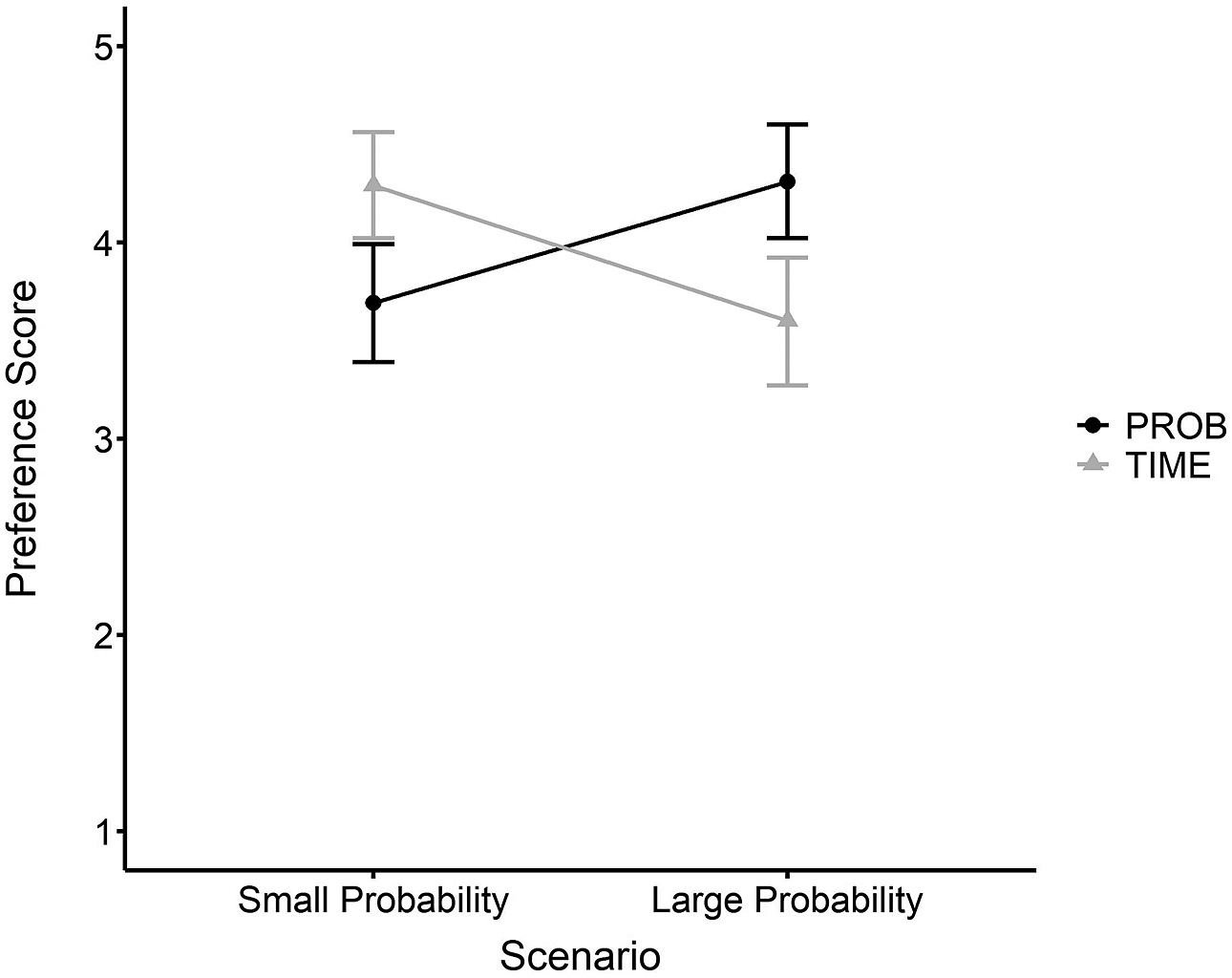
Figure 7 The effect of presentation format and scenario on preference scores in Study 3. A higher preference score indicated that participants were more likely to choose the safe option. Error bars represent 95% CI.
5. Discussion
In the present research, we examined the effect of presentation format on continuous risky decisions within the gain domain, and further explored the moderating effect of option probabilities and the mediating effect of attribute-wise difference comparisons. In Study 1, we found that within the gain domain, the magnitude of option probabilities moderated the effect of the presentation format on continuous risky decisions. Specifically, when the option probabilities are at a small level, individuals are more likely to choose the safe option in the TIME presentation format compared with the PROB presentation format. However, when the option probabilities are at a large level, individuals are more likely to choose the risky option in the TIME presentation format compared with the PROB presentation format. In Study 2, we further found that the moderating effect of the option probabilities on continuous risky decisions was mediated by the subjective attribute-wise difference judgment. In Study 3, we verified the effect of presentation format on continuous risky decisions in more natural and ecological decision scenarios.
5.1. Theoretical implications
In the field of risky decision-making, most of the research concentrated on the non-repeated one-shot risky choice but rarely considered the persistence of continuous risk events. The present study investigated continuous risky decisions within the gain domain, revealed the characteristic of the effect of presentation format on the decisions, and further examined the underlying mechanism. The present research helped us have a deep understanding of the mechanism of continuous risky decisions, and the results were conducive to further developing theories in relevant fields.
First, our findings revealed the pattern of the effect of the presentation format on continuous risky decisions within the gain domain. Several previous studies examined the difference between PROB and TIME presentation formats when describing continuous risky events. However, these studies used simple questionnaires to investigate people’s risk perception, lacking exact experimental control. For example, Bell and Tobin (Reference Bell and Tobin2007) investigated residents’ perception of flood risk through a questionnaire survey and found that the TIME format induced higher levels of concern and more of a need for protection than the PROB format. By using more exact experimental manipulations, the present study revealed that within the gain domain, the magnitude of option probabilities can moderate the effect of the presentation format on continuous risky decisions. For low-probability continuous risk events with positive outcome, the TIME format can decrease individuals’ risk-taking tendencies. By contrast, for the large probability of continuous risk events with desired outcome, the TIME format may increase people’s risk-taking behaviour. Our findings extended previous evidence and revealed the influence pattern of the presentation format on continuous risky decisions. These results suggest the boundary condition of this influence pattern.
Second, our findings revealed the underlying mechanism of the impact of the presentation format on continuous risky decisions within the gain domain. In this study, we found that the attribute-wise difference comparisons mediated the effect of the presentation format on continuous risky decisions, supporting the attributewise decision models (Li, Reference Li2004, 2016). Visschers et al. (Reference Visschers, Meertens, Passchier and de Vries2009) argued that people process continuous risk information heuristically instead of systematically to reach an evaluation. Given that the attribute-wise models are mostly heuristic theories, our findings are theoretically consistent with previous research. Continuous risky decisions are risky decisions with persistence. When a continuous risky decision was presented in the PROB format, it can be seen as a risky choice. However, when it was presented in the TIME format, it can be seen as an intertemporal choice. Researchers proposed that risky choice and intertemporal choice may share a common decision process at the cognitive computational level (Green et al., Reference Green, Myerson and Ostaszewski1999; Weber and Huettel, Reference Weber and Huettel2008) and can both be described by attribute-wise models (Leland, Reference Leland2002; Li, Reference Li2004, 2016; Rubinstein, Reference Rubinstein1988). Our findings suggest that when the probabilities and delays can be converted into each other, they may share the same cognitive mechanism. This case indicates the strong explanatory power and wide applicability of attribute-wise models.
Third, our findings suggest the varied sensitivities to risk and time information in continuous risky decisions within the gain domain. The range of probabilities in the PROB format is [0, 1], whereas the range of delays in the TIME format is far larger. This perception characteristic of time information results in that individuals are more sensitive to the risk attribute information in the TIME format compared with the PROB format. Given that the TIME presentation format makes it explicit how long people might wait for the desired outcome, the risk information is easier to be perceived and estimated in the TIME format compared with the PROB format (Li, Reference Li2016). Therefore, it is precisely because of the difference in the sensitivity of risk information among the 2 presentation formats that there is an interaction effect between presentation format and option probabilities. It is worth noting that for extremely small probability (e.g., 0.08%), when it is represented in the TIME format, the average time of risk occurrence may exceed the human lifespan (e.g., 104 years), and thus the outcome is treated as an impossible event. Although individuals may exhibit more conservative and risk-aversive behaviours within gain domain, the pattern of the effect of presentation format on continuous risky decisions revealed in the present research would not change in this situation. In addition, previous research used the weighting function to describe individuals’ perceptions of probabilities (Kahneman and Tversky, Reference Kahneman and Tversky1979; Tversky and Kahneman, Reference Tversky and Kahneman1992) and used the discounting function to describe individuals’ perceptions of delays (Frederick et al., Reference Frederick, Loewenstein and O’donoghue2002; Loewenstein and Prelec, Reference Loewenstein and Prelec1992; Samuelson, Reference Samuelson1937). From this point of view, our findings may also be explained by the different functions of probabilities and delays assumed by these as-if models. Future studies may further develop descriptive theories incorporating presentation format to quantitatively model individuals’ continuous risky decisions.
5.2. Practical implications
Our findings can provide significant insight for risk communication practitioners and help to establish effective intervention strategies for continuous risky decisions. Previous work examined the effect of the presentation format, such as frequency, pictographs, and numeracy formats, on an individual’s risk perception (Trevena et al., Reference Trevena, Zikmund-Fisher, Edwards, Gaissmaier, Galesic, Han, King, Lawson, Linder, Lipkus, Ozanne, Peters, Timmermans and Woloshin2013). These findings have been effectively applied in risk communication practices in clinical medicine (Trevena et al., Reference Trevena, Zikmund-Fisher, Edwards, Gaissmaier, Galesic, Han, King, Lawson, Linder, Lipkus, Ozanne, Peters, Timmermans and Woloshin2013), natural disasters (Strathie et al., Reference Strathie, Netto, Walker and Pender2017), and other fields. Given that the continuous risky decisions also involve many important areas related to policymaking and national welfare, the results in the present research can provide new insight into risk communication strategies for these areas.
In recent years, nudges have attracted extensive attention from psychological researchers, numerous governments, and international organizations (Hertwig and Grune-Yanoff, Reference Hertwig and Grune-Yanoff2017). Nudges are nonregulatory and nonmonetary interventions that steer people in a particular direction while preserving their freedom of choice (Thaler and Sunstein, Reference Thaler and Sunstein2008). A nudge is a new idea and new scheme provided by behavioural decision-making researchers to solve social problems (Li and Chapman, Reference Li and Chapman2013). Our findings may help to build a nudge study. Taking the licence plate lottery as an example, the government increased the lottery winning rate of fuel-efficient vehicles to 30 times that of ordinary fuel vehicles to encourage the citizens to buy more environmentally friendly energy-saving fuel vehicles. However, under the PROB presentation format, the citizens do not ‘buy’ it. Our findings suggest that if the lottery rate was presented in the TIME format, more people might choose energy-saving vehicles. It should be noted that it is still unclear which presentation format leads to a better risk perception. Although this kind of communication strategy could also be applied in areas such as disaster and disease prevention, it should be careful when designing a nudge considering that people must be able to make informed choices in these areas, given that the nudges should avoid appearing manipulative (Wilkinson, Reference Wilkinson2012).
5.3. Limitations
Our work also has several limitations. First, the continuous risky decision task in Studies 1 and 2 only involved monetary options in a gain frame. Many continuous risky decisions we face in real life involve potential losses, such as deciding whether to engage in high-risk work or whether to live in disaster-prone areas. Several studies reported an asymmetry between gain and loss frames in risky and intertemporal choices (Kahneman and Tversky, Reference Kahneman and Tversky1979; Scholten and Read, Reference Scholten and Read2014; Sun et al., Reference Sun, Li, Chen, Zhao, Rao, Liang and Li2015; Thaler, Reference Thaler1981). Accordingly, future studies should further explore the effect of presentation format on continuous risky decisions in the loss domain. Second, the present research did not examine the individual difference in continuous risky decisions. In the data analysis, we adopted the mixed-effects model and treated participant number as a random effect to verify the universality of the effect. However, different individuals may have different sensitivities to risky probability (Lauriola et al., Reference Lauriola, Panno, Levin and Lejuez2014) and time perception (Zhou et al., Reference Zhou, Li and Liu2021). For example, someone may have low sensitivity to risk and time, and thus the presentation format may have a slight effect on her/his decisions. By contrast, others may be more sensitive to the risk and time, and their decision is more likely to be affected by the presentation format. Future studies may further explore relevant psychological traits that can reflect the susceptibility to the presentation format, to provide a further reference for building nudge research. Third, the present research did not examine the possible influence of time units on temporal perception. In the experiments, we used years or years plus months to characterize the length of time in the TIME format, which is commonly used in daily life and may be helpful to evaluate the length of time. However, the changes in time units may affect individuals’ temporal perception and decision-making behaviour (Chandran and Menon, Reference Chandran and Menon2004; LeBoeuf, Reference LeBoeuf2006). Although the effect of presentation format on continuous risky choice has been shown to be robust across 3 experiments, future studies may further examine whether this effect is contingent on a change in time units used to express expected time to outcome. Fourth, the scenario differences were not controlled strictly in Study 3. The 2 scenarios in Study 3 were derived from real-world context to achieve high external validity. However, these 2 scenarios differed not only in probabilities, but also in some other aspects, such as the attractiveness of the desired outcomes. The potential confounding factors may weaken the internal validity of Study 3. Future research may re-examine the effect of presentation format on continuous risky decisions in well-designed scenarios to further exclude other possible confounding factors.
6. Conclusion
In sum, within the gain domain, people behaved differently in continuous risky decisions in 2 of the presentation formats, and the differences were moderated by the magnitude of option probabilities. Specifically, within the gain domain, compared with the probability of occurrence per unit time, using the average time of risk occurrence to present the continuous risky options led to more risk-aversion decisions when the probabilities were relatively low and led to more risk-seeking decisions when the probabilities were relatively large. In addition, the attribute-wise difference judgment mediated the effect of presentation format on continuous risky decisions.
Data availability statement
Data from these 3 studies and the Supplementary Material are publicly available via the Open Science Framework (https://osf.io/9q3xv/).
Author contribution
Z.-H.W. and H.-Z.L. conceived and designed this study, analysed data, and wrote the paper. Z.-H.W., H.-Z.L., and X.-Z.W. designed experimental stimuli and procedures. L.-Q.J. implemented experimental protocols and collected data. All authors contributed to the article and approved the submitted version.
Funding statement
This research was supported by grants from the National Natural Science Foundation of China (72001158) and the Fundamental Research Funds for the Central Universities (63222045). The funders were not involved in the study design, data collection and analysis, decision to publish, or preparation of the manuscript.
Competing interest
The authors declare that the research was conducted in the absence of any commercial or financial relationships that could be construed as a potential competing interest.
Ethical standard
The studies involving human participants were reviewed and approved by the Institutional Review Board of Tianjin Normal University. The participants provided their written informed consent to participate in this study.


 Open access