


Introduction
Stratigraphic correlation and prediction of subsurface reservoirs in low net-to-gross fluvial deposits is challenging, particularly when limited data are available to produce stratigraphic models. Such sedimentary systems are often characterised by extensive floodplains with localised, major and minor channels. Numerous studies have focused on characterising and predicting such reservoir architecture via the characterisation and correlation of sandstones (e.g. Bridge et al., Reference Bridge, Jalfin and Georgieff2000; Törnqvist & Bridge, Reference Törnqvist and Bridge2002; Sahoo et al., Reference Sahoo, Gani, Gani, Hampson, Howell, Storms, Martinius and Buckley2020). However, the formation of channel belts is typified by internally-driven, ”autogenic” processes, such as channel avulsion, crevasse splaying, and channel migration (e.g. Beerbower, Reference Beerbower1964; Smith et al., Reference Smith, Cross, Dufficy and Clough1989; Stouthamer & Berendsen, Reference Stouthamer and Berendsen2007). These processes lead to lithological heterogeneity and poor three-dimensional sandstone connectivity. The correlation potential of sandstones is therefore relatively low using only wireline data.
True overbank deposits tend to include regionally consistent characters. Continuous floodplain surfaces related to palaeosols or coals seams can be used to subdivide and correlate stratigraphy. These deposits better record external, "allogenic” processes such as tectonics or base-level and climate changes related to orbital cycles (Davydov et al., Reference Davydov, Crowley, Schmitz and Poletaev2010; Jirásek et al., Reference Jirásek, Opluštil, Sivek, Schmitz and Abels2018; Noorbergen et al., Reference Noorbergen, Abels, Hilgen, Robson, de Jong, Dekkers, Krijgsman, Smit, Collinson and Kuiper2018; Opluštil et al., Reference Opluštil, Lojka, Rosenau, Strnad and Kędzior2019). Orbital forcing results in consistent vertical spacing of features and provides a tool for cyclostratigraphic correlation (e.g. De Jong et al., Reference de Jong, Nio, Smith and Böhm2007; Reference de Jong, Donselaar, Boerboom, Van Toorenenburg, Weltje and Van Borren2020; Nio et al., Reference Nio, Böhm, Brouwer, Jong and Smith2014). However, although used for correlation, the underlying climatic forcing mechanism remains mostly unused in reservoir modelling. The repetitive patterns of orbital forcing may hold valuable predictive capabilities where trends are laterally consistent. Recognising orbitally-forced patterns and integrating underlying conceptual models in subsurface workflows could improve well-to-well correlations. It may also allow identification of channel sandstone-prone stratigraphic intervals at a resolution not available by other means.
A suitable target to elaborate the cyclostratigraphic methodology is the Euramerican Upper Carboniferous deltaic and fluvial systems. These are well known for their repetitive nature and lateral continuity of coal seams. The cyclic arrangement of these sediments was recognised in the early 19th century (Weller, Reference Weller1930; Wanless & Weller, Reference Wanless and Weller1932) and referred to as "cyclothems". Cyclothems comprise an array of clastic, organic, and chemical/biochemical lithologies and are often interpreted the products of alternations between non-marine and marine depositional conditions. For a summary, see Fielding (Reference Fielding2021). The concept of cyclothems has been applied to a broad range of sedimentary successions, including successions without marine strata. The most widely accepted forcing mechanism for cyclothems is base-level change via glacio-eustatic control (e.g. Ramsbottom, Reference Ramsbottom1973; Hampson et al., Reference Hampson, Stollhofen and Flint1999; Heckel, Reference Heckel2008; Gibling et al., Reference Gibling, Rygel, Fielding, Frank, Isbell, Fielding, Frank and Isbell2008; Fielding et al., Reference Fielding, Nelson and Elrick2020; Fielding, Reference Fielding2021). Glacio-eustasy is driven by (palaeo-)polar ice volume changes controlled by orbital forcing, and radioisotopic dating of several sequences of cyclothems confirms such a link to orbital forcing (e.g. Davydov et al., Reference Davydov, Crowley, Schmitz and Poletaev2010; van der Belt et al., Reference van den Belt, van Hoof and Pagnier2015). Besides base-level changes, upstream sediment fluxes, and variations in mid-stream water and vegetation levels have also been proposed as mechanisms for cyclothem formation (Jirásek et al., Reference Jirásek, Opluštil, Sivek, Schmitz and Abels2018; Opluštil et al., Reference Opluštil, Lojka, Rosenau, Strnad and Kędzior2019, Reference Opluštil, Laurin, Hýlová, Jirásek, Schmitz and Sivek2022).
Smith and Joeckel (Reference Smith and Joeckel2020) demonstrated the potential for improved reservoir characterisation with a stratigraphic framework based on cyclothem correlations. In this example, limestones alternate with mudstones following coastline movement and display little lateral variation in cycle character. In the more fluvial domain, cycle character is more variable. The autogenic dynamics of a fluvial system cause lateral variation on the floodplains and the characteristics of any one cyclothem can be laterally divergent. The ability to recognise and decouple autogenic and allogenic imprints in cyclothems is essential in these systems.
The present study aims to evaluate the potential of climate stratigraphy for improved reservoir quality assessment in low net-to-gross deltaic to fluvial systems using cyclothems. To do so, the dominantly fluvial Westoe and Cleaver formations (Maurits Formation in the Dutch sector) in the Silverpit Basin (Southern North Sea) are chosen (Fig. 1). Cyclothems are well-documented here as sequences of claystone, mudstone, siltstone, sandstone, and coal arranged in vertically stacked packages with coarsening upwards trends (O’Mara & Turner, Reference O’Mara and Turner1999; Fig. 4b). The thickness of these repetitions does not vary markedly across the floodplain, ranging up to 15 m (Quirk, Reference Quirk1993; O’Mara & Turner, Reference O’Mara and Turner1999). They are interpreted as shallowing-upward successions starting with lake deposits overlain by crevasse splay and minor delta deposits, and eventually mire accumulations. A depositional mechanism related to base-level fluctuation is proposed where the lake deposits were gradually filled in response to an upwards decrease in accommodation space due to base-level fall. Subsequently, the infill was capped by the formation of mires which sustained until drowning by base-level rise (O’Mara & Turner, Reference O’Mara and Turner1999).
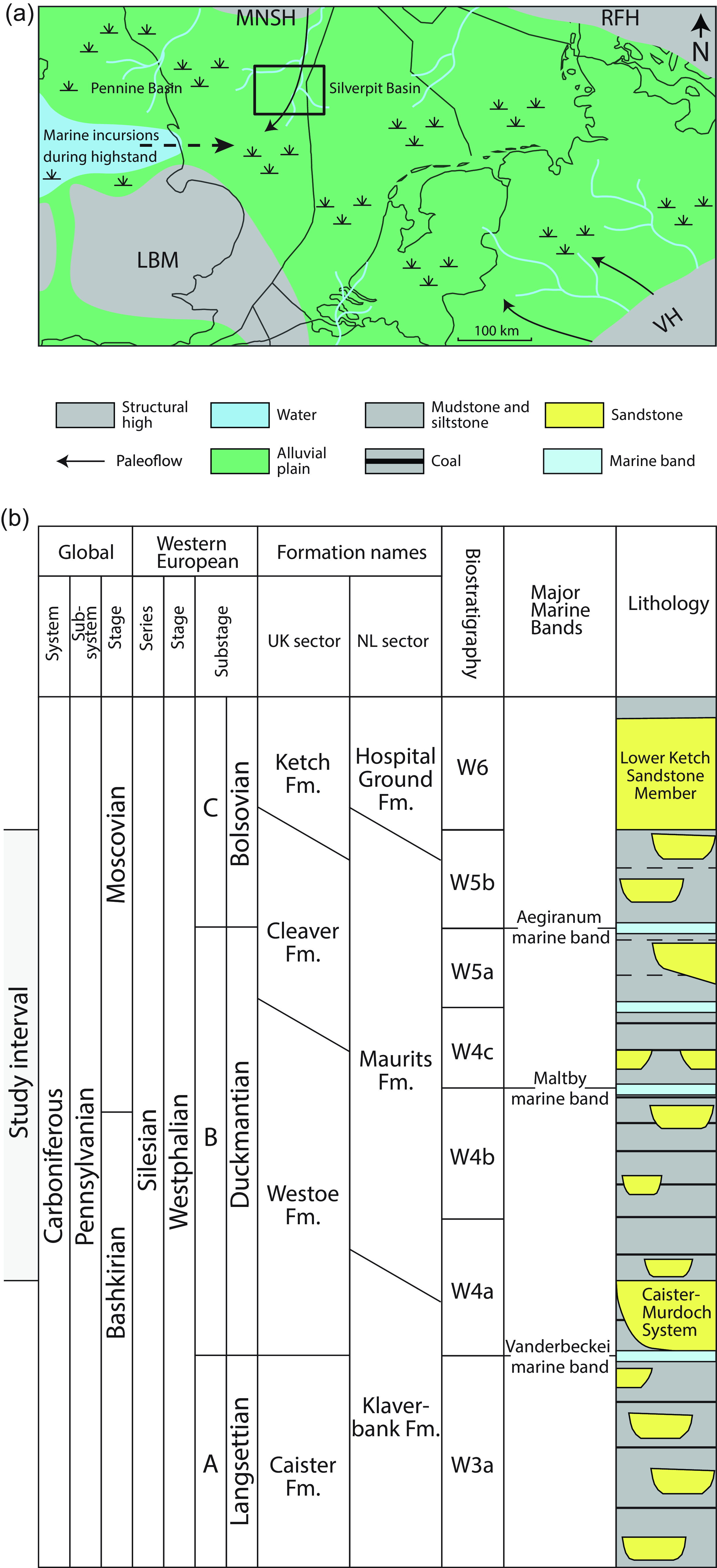
Figure 1. (a) Duckmantian palaeogeography of the UK, NL, and German sectors in the southern North Sea (modified after Doornenbal & Stevenson, Reference Doornenbal and Stevenson2010). Abbreviations: VH: Variscan Highlands, LBM: London-Brabant Massif, RFH: Ringkøbing-Fyn High, MNSH: Mid North Sea High. (b) Stratigraphic overview of the Westphalian for the study area. UK and Dutch offshore lithostratigraphy after Besly (Reference Besly, Collinson, Evans, Holliday and Jones2005) and Van Adrichem Boogaert & Kouwe (1995); miospore biozones after McLean et al. (Reference McLean, Owens and Neves2005); important marine bands after Ramsbottom et al. (Reference Ramsbottom1978) and generalised lithologies after Cameron et al. (Reference Cameron, Munns, Stoker, Collinson, Evans, Holliday and Jones2005). No vertical scale is implied.
Current correlation methods, such as bio-, chemo-, and (sandstone) litho-stratigraphy, provide stratigraphical resolution in the order of 50–100 m (Pearce et al., Reference Pearce, McLean, Martin, Ratcliffe, Wray, Ratcliffe and Zaitlin2010). Cyclothems with a thickness of <15 m, could provide much higher resolution for correlations. In this study: (1) cyclothems are identified per well, and variations in character are documented; (2) Manual and semi-automated methods are used to construct stratigraphic correlations based on the cyclothems; (3) The resulting horizontal and vertical sedimentary facies patterns are analysed; (4) These are combined with an analysis of sandstone occurrence and sandbody thickness and style; (5) Climate models are fitted to averaged stratigraphic trends, to identify stratigraphic intervals of higher reservoir potential.
Geological setting
The Silverpit Basin is one of several coal-bearing Carboniferous basins located north of the foreland of the Variscan Orogeny (Leeder, Reference Leeder1988). It is primarily located in UK offshore Quadrants 44 and 49, partly in the Netherlands Blocks D, E and J, and lies along the proximal northern margin of the more extensive Pennine Basin. Carboniferous strata ranging from Tournaisian to Westphalian (and possibly younger) were deposited as the basin formed a major sediment fairway from the northeast towards the south-southwest (Besly, Reference Besly, Besly and Kelling1988; Collinson et al., Reference Collinson, Jones, Blackbourn, Besly, Archard and McMahon1993; Cole et al., Reference Cole, Whittaker, Kirk and Crittenden2005). The primary sediment source was across the Mid North Sea High in the north, with occasional input from the Variscan Orogen to the southeast (Morton et al., Reference Morton, Claoué-Long and Hallsworth2001; Besly, Reference Besly, Collinson, Evans, Holliday and Jones2005). The depocentre is likely positioned in the southern part of Quadrant 44 (O’Mara, Reference O’Mara1995)
The Westoe and Cleaver formations are Duckmantian (Westphalian B) to early Bolsovian (Westphalian C). Most sediments in these formations were deposited on a low-relief alluvial plain setting with a distant coastline under a palaeoequatorial, perhumid palaeoclimate (O’Mara & Turner, Reference O’Mara and Turner1999). The succession is predominantly terrestrial and consists of clastic deposits ranging from sandstones to mudstones and coals. Sediment supply was by fluvial channels and overbank deposits fed by crevasse splay or minor delta systems that entered numerous inter-channel freshwater lakes (Haszeldine, Reference Haszeldine1983; Fielding, Reference Fielding1984a, Reference Fielding1986; Guion and Fielding, Reference Guion, Fielding, Besley and Kelling1988). The Westoe Formation is a shale-dominated succession with high organic content, abundant coal seams, limited sandstone occurrence, and very little marine influence. In the Cleaver Formation, coal occurrence slightly decreases, and sandstones and marine intervals are more common. Marine intervals are represented by thin marine mudstones (“marine bands”) interpreted as representing glacio-eustatic flooding events in sequence stratigraphic models (Calver, Reference Calver1968; O’Mara & Turner, Reference O’Mara and Turner1997).
The study interval is bounded between two regionally extensive major packages of stacked fluvial sandstones (Cameron et al., Reference Cameron, Munns, Stoker, Collinson, Evans, Holliday and Jones2005). The lowest part of the Westoe Formation at the base of the study interval is characterised by the stacked sandstones of the Caister-Murdoch system that overlies the Vanderbeckei Marine Band (MB). The top of the study interval is defined at the lower Ketch member of the Ketch Formation. The Aegiranum MB is located below the lower Ketch member. The major marine bands are interpreted as high-stand deposits. These are followed by concentrations of sandstones, which reflect periods of non-deposition and erosion succeeded by stacking fluvial system infills during low-stands (Huis in ‘t Veld et al., Reference Huis in’t Veld, Schrijver and Salzwedel2020). The base of the Cleaver Formation is identified by the Maltby MB Onshore sections in the Pennine Basin contain several thin marine bands indicating small marine incursions throughout the equivalents of the Cleaver Formation (Calver, Reference Calver1968). In the lower part of the Duckmantian the flooding surfaces are lacustrine rather than marine, as is evident from the fossil record (Trueman and Weir, Reference Trueman and Weir1946; Calver, Reference Calver1956; Eagar, Reference Eagar1954; O’Mara & Turner Reference O’Mara and Turner1997). Several timescales estimates, varying between 1.2 and 2.5 Myr, can be used for the duration between the formation of the Vanderbeckei MB and the Aegiranum MB (Davydov et al., Reference Davydov, Wardlaw and Gradstein2004; Menning et al., Reference Menning, Alekseev, Chuvashov, Davydov, Devuyst, Forke, Grunt, Hance, Heckel, Izokh, Jin, Jones, Kotlyar, Kozur, Nemyrovska, Schneider, Wang, Weddige, Weyer and Work2006; Van der Belt et al., Reference van den Belt, van Hoof and Pagnier2015; Opluštil et al., Reference Opluštil, Schmitz, Kachlík and Štamberg2016).
McLean, (Reference McLean1995), Besly (Reference Besly, Collinson, Evans, Holliday and Jones2005), and Waters et al. (Reference Waters, Collinson, McLean, Besly, Waters, Somerville, Jones, Cleal, Collinson, Waters, Besly, Dean, Stephenson, Davies, Freshney, Jackson, Mitchell, Powell, Barclay, Browne, Leveridge, Long and McLean2011) consider there to be a disconformity at the base Ketch Formation. The stratigraphy thins to the northeast and thickens to the southwest due to a rapidly subsiding basin depocentre in the southwest (Huis in ‘t Veld et al., Reference Huis in’t Veld, Schrijver and Salzwedel2020). This thinning trend, combined with increasing rates of incision of the Ketch Formation northwards, leads to a disconformity at the base of the Ketch, but this is supposed to be minimal in the study area. The constant thickness of the Westphalian interval and the absence of large incisions on seismic interpretations suggest that regional subsidence was relatively high and exceeded the stratigraphic base-level fall (Leeder, Reference Leeder1988; Turner et al., Reference Turner, Younger and Fordham1993). Additionally, the high correlatability of marine excursions over Europe (Dusar et al., Reference Dusar, Paproth, Streel and Bless2000) suggests that tectonic activity had a low impact on stratigraphic variability.
Methods
Data and transect
Two transects have been made perpendicular to the southwest thickening trend. In Transect One, fourteen wells cover a maximal lateral distance of 57 km from west to east. Transect Two, 12 km to the northeast, consists of five anonymised wells and spans approximately 15 km. Standard wireline suites of gamma-ray, density, sonic, and neutron-porosity logs were used for analysis. All wireline logs were corrected for environmental borehole conditions. The wells were adjusted for borehole and structural deviation and displayed at true stratigraphic thickness (TST). The base of the Variscan unconformity was used as a zero horizon for the stratigraphic thickness. Structural dip above the unconformity is assumed to be minimal, and the depth above the Variscan unconformity was added to the TST. Well 44/23-14 was capped at the highest matching biostratigraphic marker since seismic interpretations indicate a fault gap.
The study workflow is shown in Fig. 2. Three different approaches for the correlation of wells were applied: manual, semi-automatic, and stratigraphic thickness. Specific methods are explained below.

Figure 2. The workflow conducted in this study. Three different approaches to stratigraphic correlation are made: manual, semi-automatic, and stratigraphic thickness. The specific approaches are further explained in the text.
Existing stratigraphic markers
The transects are referenced to a well-established miospore biozonation for the area (McLean et al., Reference McLean, Owens and Neves2005). Archive biostratigraphic control was available for six of the selected wells, and, for consistency, all biostratigraphic data used in this study were provided by one analyst (MB Stratigraphy Limited). Four biozones are defined within the study interval (W4a up to W5a; Fig. 1b). The biozones are defined, where possible, on the highest stratigraphical occurrences of zonal taxa (McLean et al., Reference McLean, Owens and Neves2005). All samples are from ditch-cuttings material. Supplementary data S1 shows data for the wells with biostratigraphy, any uncertainty and comparison to the cyclostratigraphic framework.
Miospore species range limits are likely to be linked to palaeoclimatological changes such as marine incursions, and a close relationship between the biozonation and marine bands has been established (McLean et al., Reference McLean, Owens and Neves2005). The Maltby MB and Aegiranum MB are related to the tops of the W4b and W5a biozones, respectively (Fig. 1b).
Integrated deviation curve
Because the lithological expression of a cyclothem can vary from place to place, identifying individual cyclothems was aided by applying a deviation filter (DC) to the gamma-ray logs (Nio et al., Reference Nio, Brouwer, Smith, de Jong and Böhm2005). This method tracks spectral change and identifies "breakpoints" (i.e. points of change; Fig. 3). A similar approach has been successfully applied in the Southern North Sea for large-scale correlation of wells. (De Jong et al., Reference de Jong, Smith, Nio and Hardy2006; Reference de Jong, Donselaar, Boerboom, Van Toorenenburg, Weltje and Van Borren2020). For the calculation of the DC, an open-source Python script was used (Daely, Reference Daely2019).
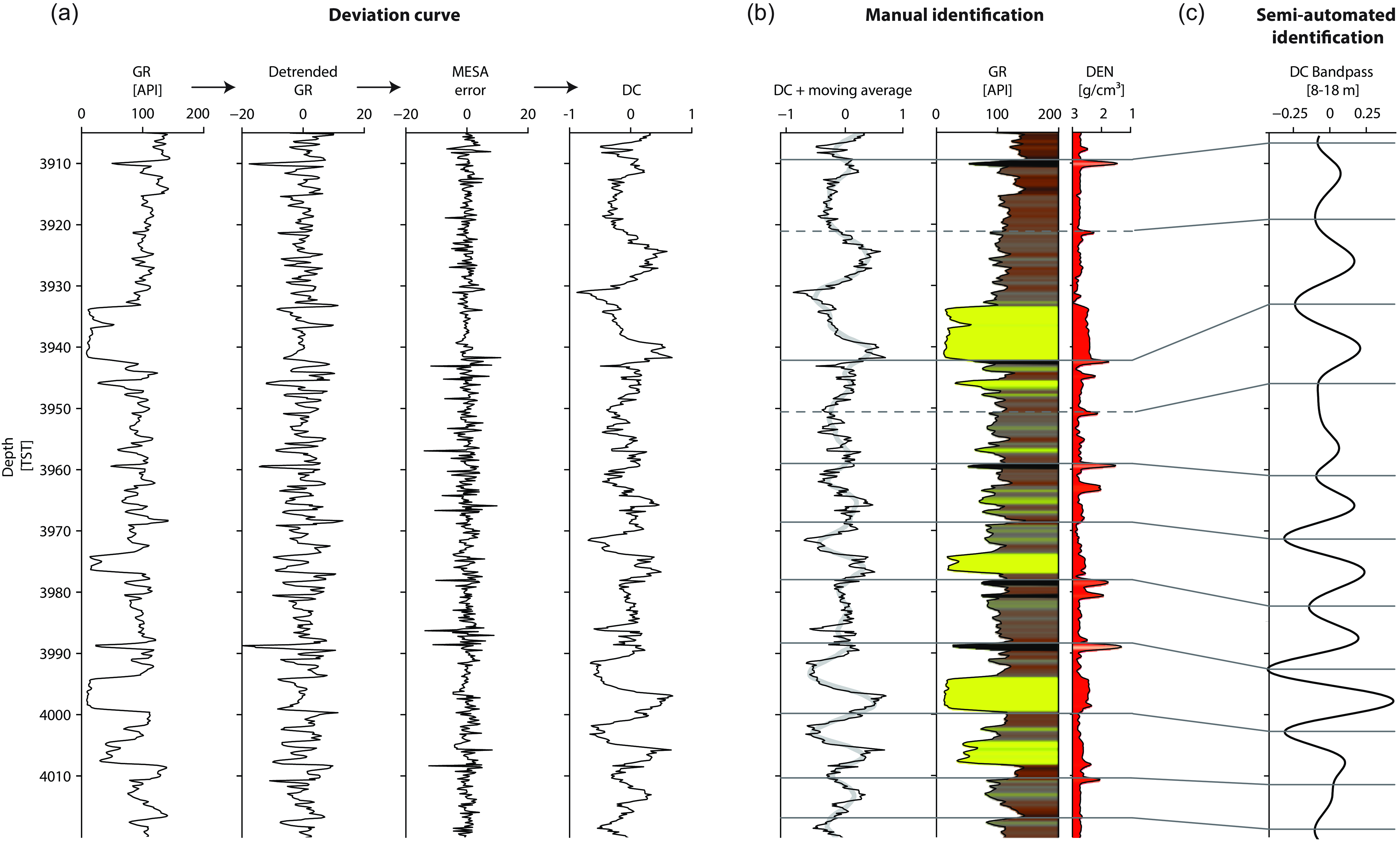
Figure 3. An example of the deviation curve methodology on the gamma-ray from well 44/22-8st. (a) The construction of the deviation curve. From left to right: The input gamma-ray record. The stacked L1 trend filters amplify smaller-scale spectral change and remove large-scale trends of the gamma-ray. The error of the signal prediction by the Maximum Entropy Analysis (MESA). The integration of the Burg method’s error shows the signal’s spectral trend attribute and periods of change on the breakpoints of the curve and is called the deviation curve (DC). (b) Manual identification of the cyclothems based on the gamma-ray and density record, combined with the visual aid of the deviation curve (moving average of the deviation curve is a Savitzky–Golay filter, 6 m, second polynomial). The colour fill of the gamma-ray is based on a continuous fill between 0 and 200 API values. Coals are coloured black and have a low API, like sandstone. Their identification is based on density values (<2.00 g/cm3). (c) Semi-automated identification of cyclothems based on a gaussian bandpass filter (6–18 m) of the deviation curve. The peaks of the bandpass filter are used as cyclothem boundaries.
An L1 trend filter method (Kim et al., Reference Kim, Koh, Boyd and Gorinevsky2009) was used to remove large-scale trends and to amplify small-scale trends before applying the DC analysis. This method is a high-pass filter, filtering out the low-frequency components. The strength of the filter is controlled by a regularisation parameter that balances the smoothness of the fit with the minimisation of smaller-scale variability between the actual signal and the smoothed series. A regularisation parameter of zero represents the original input signal, while the maximal regularisation parameter results in a linear signal. Twenty different filters were calculated with an exponentially increasing regularisation parameter between the maximal and minimal regularisation parameters. After calculating the L1-filters, the first twelve filtered high-frequency filters were combined, averaged, and subtracted from the original curve (Fig. 3b).
An autoregressive analysis in the form of a Maximum Entropy Analysis (MESA) was applied next (Burg, Reference Burg1967). This fits an autoregressive model to the signal by using least squares method to minimise the forward and backward prediction errors based on a defined window length. In this study the window length was 7 m. The error of the predicted model compared to the detrended gamma-ray indicates the unpredictability of a signal. This error provides valuable information about the stratigraphic change of the record. Further integration of the curve is termed the deviation curve (DC), indicating the spectral trend attribute of the signal and identifying points of change. The DC was smoothed by a moving average (Savitzky–Golay filter, 6 m, 2nd polynomial; Savitzky & Golay, Reference Savitzky and Golay1964).
Manual cycle identification
Gamma-ray logs are used as a substitute for grain size logs. Although grain size does not determine the natural gamma radiation, there is a dependency of mineral composition in grain size (i.e. Blatt et al., Reference Blatt, Middleton and Murray1980; Martinius et al., Reference Martinius, Geel and Arribas2002) which enables the recognition of coarsening- and fining-upwards trends. Coals can have similar low gamma-ray readings as sandstones, so the density curve was used for their identification. Coals generally have a significantly lower density and sonic travel time than other lithologies in the sections. A coal cut-off of >2.00 g/cm3 was used for most wells. Density readings were unavailable in wells 44/21-3 and 44/21-4. Here the neutron porosity (>0.45 m3/m3) and sonic (>80 μs/ft) readings were used, respectively.
A cyclothem boundary is defined at the base of a flooding surface. When coal is present, the boundary is placed at the top of the coal. However, cyclothems without coal development also occur. An approximated maximum geographical extent of 15–20 km was attributed to the coal seams which, due to paleotopographic variations, are not expected to have developed consistently over the whole basin (Haszeldine, Reference Haszeldine1983; Fielding, Reference Fielding1984a). Therefore, a boundary was placed at the transition from coarse-grained to fine-grained material in cyclothems without coal development.
The DC was used for visual reference where cyclothem boundaries were difficult to identify. In addition, confidence levels were given to the interpretations. These are arbitrary scores of high, medium, and low based on the interpreter’s confidence in identification. Cyclothem boundaries with an identifiable coal or a clear gamma-ray trend were classified as high confidence. Cyclothem boundaries without coal or with less well-defined gamma-ray profiles or low gamma-ray values were classified as medium to low certainty. This classification is displayed as solid and stippled lines in the wells (Figs. 7 and 8).
Manual well correlation
Biostratigraphy and characteristic lithological patterns provided initial correlation. This was followed by detailed correlations of individual cyclothems between wells. The initial biostratigraphy was not further used for correlation. The correlation exercise started at wells close to each other (<2 km). Information about any lateral variation in lithofacies was used as feedback for the correlation between wells that were further apart. The same certainty scoring was used for the correlation as for the cycle boundary identification. Here, the scoring was based on trends in multiple subsequent cyclothems. Similarity of patterns in the wells, such as the bundling of coal seams, allowed a high certainty of correlation. Otherwise medium to low confidence scores were given to the correlations.
As some correlated intervals lack confidence, it is unclear how the complete succession of cyclothems should be represented. For example, in places where a large, channelised deposit is present. Such gaps in correlation were accepted if both over- and underlying intervals could be correlated with medium to high confidence. In such poorly correlated intervals, the stratigraphic resolution was reduced, and low confidence correlation lines were excluded in subsequent analyses, as described below.
Semi-automatic identification and correlation
The correlation method described above is based on a manual interpretation and is subject to interpreter bias. Therefore, a second, semi-automated correlation effort was applied, matching the smoothened DCs of the wells. Using the cyclothem thickness range defined by the manual interpretation, a bandpass filter was used to filter and smooth the DCs. The peaks of the resulting filter were used for an automatic well-to-well correlation. Peaks were defined using the changes in amplitude of the smoothed DC. An initial calibration marker was chosen to align all wells. After alignment, the nearest peak to the calibration horizon was used as starting tie-point of the correlation, after which subsequent peaks in wells were matched.
Stratigraphic thickness correlation
A third correlation was constructed by aligning the wells based on their true stratigraphic thickness distance to a predefined calibration horizon. No other correlation markers were used. Here, the assumption was made that, over a thicker interval of stratigraphy, on average an equal thickness of strata represents an equal duration of deposition.
Compensational stacking
Compensational stacking is the tendency for sediment transport systems to preferentially fill topographic lows during deposition. This was estimated by calculating the coefficient of variation (Straub et al., Reference Straub, Paola, Mohrig, Wolinsky and George2009) over each well for an increasing cumulative. This was done based on the manual correlation and was calculated by:
 $$ CV={\sigma _{c} \over \mu _{c}} $$
σc is the standard deviation and µc the mean of the mean thickness over several consecutive cyclothems. Here the consecutive cyclothems range increases from one to the maximum continuously stacked number of cyclothems identified.
Average stratigraphic trends
If allogenically forced then the correlated cyclothem boundaries represent coeval timelines. Given this, a composite stratigraphic thickness scale was constructed by calculating the mean thickness of each correlated cyclothem and adding the means cumulatively. All wells were placed on the new depth scale by linear interpolation between the correlated cyclothem boundaries. This was done for both the manual and the semi-automatic correlations.
Vertical proportion curves of lithotypes were created (e.g. Volpi et al., Reference Volpi, Galli and Ravenne1997) using the composite stratigraphic thickness scale. This allows for average stratigraphic trends to be interpreted. A simplified lithofacies model was used with differentiation between sandstone, coal, siltstone, and claystone. Coal content was estimated by the cut-off described above, while gamma-ray values were used to estimate sandstone (<60 API), siltstone (60–130 API) and claystone (>130 API) content. Lithofacies were calculated on wireline depth increments (15.24 cm), and the percentage of each facies was calculated on a 1 m interval for each well. Subsequently, the lithofacies percentages were averaged over all wells.
Base-level estimation
An index curve was made to classify environmental change and estimate the relative position of base-level. This was done using lithofacies distribution of the constructed vertical proportions curve of the manual correlation. Each lithofacies curve was normalised. The sandstone and siltstone fractions were summed, as were the coal and claystone fractions. Subsequently, the grouped sandstone and siltstone fractions were subtracted from coal and claystone fractions. Bandpass filtering was performed on the index curve using the software package Acycle (Li et al., Reference Li, Hinnov and Kump2019). The assumption is that coal and claystone lithofacies correspond to mire, lacustrine or marine palaeoenvironments related to base-level highstands while sandstone and siltstone lithofacies correspond to floodplain palaeoenvironments related to base-level lowstands.
Sandstone characteristics and distribution
Sandstones which in part were below 60 API were measured for thickness, and categorised on shape based on the gamma-ray logs. A 3 m cut-off was used to exclude small, non-channelised (minor or single crevasse-splay deposits) sandstones. Three shape groups were recognised: coarsening-upward, fining-upward, and block pattern. Individual stories of channel bodies were measured where they could be identified.
Results
Cyclothem recognition and character
365 individual cyclothems were identified. 311 of these were given a certainty score of medium or high and are discussed below. Six cyclothem types were observed and defined (Fig. 4c, Table 1). The first (type C1) is a complete, “ideal” succession, coarsening upward from clay to sandstone with coal on top. Variations (types C2-C5) involve the absence or lesser development of a coal or sandstone parts. Most documented cyclothems have a coal seam but no pronounced sand deposit (types C2a-b). Cyclothems with a thin (<2 m) sandstone and no coal development (type C3) are also common, as are cyclothems without either a pronounced coal or a sandstone (C4). Cyclothems with a sandstone thicker than 2 m at their top are rare (type C5). Thick sandstones are more often found at the base of a cycle, directly overlying a coal seam (type C6).
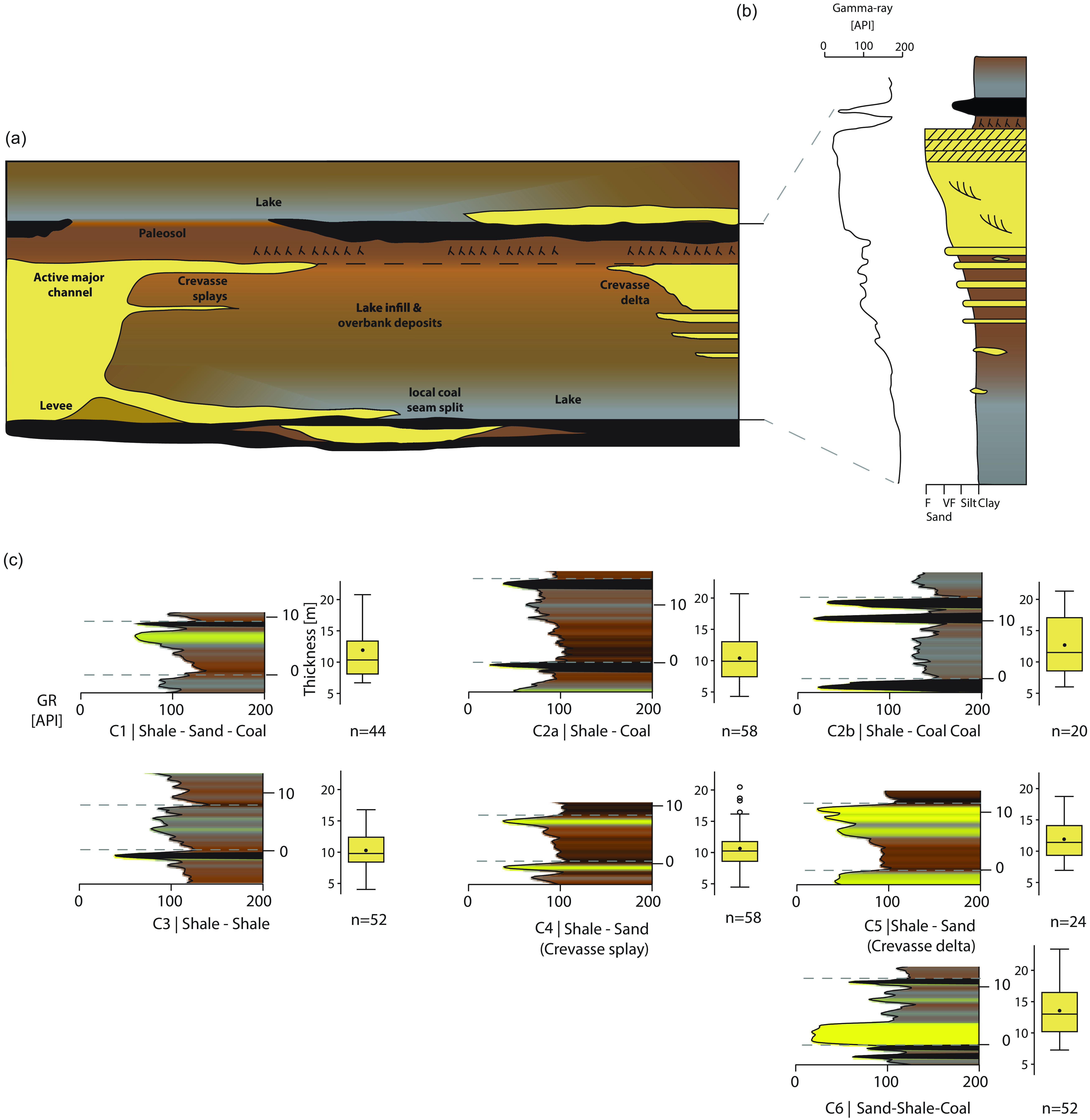
Figure 4. Cyclothems for the Southern North Sea Westphalian. (a) A schematic drawing of facies recognised in the cyclothems with lateral differences illustrated. (b) An idealised succession showing a gradual coarsening-upwards and then rapid fining-upward package moving from fine lake deposits followed by crevasse splay or crevasse delta progradation and subsequently floodplain deposits that are often organic-rich. The rapid upwards fining represents the drowning of the delta top by lake deposits under relative base-level rise (after O’Mara and Turner, Reference O’Mara and Turner1999). (c) Different types of cyclothems defined in this study and their corresponding thicknesses. Type C1 is defined as the ideal cyclothem. Note how a component is absent in each other type defined—for example, the coal in types C3, C4, and C5. See Fig. 3 for the key to the colour fill of the gamma-ray.
Table 1. Cyclothem types (See Fig. 4) and their thickness, variability, and occurrence.

Individual cyclothem thicknesses range from 3.7 m to 22.2 m (mean 11.0 m; median: 10.1 m; SD: 3.8 m; skewness: 0.75; Fig. 5a). There is no significant difference in thickness between most cycle types, other than those with sandstones at the base (type C6), which on average are thicker than the other types (t-test, p < 0.01). The vertical succession of cycle types changes quickly with no dominant successive pattern. The vertical variation in consecutive cycle thickness is reduced to 15% of the mean within five cycles (9.35–12.65 m; Fig. 5c). Cycles in the wells of Transect Two to the northeast are thinner (mean 8.9 m) than those of Transect One to the south and southwest (mean 11.2 m; Fig. 5b).

Figure 5. Cycle thickness statistics. (a) Box plots illustrating the thicknesses of the first 24 correlated cycles and the total thickness based on 311 measurements. Cycle 25 has been excluded as it has only been identified twice. Black dots illustrate the mean thickness for each cycle. Dashed grey lines represent the mean and standard deviation of the total dataset. (b) Plan view of the well’s mean cycle thickness and interpolated thickness contours. Note how the cycle thickness is smaller in transect Two in the north of the study area. (c) The coefficient of variance, an indication for the compensational stacking, is calculated for consecutive cycles over all wells and implies stable thickness variation (15%) near 2–5 cycles.
Sandstone character
A total of 99 sandstones have been documented in this study (Fig. 6a). Most have a blocky pattern (n = 61) with fewer coarsening- and fining-upward sandstones (n = 23 and n = 15, respectively). Blocky pattern sandstones can occur as stacked units of up to four storeys, reaching a cumulative thickness of up to 30 m. They show a bimodal thickness distribution (Fig. 6b) with often single-story, isolated sandstones with a range of 3–6 m and stacked sandstones ranging from 8 to 12 m. The latter often have subtly serrated gamma-ray profiles, while the thinner blocky-pattern sandstones are described as more convex. Both the blocky pattern and fining-upwards sandstones tend to be thicker than the coarsening-upward sandstones (t-test, p < 0.01) which have a mean thickness of 4.3 m (Fig. 6a). Coarsening-upward trends are often seen in sands that are less than 3 m thick, but which are excluded from this study (Figs. 7 and 8). Net-to-gross ratios over all the studied wells are generally low, averaging 13% (min: 5%, max: 22%).

Figure 6. (a) The measured thickness for sandstones >3 m. Based on the log shapes, the sandstones have been divided into three groups: block pattern, coarsening upwards, and fining upwards shapes. (b) Histogram of the block pattern-shaped sandstones. Note the bimodal distribution of the sandstones with 3–6 m block patterns and the thicker, more serrated sandstones.
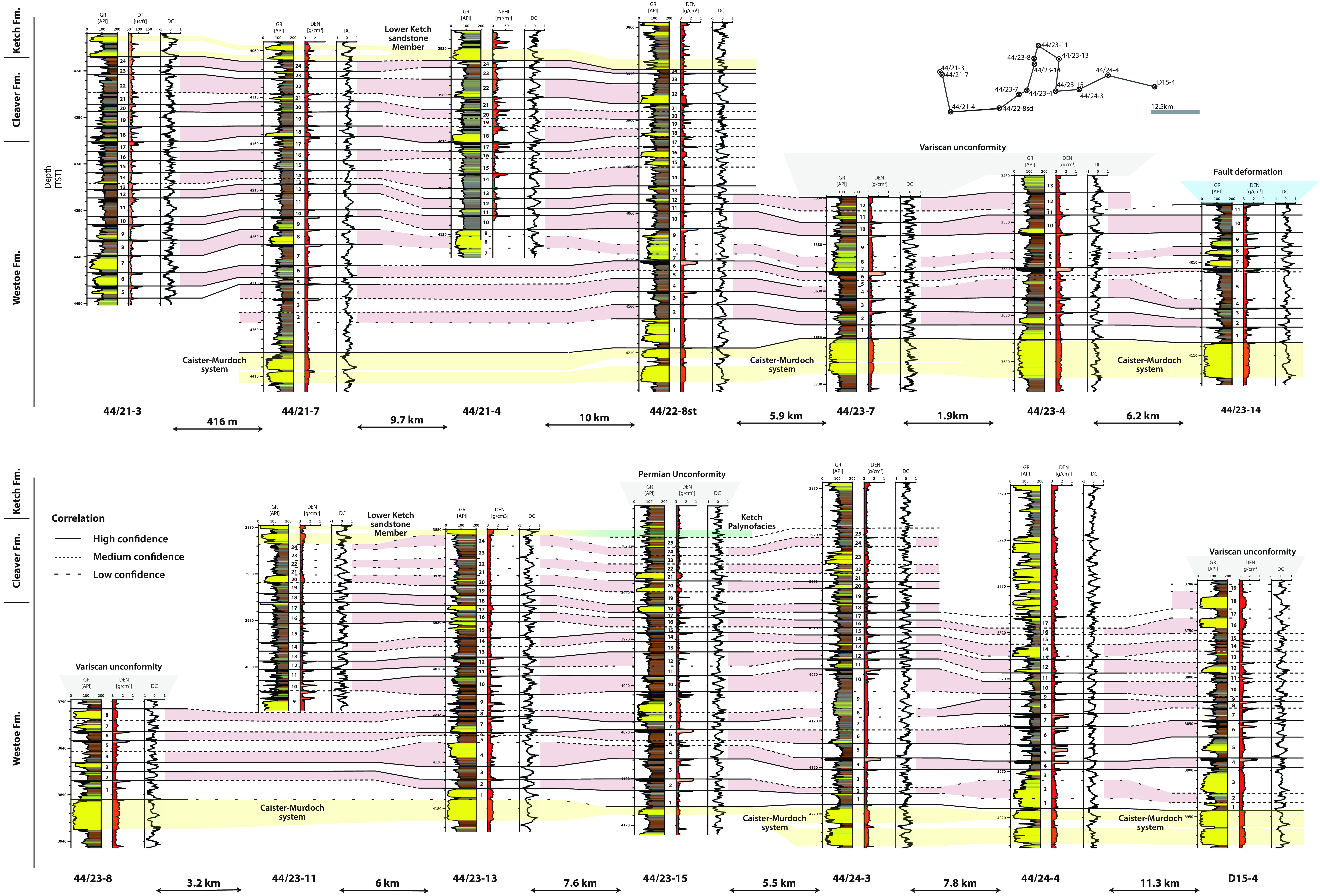
Figure 7. The constructed cyclostratigraphic well correlation of Transect One. The gamma-ray, density and DC records are shown. See Fig. 3 for the key to the colour fill of the gamma-ray. Correlation lines are depicted with three confidence levels (high, medium, and low). Caister-Murdoch system and the Lower Ketch sandstone Member are highlighted in yellow. Grey indicates the Variscan unconformity. The figure is provided in high resolution and can be zoomed in.

Figure 8. The constructed cyclostratigraphic well correlation of the Westoe and Cleaver formations for Transect Two. The gamma-ray, density and DC records are shown. See Fig. 3 for the key to the colour fill of the gamma-ray. Correlation lines are depicted with three confidence levels (high, medium, and low). The Caister-Murdoch system and the Lower Ketch Member are highlighted in yellow. The figure is provided in high resolution and can be zoomed in.
Cyclothem correlation
Manual correlation
The wells were first aligned based on miospore biozones and characteristic lithological patterns. The proximity of the wells allowed for high confidence in correlating lithostratigraphic patterns. The correlation started with three well clusters: 44/21-3, 44/21-7 (416 m), 44/23-8, 44/23-14 (1300 m); and 44/23-4, 44/23-7 (1900 m) and allowed the identification of a marker in the form of a thick coal seam overlain by a thicker sandstone package. This correlates with the top of biozone W4a (Cycle 6). More wells with increasing well spacing up to 12 km, were added using this marker or biostratigraphy. The resulting correlation panels are shown in Figs 7 and 8.
The biostratigraphic zonation and the constructed cyclostratigraphic correlation are generally in agreement (Fig. 9), particularly given the margins for error imparted to the biostratigraphic interpretations by sample distribution. The tops of biozones W4a, W4c, and W5a show a maximum offset of two cyclothems. The top of biozone W4b shows up to 3 cyclothems of offset. In well 44/23-13 the identification the top of the biozone is probably artificial (but would otherwise have an offset of five cyclothems), with the true top lost to erosion Variscan unconformity. The top of the biozone is defined by the top of the common occurrence of Lycospora noctuina noctuina. Any variation in records of this may reflect additional taphonomic controls on species abundance ranges (as compared to species total ranges) which may be exacerbated by practical factors such as the nature and distribution of ditch cuttings samples (e.g. McLean & Davies, Reference McLean and Davies1999). The last occurrence of the L. noctuina noctuina provides a more consistent correlation with the cyclostratigraphic zonation. Accurate recognition of this biostratigraphic event is limited by the scarcity of the species at the limit of its range, meaning that in some cases this event may be artificially deep.

Figure 9. Comparison of biostratigraphic and cyclostratigraphic correlations. Wells are plotted on a composite stratigraphic thickness based on the cyclothem correlation. The green overlay represents the biostratigraphic sampling uncertainty.
Semi-automatic and stratigraphic thickness correlation
A bandpass filter from 8 to 16 m was used to filter the cyclothems from the DC. The semi-automatic correlation was calculated twice. Once using the prominent marker coal seam as a calibration point (Fig. 10b) and once using the top of the Caister-Murdoch system (Fig. 10c). The prominent coal seam was used as a calibration point for correlation based on stratigraphic thickness (Fig. 10d).

Figure 10. Comparison of vertical proportion curves based on different stratigraphic correlation methods. The facies have been divided into sandstone, coal, siltstone, and claystone. The lithofacies distribution has been calculated on a 1 m vertical spacing. (a) Vertical proportion curve based on the manual correlation of cyclothems (see Figs. 7 and 8). (b) Vertical proportion curve based on semi-automatic correlation method of cyclothems with a prominent coal seam a tie-point. (c) Vertical proportion curve based on the correlation of the semi-automatic correlation method with the top of the Caister-Murdoch system as a tie-point. (d) Vertical proportion curve based on true stratigraphic thickness (TST) with a prominent coal seam as a tie-point but without further correlation between wells. Notice how both b, c and d indicate the increase of sand content near the calibration horizon. This zone is similar to the manual correlation. Clay and sand content intervals are well defined in the semi-automatic method (b and c), while this is less prominent in the manual method (a). The vertical grey arrow indicates the 30% level.
Individual cyclothems identified by this correlation are similar to and as well-defined as those identified manually. However, the stratigraphic positions of the cycle boundaries are different. This reflects a slight offset between the wireline data and the resulting DC, resulting in the boundary of a cycle being placed slightly above or below the manually defined boundary (Fig 3c). In thicker sandstones (>10 m), the DC filter detects spectral change in sandstone shape. These changes are included in the automatic correlation, whereas they were treated as unknown intervals and were not used in the manual correlation.
Resulting stratigraphy
Manual correlation
Twenty-five cycles are correlated over an average of 260 m of strata. Cycle thickness and thickness variability is higher in the lowest ten cyclothems (mean: 11.8; SD: 4.4) compared to those above (mean: 10.6; SD: 3.3) (Fig. 5a). Confidence scores are high up to cyclothems 16 or 17. After that, the scores decrease gradually towards the top of the correlation where individual sandstones tend to be more numerous. Coal seams are abundant in the first 16 cyclothems, above which they become less common, especially in the northern part of the study area. It is only in the most southwesterly part of the study area that coals remain common in the higher parts of the sections.
The top of the correlation varies from cycle 23 up to cycle 25. In Transect One, most wells have a thicker sandstone interval on top of cycle 24. Above this interval the sandstone content becomes too dominant for further correlation. This event at the top of cycle 25 is interpreted as the base of the lower Ketch Member. This sandstone interval is absent in wells 44/23-15 and 44/24-3. Here the base Ketch palynofacies is used as a top marker resulting in one cycle offset (cycle 25). In well 44/24-4, no clear top is identifiable. The thick packages of concentrated sandstone from cycle 17 upwards in this well make cyclothem correlation impossible. This sandstone package may represent the local, deep incision by the lower Ketch Member (7 cycles, ± 77 m) although this seems unlikely, given the constant thicknesses of this interval over all of the other wells. It is also possible the section is faulted, causing an offset in correlation. Twenty-three cycles are correlated in Transect Two. The sandstone content becomes too dominant for further correlation above cycle 23 and this interval is interpreted as the lower Ketch Member.
The base of the correlation generally aligns with a thicker sandstone interval, identified as the Caister-Murdoch system. In 44/22-8st, 44/23-4, 44/23-13, and 44/24-4 there is another sandstone on top of the Caister-Murdoch system. There is clear separation between the sandstones with occasional development of coal and so the higher sandstones are interpreted as separate channels above Caister-Murdoch system.
Two intervals of increased sandstone content are identified (Fig 10a). The first (in cycles 7, 8, 9) is of sandstone, c. 30 m thick, that is relatively constant laterally. It often contains multi-story (2–3 stacked) blocky-pattern sandstones where net-to-gross ratios are up to 30–40% (compared to 10–15% elsewhere). The base of the interval is marked by a relatively thick and laterally consistent coal seam forming the top of cycle 6. This coal is probably equivalent to the informal "Coal B" in legacy industry reports. The second interval (cyclothems 17, 18) is c. 20 m thick with an average net-to-gross of 10–15% up to 40%. Here, the sandstone bodies are often thin (<6 m) and single-story, separated by floodplain fines. Between these two intervals (cyclothems 10 to 16), there is an abundance of coal seams and fewer sandstones, which are predominantly coarsening upwards. A general increase in sandstone content characterises the interval above cyclothem 19. However, thick block pattern styled sandstones remain relatively scarce until cycles 23 to 24 and the interpreted base of the lower Ketch Member.
Combination of the vertical proportion curve with the biozonation allows location of marine bands in the cyclostratigraphic framework. The Maltby MB should lie between the top of L. noctuina noctuina and the top of common L. noctuina noctuina (McLean et al., Reference McLean, Owens and Neves2005). Based on the average stratigraphy, the horizon of the Maltby MB is placed at the boundary between cyclothems 16 and 17. Here, the most southerly wells closest to the basin depocentre (44/21-3, 44/21-7, 44/21-4, 44/22-8st) have high gamma-ray values. The horizon of the Aegiranum MB is placed between cyclothems 23 and 24. An evident increase in high gamma-ray values is observed in multiple wells (44/21-3, 44/21-7, 44/21-4, 44/22-8sd, 44/23-15, 44/24-3, 44/23-13). Davies and McLean (Reference Davies and McLean1996) and O’Mara and Turner (Reference O’Mara and Turner1997) suggest that gamma-ray spectrometry can provide a proxy record for marine bands by enhancement in uranium-thorium ratios. Such signals were not identified close to the suggested marine band horizons or at any other depths.
Semi-automatic and stratigraphic thickness correlation
Twenty-six cyclothems are defined in both of the semi-automatic methods, one more than in the manual correlation. In the semi-automatic correlation, some wells appear shifted one cycle up or down compared to the manual correlation. A cyclic character is more clearly visible when comparing the vertical proportion curves of either of the semi-automated correlations than in the manual correlation (Fig. 10b and c). Individual coal seams appear less well-aligned in the semi-automated correlations and sandstones appear to have less stratigraphic overlap, and there are up to 20% higher net-to-gross averages. Both correlations suggest the same large-scale trends in sandstone distribution as the manual correlation, with two intervals of increased net-to-gross. As an independent calculation, the alignment of wells depth based on the true stratigraphic thickness shows a strong smoothing of all facies patterns, particularly at the cyclothem scale of 10–20 m.
Cyclothem duration
The interval between the Vanderbeckei MB and the Aegiranum MB (representing the Duckmantian Substage, Fig. 1b), as defined in the manual correlation, has been used to estimate the duration of a single cyclothem. This interval compromises twenty-three cyclothems, plus the Caister-Murdoch system. The study wells indicate an average additional thickness of 60 m between the base of the Vanderbeckei MB and the top of the Caister Murdoch sandstone. Linear interpolation between the thickness of this interval and the average cyclothem thickness for the remainder of the Duckmantian suggests that it includes five or six additional cyclothems. This implies the presence of twenty-eight or twenty-nine cyclothems in the Duckmantian in the study area. With Duckmantian duration estimates ranging from 1.2 to 2.5 Myr, an individual cyclothem represents a period of between 41 kyr (1.2 Myr, 29 cyclothems) and 89 kyr (2.5 Myr, 28 cyclothems).
Discussion
North Sea Cyclothems
The term cyclothem describes an upward coarsening sequence of claystone to sandstone capped by coal (O’Mara & Turner, Reference O’Mara and Turner1999). Most cyclothems, in the study wells lack some components of the complete cyclothem and different types of cyclothems have been defined accordingly. The most common cyclothem type is a coarsening-upwards shale capped by a coal, differing from the idealised sequence in the absence of sandstone in the top of the sequence. The common denominator of the cyclothems in the Westphalian of the Silverpit Basin is a coarsening upward sequence. A cyclothem containing all lithological elements (type C1) is the ideal or composite cyclothem, while the modal cyclothem is a sequence from shale to coal (cycle type C2a and C2b).
Differences in lithological character and thicknesses of cyclothems reflect local depositional geomorphology, which varied considerably. This is interpreted as an autogenic factor (Fig. 4a). While the geographical extent of ‘minor’ or crevasse deltas and coal mires can be substantial, their lateral continuity is unlikely to extend over tens of kilometres (Haszeldine, Reference Haszeldine1983; Fielding, Reference Fielding1984a; Fielding, Reference Fielding1984b). It should not be expected that the infill of a crevasse delta in a lake would result in a clear gamma-ray signal over a wide lateral distance. Such a feature would only cause a minor change in the gamma-ray trend when observed distal to the sediment source. Peat formation is also expected to occur at a distance from the sediment source (Ferm & Weisenfluh, Reference Ferm and Weisenfluh1989; O’Mara & Turner, Reference O’Mara and Turner1999). Furthermore, autogenic processes such as differential compaction and channel switching can affect the lateral character of a cyclothem.
The documented thicknesses of the cyclothems are comparable to those reported by O’Mara and Turner (Reference O’Mara and Turner1999). Duff and Walton (Reference Duff and Walton1962) observed cyclothems with a similar thickness range of 4 to 20 m (average 11.5 m) in the Pennine Basin. They also recorded variations in cyclothem character, documenting a dominant coarsening upward sequence with the occasional absence of siltstones, sandstones, or palaeosols, similar to that seen in the present study. Further South, in the Dutch onshore on the other side of the Silverpit Basin depocentre, van der Belt et al. (Reference van den Belt, van Hoof and Pagnier2015) documented cyclothems ranging from 5 to 35 m with an average of 12.5 m. The continuous vertical and lateral detection of cyclothems in the study area and similar observations in other parts of the basin suggests a strong, basin-wide, allogenic forcing on deposition.
Sandstone type and occurrence
Wireline data alone does not provide enough evidence to allow interpretation of fluvial formation processes of the three major sandstone types, but it can be linked to outcrop analogues in the Pennine Basin. Fielding (Reference Fielding1984b, Reference Fielding1986) described major and minor distributary channels in the Westphalian. Major distributary channels are broad, elongate, laterally extensive sandstone bodies with low sinuosity and widths of 2–10 km (Fielding, Reference Fielding1984b). Belts of such channels could be linked to the thicker block-shaped sandstones documented on wireline data in this study (Fig. 6). The stacking nature of these sandstone types is documented onshore. The thinner, more convex-shaped, block patterned sandstones can be interpreted as major crevasse channels. These coarse-grained deposits have a maximum thickness of 7 m and a lateral extent of roughly 2 km. Notably, the sharp boundary at the top of the sandstones suggests rapid channel abandonment. Fielding (Reference Fielding1986) argues that such crevasse channels were active for prolonged periods and could transform into minor distributary channels. In contrast, he attributed sandstones with a fining-upward profile to high sinuosity channels. These are like the fining-upward sandstones documented in the present study. However, such channels in the Silverpit area are significantly thicker (up to 12 m) than the 6 m recorded by Fielding (Reference Fielding1986). Sandstones with a coarsening-upward wireline profile most likely represent crevasse delta splays. The pronounced shape relates to the progradation of a crevasse delta into a lake or floodplain. Such overbank deposits have a limited lateral extent of a few hundred meters (Fielding, Reference Fielding1984b). Besides the documented thick (>3 m) sandstones, there are thin (0.5–2 m) single crevasse splays attributed to cycle type C4. The lateral extent of these crevasse splay sandstones is believed to be considerable, but they vary in thickness (Fielding, Reference Fielding1984b).
Manual cyclothem correlation
Neither coal seams nor crevasse delta or splay deposits can be correlated one-to-one between wells. The correlation here was not based on lithologies but on trends. Part of the ability to recognise cyclothem trends and correlate despite lateral character changes is attributed to the use of the DC. With this curve, changes in the wireline record become less dependent on absolute values. While absolute values may change laterally and vertically, the DC filter depicts these changes as equal, allowing cyclic signal detection, as illustrated by the semi-automatic vertical proportion curves (Fig. 10b and c). Further, when attempting a correlation exercise, it is essential to start in neighbouring wells where lateral changes are least, and confidence in correlation is highest. Information about lateral variations in lithofacies in these closely-spaced wells can be used as feedback when making correlations over greater distances.
Even with an understanding of the variability in the system, part of the correlation remains uncertain. This is often highest around thicker channel sandstones, where the preservation potential of cyclothems is lowest. Below channel sand bodies there may be gaps in the stratigraphical record due to incision. In the Pennine Basin, the maximum erosional relief of the major channels during the Westphalian is estimated at 6–10 m of compacted stratigraphy (Fielding, Reference Fielding1986). In the study area the Caister-Murdoch system has erosional relief of up to 15 m (O’Mara & Turner, Reference O’Mara and Turner1999). Sandstones frequently occur directly on top of coal seams. Primary compaction of coals (up to 47% of the total compaction) occurs rapidly, with average compaction rates of 5–24 mm/yr (Cahoon et al., Reference Cahoon, Marin, Black and Lynch2000; Törnqvist et al., Reference Törnqvist, Wallace, Storms, Wallinga, Van Dam, Blaauw and Snijders2008; van Asselen et al., Reference van Asselen, Stouthamer, van and Th2009). Such early lithification may suggest that even relatively young, buried peats could act as barriers to channel incision. Given this and the low relief of the Westphalian alluvial plain, it seems unlikely that channels could have removed more than two full cyclothems by incision. To address these issues intervals with thick sandstone bodies are scored with lower certainty than adjacent intervals. This results in a lower stratigraphic resolution for the sandstone-prone sections. However, the adjacent intervals (being constrained by biostratigraphic and lithostratigraphic markers) have higher certainty and so any stratigraphical gaps associated with sandstone incision do not represent problems for cyclothem correlation.
Resulting stratigraphy
There is a clear difference between the average cyclothem thickness in the southern (Transect One, 11.2 m) and northern (Transect Two, 8.9 m) transects. This reflects the southwestward increase in overall stratal thickness towards the basin depocentre. The change occurs over a relatively short distance of about 10 km. The orientation of the thickness change is perpendicular to a dominant northwest-southeast fault trend observed in the Silverpit Basin, thought to be related to the approaching Variscan deformation from the south (Leeder & Hardman, Reference Leeder and Hardman1990). This may be an extension of the Elbe-Odra fault line (Smit et al., Reference Smit, Wees and Cloetingh2016) and may have been a hinge line that created more accommodation space on its south-southwest side. Alternatively, compartmentalisation of the foreland basin into small fault blocks with varying subsidence and accommodation space may account for the thickness changes. A similar feature is described for the Oligocene Boom Clay in the Campine area, Belgium where bed-to-bed correlations provided evidence differential subsidence of closely spaced fault blocks (Vandenberghe & Mertens, Reference Vandenberghe and Mertens2013).
The base of the correlation is bounded by the Caister-Murdoch system, and based on the cyclostratigraphic correlation, this lithological unit’s position remains consistent. The position of the base of the lower Ketch Member differs being defined one cycle earlier in the Northeast (Transect Two). As with the change in cyclothem thicknesses, the overall study interval is thinner, in the Northeast. This is in line with the general northeast thinning trend of the Westoe and Cleaver formations (Huis in ‘t Veld et al., Reference Huis in’t Veld, Schrijver and Salzwedel2020) and may reflect differences in accommodation space, with a larger sub-Ketch disconformity towards the north and consequent lower preservation potential in the upper part of the study interval.
Cyclostratigraphy compared to biostratigraphy
There is an average offset of 1–3 cyclothems or roughly 10–30 m between the biostratigraphy and the cyclostratigraphic framework. Several practical and geological factors impart margins of error on the use of miospores in the study. These include: sample density varies within and between the wells; all samples are from ditch cuttings that allow a maximum stratigraphical resolution of 3 m; the scarcity of species at the stratigraphical limits to their ranges can lead to false-negative results in the correct identification of a biostratigraphical event (species inception of extinction); and miospores are generally absent in medium- to coarse-grained clastics. Further, as different lithologies and facies provide different miospore assemblages (Neves, Reference Neves1958) the stratigraphical ranges of many species in coal seam samples appear shorter than in clastic samples (McLean et al., Reference McLean, Owens and Neves2005).
Semi-automated and stratigraphic thickness correlation
The semi-automatic and manual correlations are closely comparable. Individual cyclothems are often similarly defined, but cyclothem boundaries may be slightly offset. This is probably caused by a small "lag effect" of the DC on the wireline data and the use of a bandpass filter to smooth the signal (Fig. 3c) which may result in the misalignment of coal seam signals. However, the vertical proportion curves of the semi-automatic correlation (Fig. 10b and c) have a more distinctly cyclical pattern, reflecting the dominant influence of sandstones in the DC. The vertical proportion curves of the semi-automatic correlation result in apparent thinning of sandstone intervals and 20% higher net-to-gross ratios. They detect and suggest intervals of alternating sandstones and fine-grained clastics resulting in apparently low stratigraphic overlap of sandstones and laterally extensive, fine-grained clastics. These fine-grained intervals may act as flow barriers in a reservoir. When autogenic variability is taken into account, the manual correlation results in a model with more stratigraphic overlap of sandstones and suggests greater vertical sandstone connectivity. However, with its ease of use and faster output when looking at implementation into subsurface workflows and basin-wide trends, the benefits of the semi-automated method may outweigh the cost of any resultant uncertainties.
Using an equal thickness assumption, the calculated stratigraphic thickness correlation results in smoothed facies patterns. These are particularly evident at cyclothem scales of 10–20 m. Large-scale trends remain recognisable which is probably related to compensational stacking patterns within the system. The tendency for sediment transport systems to preferentially fill topographic lows produces an averaged equal thickness (Straub et al., Reference Straub, Paola, Mohrig, Wolinsky and George2009). Within two to five cycles (22–55 m), the average stacked thickness of cyclothems varies only by 1.65 m. Any patterns above this resolution appear to remain equal.
Controls on sedimentation
A depositional model driven by glacio-eustatic, base-level change explains the deposition of the cyclothems in the Silverpit Basin. Each cyclothem has a fine-grained, lacustrine, or marine bed at its base representing a (forth-order) base-level high-stand. Lacustrine or marine accommodation space is subsequently filled base-level fall (O’Mara & Turner, Reference O’Mara and Turner1999; Huis in ‘t Veld et al., Reference Huis in’t Veld, Schrijver and Salzwedel2020). However, glacio-eustasy will also have effected changes upstream. Palaeo-polar ice volume changes are also related to palaeo-tropical climatic variations with changes in rainfall and vegetation affecting upstream sediment supply and leading to cyclic behaviour in fluvial systems (e.g. Noorbergen et al., Reference Noorbergen, Abels, Hilgen, Robson, de Jong, Dekkers, Krijgsman, Smit, Collinson and Kuiper2018; Opluštil et al., Reference Opluštil, Laurin, Hýlová, Jirásek, Schmitz and Sivek2022). There is strong evidence that Pennsylvanian glacial-interglacial fluctuations produced significant climatic variations, with shifts from perhumid to semi-arid seasonal climates recorded in palaeotropical Euramerica (Cecil et al., Reference Cecil, Dulong, West, Stamm, Wardlaw and Edgar2003; Roscher and Schneider, Reference Roscher and Schneider2006; DiMichele et al., Reference DiMichele, Cecil, Montañez and Falcon-Lang2010; Eros et al., Reference Eros, Montañez, Osleger, Davydov, Nemyrovska, Poletaev and Zhykalyak2012). Cecil et al. (Reference Cecil, Dulong, West, Stamm, Wardlaw and Edgar2003) argue that changes in the position of the intertropical convergence zone caused relatively wet conditions in the palaeotropics during interglacials, while the climate was drier and more seasonal during glacials. Higher interglacial precipitation would stimulate peat development and, ultimately, the extended formation of lakes. Lower precipitation and enhanced seasonality during glacials would have decreased vegetation cover (DiMichele et al., Reference DiMichele, Cecil, Montañez and Falcon-Lang2010; Eros et al., Reference Eros, Montañez, Osleger, Davydov, Nemyrovska, Poletaev and Zhykalyak2012) resulting in higher sediment influx and the infilling of lakes with coarser-grained clastics. With the absence of clear marine conditions in the Westoe Formation (O’Mara & Turner, Reference O’Mara and Turner1997) and probable upstream changes, both upstream and downstream controls, and likely combined, should be considered as mechanisms in the formation of cyclothems in the Silverpit Basin.
Cyclothem duration
The absence of sufficient chronological dating in the Silverpit Basin and the large variability in age control makes it challenging to identify an orbital forcing component in the depositional system. Different time scales, suggest a duration of between 41 and 89 kyr for cyclothem formation. In the Dutch onshore, van der Belt et al. (Reference van den Belt, van Hoof and Pagnier2015) identified cyclothems paced at a sub-eccentricity periodicity with dominant ∼21 kyr precession and interference of an obliquity component. For the central Appalachian Basin, Le Cotonnec et al. (Reference Le Cotonnec, Ventra, Hudson and Moscariello2020) suggested cyclothem forcing by the interference of ∼34 kyr obliquity and ∼100 and ∼400 kyr eccentricity, while for Eastern European Basins a ∼100 kyr short-eccentricity is proposed (e.g. Davydov et al., Reference Davydov, Crowley, Schmitz and Poletaev2010; Jirásek et al., Reference Jirásek, Opluštil, Sivek, Schmitz and Abels2018; Opluštil et al., Reference Opluštil, Laurin, Hýlová, Jirásek, Schmitz and Sivek2022). In the Eastern European Upper Carboniferous, cyclothems are 50 to 100 m thick and commonly include multiple coal sequences. Jirásek et al. (Reference Jirásek, Opluštil, Sivek, Schmitz and Abels2018) suggest the presence of obliquity or precession-controlled patterns on coal seam distribution within these thicker cyclothems.
Coal bundles which might suggest a larger-scale forcing were not observed in this study. However, the two large-scale trends of increased net-to-gross zones are separated by eleven cyclothems. This is also the case between the first interval and the Vanderbeckei MB. The constant spacing and the 11:1 ratio between the intervals are comparable to the ratio of the ∼34 kyr obliquity period during the Carboniferous (Collier et al., Reference Collier, Leeder and Maynard1990) and the ∼400 kyr long-eccentricity cycles. Oligocene sedimentary records also show that glacio-eustasy has a strong obliquity component with long-eccentricity modulation (e.g. Wade and Pälike, Reference Wade and Pälike2004; Abels et al., Reference Abels, Simaeys, Hilgen, Man and Vandenberghe2007). This may suggest that the Silverpit Basin cyclothems had a strong obliquity-controlled component which was shorter than the estimated duration. However, there is a large uncertainty regarding age control. One could also argue for the existence of a ∼100 kyr short-eccentricity control, but a strong imprint of long-eccentricity (4:1 ratio) would be expected, which is not found.
Low net-to-gross targets
The two defined increased net-to-gross intervals, and the Caister-Murdoch system could be paced at a ∼400 kyr long-eccentricity interval (Fig. 11). Long-eccentricity modulation of glacio-eustasy (e.g. Wade and Pälike, Reference Wade and Pälike2004; Abels et al., Reference Abels, Simaeys, Hilgen, Man and Vandenberghe2007) would have led to more extreme base-level fluctuations at specific intervals, and potentially resulting in incised valley fills. The Caister-Murdoch system was formed as an incised valley fill (Shanley and McCabe, Reference Shanley and McCabe1994; Ritchie et al., Reference Ritchie, Pilling and Hayes1998; Huis in ‘t Veld et al., Reference Huis in’t Veld, Schrijver and Salzwedel2020) or due to tectonic influence (O’Mara & Turner, Reference O’Mara and Turner1999; Kosters & Donselaar, Reference Kosters and Donselaar2003). The vertical distribution and spacing of the Caister-Murdoch system, lower Ketch sandstone, and the two newly defined increased net-to-gross intervals suggests that it is unlikely that all of these sandstone-prone intervals were tectonically induced. Therefore, the two defined increased net-to-gross intervals could also represent incised valley fills.
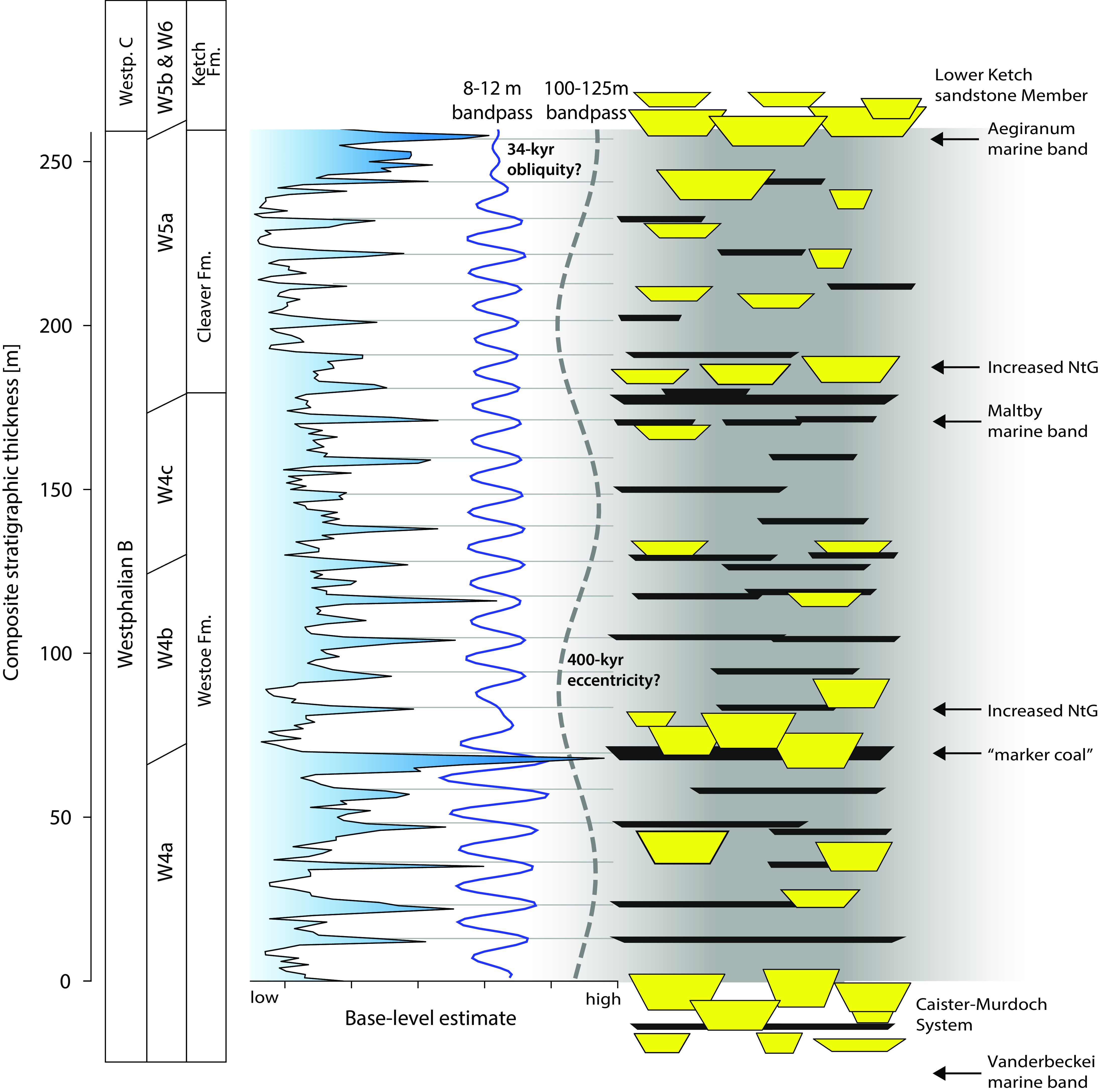
Figure 11. A base-level estimate curve based on the vertical proportions curve of the manual correlation. In blue, an 8–12 m and in grey, a 100–125 m bandpass filter is shown. The Caister-Murdoch sandstones and Ketch sandstones are indicated at the section’s bottom and top, respectively. Based on the average stratigraphic trends, two zones with increased sand lithofacies are defined and shown on the right. These zones align with a 100–125 m bandpass filter and could possibly be controlled by a ∼400 kyr long-eccentricity pacing.
Another explanation for the two-increase net-to-gross intervals can also be given. In the low-relief setting of the Silverpit Basin, a significant lowering of base-level could have changed the fluvial planform style towards the braided end of the alluvial spectrum. Such change is observed in the first low net-to-gross interval, where multi-storied block patterned sandstones are more common. Furthermore, greater extremes in base level fluctuation would also have led to enhancement of upstream sediment flux. This model would fit with the stratigraphical juxtapositioning of prominent coal seam markers and marine bands indicating enhanced wetter periods (Fig. 11).
Independent of the specific depositional model for the defined increased net-to-gross intervals, an orbitally forced control would affect reservoir potential. Basin-wide forcing implies a more significant probability of the occurrence of sandstones within these stratigraphic intervals in the otherwise overall low net-to-gross Westoe and Cleaver Formations. Similar variations in net-to-gross ratios associated with long-eccentricity climate control are suggested for the Upper Carboniferous Upper Silesian (Opluštil et al., Reference Opluštil, Laurin, Hýlová, Jirásek, Schmitz and Sivek2022) and Appalachian Basins (Le Cotonnec et al., Reference Le Cotonnec, Ventra, Hudson and Moscariello2020).
Conclusions
Repetitions of coarsening upward sequences, cyclothems, continuously occur in the Westoe and Cleaver formations in the Silverpit Basin in the Southern North Sea. These can be used for cyclostratigraphic correlation and identification of stratigraphic trends in this low net-to-gross interval. The average cyclothem thickness implies that a high-resolution correlation is possible but to achieve this the variability in thickness and lithological character, interpreted as local, autogenic components, must be considered. Five variations in cyclothem development are defined in relation to an ideal cyclothem consisting of a coarsening upwards sequence of shale to sandstone capped by coal and five variations.
Manual and semi-automated methods for the correlation of wells are evaluated, and average stratigraphic trends are compared. The manual correlation demonstrates that wells can be correlated at a 10–20 m resolution, even over large well spacings. This correlation generally agrees with the available biostratigraphic control. The semi-automated methods uses a deviation curve as an essential technique allowing identification of cyclothems relatively easily. However it is not as accurate as the manual correlation. The vertical proportions curve of the manual correlation indicates a higher level of stratigraphic overlap of sandstone bodies than expected for a fully cyclic-driven model. Similar trends are seen in the vertical proportions curve in the semi-automated method. Here, all sandstones relate to the same stratigraphic level. In the manually derived vertical proportions curve, claystones are stratigraphically more spread and represent fewer potential flow barriers than suggested by the semi-automated correlation. On balance, the ease of use and faster output of the semi-automated method outweighs the uncertainties produced. This is so particularly when looking at basin-wide trends for implementation into subsurface workflows.
Both correlations identify two laterally consistent intervals where net-to-gross increases from 10–15% to 30–40%. The lower interval in the Westoe Formation has the highest reservoir potential of the two. Here the sandstones are commonly stacked, multi-story units. These intervals are interpreted as being linked to a ∼400 kyr long-eccentricity control on base-level fluctuation and associated upstream changes in hydrology. Such an orbitally forced control implies a stratigraphic predictive value. These intervals have a higher probability of sandstone occurrence and their recognition by cyclostratigraphic analysis may guide economic exploration in an otherwise low net-to-gross setting.
Supplementary material
The supplementary material for this article can be found at https://doi.org/10.1017/njg.2023.8.
Acknowledgements
We want to thank Stephan de Hoop for their help with writing the code for part of the analysis conducted in this study. We also want to thank two anonymous reviewers for improving this manuscript. This study was financially supported by Top Sectors GeoEnergie, Wintershall Noordzee B.V. and Equinor ASA (FRESCO Project, Grant Number TKI2018–03–GE). MB Stratigraphy Ltd benefitted from the HMRC R&D Tax credit SME scheme. The authors do not have any conflicts of interest.


 Open access