


Introduction
Sediments preserve specific characteristics for each depositional environment. As these alter through time, a succession of sediment facies is generated. Each of them is defined as the sum of a sedimentary unit’s primary characteristics with possible diagenetic alterations (Reineck & Singh, Reference Reineck and Singh1986). As a result, classifying sediment records into sediment facies is vital for studying palaeoenvironmental variability, climatic variation, archaeological aspects and natural resource potentials. For instance, lake-level fluctuations identified by sediment facies changes in the Dead Sea indicate climatic variation (Ben Dor et al., Reference Ben Dor, Neugebauer, Enzel, Schwab, Tjallingii, Erel and Brauer2019). Sometimes climatic variation is accompanied by adaptation of human settlements (e.g. Behre, Reference Behre2004). In addition to palaeoenvironmental reconstruction, geochemical proxies measured in sediments are useful to depict climatic variation but need to be interpreted carefully including background knowledge of respective sediment facies (Davies et al., Reference Davies, Lamb and Roberts2015; Rothwell & Croudace, Reference Rothwell, Croudace, Croudace and Rothwell2015). Also the detection of oil and gas reservoirs relies on lithological facies, especially as their exploration is coming to an end (Ai et al., Reference Ai, Wang and Sun2019). Thus, discrimination of sediment facies and stratigraphic units needs to be observer-independent and cost-efficient to cope with such an abundance of applications.
The conventional approach of facies discrimination is mainly based on classical core description. Macroscopically and/or microscopically determined sediment structures and colours combined with basic physical, chemical and biological information, such as the hydrochloric acid (HCl) test for carbonates, and smear slides for identifying minerals and organisms (e.g. diatoms and foraminifers) are used to distinguish different sediment facies (Anderton, Reference Anderton1985; Flügel, Reference Flügel2010; Daidu et al., Reference Daidu, Yuan and Min2013; Bulian et al., Reference Bulian, Enters, Schlütz, Scheder, Blume, Zolitschka and Bittmann2019). This description is a qualitative measure relying on the experience of scientists. To increase observer-independent measurements that can be effortlessly reanalysed or adopted by further studies, quantitative laboratory measurements such as grain size, bulk geochemical and faunistic analyses need to be carried out. However, these quantitative methods are usually time-consuming, labour- and cost-intensive as well as challenging for achieving high-resolution measurements.
The development of rapid high-resolution and non-destructive down-core scanning techniques has improved the situation for physical and chemical sediment parameters recently. For instance, X-ray fluorescence (XRF) core scanners offer elemental profiles with up to 100 μm down-core resolution and digital images with a maximum resolution of less than 50 μm per pixel (Croudace et al., Reference Croudace, Rindby and Rothwell2006, Reference Croudace, Löwemark, Tjallingii and Zolitschka2019). Additionally, computed tomography (CT) scanning provides 3D radiographic images with up to 40 μm per voxel (volumetric pixel; Geotek Ltd, 2018) and density-related values in Hounsfield units (HU) (Hounsfield, Reference Hounsfield1973) after calibration. At a considerably lower spatial resolution of 4 mm, magnetic susceptibility (MS) profiles provide information about the content of iron-bearing (magnetic) minerals (Zolitschka et al., Reference Zolitschka, Mingram, Van der Gaast, Jansen, Naumann, Last and Smol2001). Data acquisition for all these techniques can take place within hours for a c.1 m long core section. Combining these scanning parameters provides a digital alternative for thoroughly describing sedimentary records (semi-)quantitatively. These data compare well with other studies and use less time and labour with reference to quantitative methods relying on individual samples.
Our study area is the shallow coast of northwestern Germany with its high variability along the North Sea Basin (Streif, Reference Streif2004). This region has undergone rapid changes since the sea-level low stand during the Last Glacial Maximum, when the coastline was shifted southward by >800 km. With the rising sea level (Vos & Van Kesteren, Reference Vos and Van Kesteren2000; Meijles et al., Reference Meijles, Kiden, Streurman, Van der Plicht, Vos, Gehrels and Kopp2018), the environment changed from terrestrial (glacial moraines, eolian, fluvial, peat) via intertidal to shallow marine (Behre, Reference Behre2004; Streif, Reference Streif2004), where barrier islands, lagoons, tidal flats and channels as well as marsh environments were formed (Dijkema et al., Reference Dijkema, Reineck, Wolff and Group1980; Ehlers, Reference Ehlers1988). Consequently, many different facies are preserved in the sediment records, all of which provide an excellent opportunity for testing down-core scanning techniques for a (semi-)quantitative facies description.
Several studies investigated sediments from the Wadden Sea. Some used conventional geochemical methods, such as elemental analyses, and grain-size analysis of discrete samples, to discuss sediment dynamics in salt marsh, lagoonal and tidal-flat environments (Dellwig et al., Reference Dellwig, Hinrichs, Hild and Brumsack2000; Kolditz et al., Reference Kolditz, Dellwig, Barkowski, Badewien, Freund and Brumsack2012a,b). Element ratios are often applied in these studies, such as the Ca/Sr and Zr/Al ratios, to characterise the sediment. Some studies integrate palaeontological analyses to discover more details with regard to climatic oscillations and depositional evolution (Dellwig et al., Reference Dellwig, Gramberg, Vetter, Watermann, Barckhausen, Brumsack, Gerdes, Liebezeit, Rullkötter, Scholz-Böttcher and Streif1998, Reference Dellwig, Watermann, Brumsack and Gerdes1999; Freund et al., Reference Freund, Gerdes, Streif, Dellwig and Watermann2004; Schüttenhelm & Laban, Reference Schüttenhelm and Laban2005; Beck et al., Reference Beck, Riedel, Graue, Köster, Kowalski, Wu, Wegener, Lipsewers, Freund, Böttcher, Brumsack, Cypionka, Rullkötter and Engelen2011; Bulian et al., Reference Bulian, Enters, Schlütz, Scheder, Blume, Zolitschka and Bittmann2019). Since peats play an essential role in this coastal region, some studies focus on its formation’s chemical and biological processes (e.g. Dellwig et al., Reference Dellwig, Böttcher, Lipinski and Brumsack2002). Furthermore, several studies stress that anthropogenic influences like land reclamation, dredging, dike building, and harbour activities in recent times are causing a loss of fine-grained sediments (Flemming & Nyandwi, Reference Flemming and Nyandwi1994; Flemming & Ziegler, Reference Flemming and Ziegler1995; Dellwig et al., Reference Dellwig, Hinrichs, Hild and Brumsack2000; Hinrichs et al., Reference Hinrichs, Dellwig and Brumsack2002).
This study combines measurements from four scanning techniques (MS, CT, µ-XRF, digital photography) to digitally characterise different facies and compare results with qualitative lithological descriptions. It aims at evaluating the potential of high-resolution physical and chemical measurements provided by down-core scanning techniques as a means of reproducing sedimentological observations in a digital perspective. We want to test whether scanning parameters and facies determined by macroscopical observations differ and if this information can later be used for automatic facies discrimination.
Methods and materials
Coring
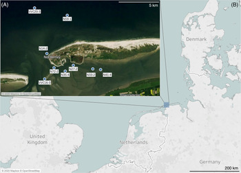
Our study area is located in the East Frisian Wadden Sea near the island of Norderney, Germany, at the southern margin of the North Sea shelf (Fig. 1). More than 140 sediment cores (length: up to 6 m, diameter: 8 and 10 cm) were recovered in the framework of the interdisciplinary Wadden Sea Archive (WASA) project from tidal flats, channels and offshore (Fig. 1). The cores were drilled using a Vibracorer (VKG-6), cut into ˜1 m-long sections and stored at +4°C in the core repository of the GEOPOLAR lab, University of Bremen, Germany. For this study, 10 core sections up to 1.2 m long were selected (Fig. 1; Table S1 (in the supplementary material available online at https://doi.org/10.1017/njg.2021.6) with basic information). These contain a representative selection of all major sediment facies retrieved up to the start of this study.

Fig. 1. (A) Island of Norderney and sampling positions of analysed sediment core sections. Sections VVC16-3 and VVC16-4 belong to the same position. (B) Regional base map. The maps were captured from OpenStreetMap (https://www.openstreetmap.org/copyright).
Lithology description
The sediment cores were split lengthwise using a metal wire, and sedimentary facies were described macroscopically. This description includes visible sediment structures, grain size, colour, carbonate content and biological remains. Occasionally, smear slides were made and selected sediment components were microscopically identified.
Down-core scanning techniques
The sediment surfaces of working halves were carefully cleaned with a razor blade prior to scanning. Core faces were covered by wrapping film during MS and CT scanning but not during µ-XRF scanning and digital photography. Measurements were taken exclusively in the centre of the core to avoid possible coring artefacts (e.g. bending of layers) caused by the coring technique.
Magnetic susceptibility
The split-core surface’s magnetic susceptibility was scanned in 1 cm increments using a Bartington MS2F point sensor at the GEOPOLAR lab (Zolitschka et al., Reference Zolitschka, Mingram, Van der Gaast, Jansen, Naumann, Last and Smol2001). The sensitive volume of the probe is 15 mm (diameter) × 6 mm (depth) (Dearing, Reference Dearing1999).
X-ray density
The split-core halves of the sediment sections were scanned with a Toshiba Aquilion 64 computed tomography (CT) with 0.35 × 0.35 × 0.5 mm3 (x, y, z-direction) resolution at the hospital Klinikum Bremen-Mitte. The scanner used a voltage of 120 kV and a current of 600 mA as X-ray source parameters. Obtained X-ray topograms were reconstructed with Toshiba’s patented helical cone-beam reconstruction technique and an overlapping resolution in z-direction of 0.3 mm. Each voxel provides X-ray attenuation at the given position. X-ray attenuation reflects the object density measured in Hounsfield units (HU), based on a linear calibration of X-ray density with distilled water set to 0 HU and air set to −1000 HU (Hounsfield, Reference Hounsfield1973). X-ray attenuation is additionally influenced by the sediment’s elemental composition (Hounsfield, Reference Hounsfield1973; de Montety et al., Reference de Montety, Long, Desrosiers, Crémer, Locat and Stora2003).
The reconstructed 3D X-ray attenuation (henceforth CT-density) data were analysed using the ZIB edition of the Amira software (version 2019.39; Stalling et al., Reference Stalling, Westerhoff and Hege2005; http://amira.zib.de) to visualise and measure spatial variations of the internal composition. Within Amira and prior to all analyses, the core liners and about 2 mm of the outer core rims were deleted from the data set. Sediment constituents, such as peat, rhizoliths, lithic clasts, shells and the sediment matrix, were separated with a marker-based watershed algorithm, i.e. a Watershed (Skeleton) Module. Markers were set by threshold segmentation within the Segmentation Editor. CT-density values of the combined sediment matrix and peat constituents were determined by mean density per slice using the Material Statistic Module. Other constituents were excluded. To avoid coring artefacts, which are prominent especially at the outer rims of the cores, only values from the core centre (Ø: ∼3.5 cm) were extracted.
Elemental intensities and lightness (L*)
Elemental intensities and digital images were obtained directly from the split-core surfaces using a COX Itrax-XRF core scanner at the GEOPOLAR lab. XRF measurements were taken with a 2 mm down-core scanning step size and a chromium X-ray tube and this setting: 30 kV voltage, 45 mA current and 5 s exposure time. The generated X-ray beam analysed a 20 × 0.2 mm2 wide rectangle with its long axis perpendicular to the core axis. Resulting XRF spectra were evaluated by the Q-Spec software (version 2015; COX Analytical Systems) to calculate elemental peak areas as total counts. Twelve elements (Si, S, Cl, K, Ca, Ti, Fe, Br, Rb, Sr, Zr, Ba) were selected based on the following criteria: (1) the fluorescence signal of the analytes must not be severely affected by the X-ray tube’s primary radiation and has maximum counts >500, and (2) median counts are >100 or coefficients of variance are >2.
We applied a centred log-ratio (clr) transformation on selected element counts to eliminate down-core bias caused by X-ray tube ageing, physical sediment variation and the closed-sum effect (Aitchison, Reference Aitchison1986; Weltje &Tjallingii, Reference Weltje and Tjallingii2008; Lee et al., Reference Lee, Huang, Burr, Kao, Wei and Liou2019). Subsequently, a principal component analysis (PCA) was performed to reduce the data dimension with a minimal loss of variance and highlight major elements’ behaviour (Loska et al., Reference Loska and Wiechuła2003; Schwestermann et al., Reference Schwestermann, Huang, Konzett, Kioka, Wefer, Ikehara, Moernaut, Eglinton and Strasser2020). However, to eliminate sample-size bias and compensate for differences in variance between elements during PCA calculation, (1) the number of data points belonging to each facies needs to be equal, and (2) each element profile needs to be standardised to unit variance and zero mean. Therefore, 500 data points were randomly selected without replacement in each facies that has >500 data points. For facies with fewer data points, 500 data points were randomly selected with replacement. The original data points for each facies are listed in Table S2 (in the supplementary material available online at https://doi.org/10.1017/njg.2021.6). We used the Python package scikit-learn (Pedregosa et al., Reference Pedregosa, Varoquaux, Gramfort, Michel, Thirion, Grisel, Blondel, Prettenhofer, Weiss, Dubourg, Vanderplas, Passos, Cournapeau, Brucher, Perrot and Duchesnay2011) to train the PCA model with this homogenised and standardised data. In the model, the dimensions of elemental intensities were reduced to several principal components (PCs) based on the elbow concept (Fig. S1 in the supplementary material available online at https://doi.org/10.1017/njg.2021.6) and the preference for components having more than 10% of the total variance (Kaiser, Reference Kaiser1960). Subsequently, the model is used to reduce the dimensions on the standardised data without prior homogenisation.
The optical-line camera is equipped with a light-sensitive 2048 pixel CMOS (complementary metal-oxide-semiconductor) device that generates high-resolution digital photographs (47 μm/pixel) of the sediment surface (Croudace et al., Reference Croudace, Rindby and Rothwell2006). These digital images are in 8-bit RGB colour space designed for television and monitors. The colour space was transformed into CIE (Commission Internationale de l’Éclairage) L*a*b* space, which is suited to depict colour variations closer to human perception and commonly accepted by sediment colour studies (Berns, Reference Berns2000; Nederbragt & Thurow, Reference Nederbragt and Thurow2005). The Python package scikit-image (Van der Walt et al., Reference Van der Walt, Schönberger, Nunez-Iglesias, Boulogne, Warner, Yager, Gouillart and Yu2014) conducted the transformation with the most commonly used settings (illuminant: D65, observer: 2) referring the pure white as seen by natural daylight (Nederbragt et al., Reference Nederbragt, Francus, Bollmann and Soreghan2005). L* variations were determined down-core by calculating the average L* value for each depth. All values were extracted from the central area (width ∼3.3 cm) to avoid coring artefacts at the outer core rim.
We developed a new type of plot (density plot) in order to combine all scanning results for making an intuitive comparison between facies. Density plots illustrate the probability density functions of our scanning results. This density function is a derivative of a histogram calculated by the Gaussian kernel density estimator (KDE). The concept of data distribution in a standardised and smoothed perspective, i.e. the unit probability (cf. Silverman, Reference Silverman1986), is demonstrated in this plot type. Sample sizes and histograms of measurements for each facies are provided in Table S2 and Figures S4–S7 (in the supplementary material available online at https://doi.org/10.1017/njg.2021.6). All computations and visualisations were conducted using the SciPy ecosystem in Python (Hunter, Reference Hunter2007; McKinney, Reference McKinney2010; Millman & Aivazis, Reference Millman and Aivazis2011; Pedregosa et al., Reference Pedregosa, Varoquaux, Gramfort, Michel, Thirion, Grisel, Blondel, Prettenhofer, Weiss, Dubourg, Vanderplas, Passos, Cournapeau, Brucher, Perrot and Duchesnay2011; Van der Walt et al., Reference Van der Walt, Colbert and Varoquaux2011; Virtanen et al., Reference Virtanen, Gommers, Oliphant, Haberland, Reddy, Cournapeau, Burovski, Peterson, Weckesser, Bright, Van der Walt, Brett, Wilson, Millman, Mayorov, Nelson, Jones, Kern and Larson2020).
Results
Reducing dimensionality of elemental intensities
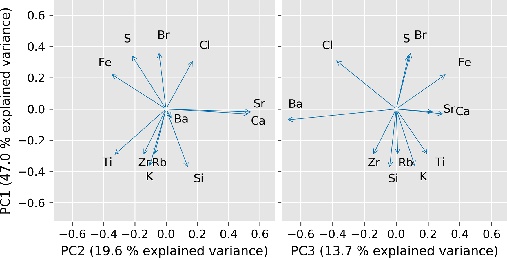
Three reduced dimensions (PCs) in the PCA model, preserving 80.3% of the total variance (Fig. 2), were selected. The scree plot of the explained variance ratio for each PC is provided in Figure S1 (in the supplementary material available online at https://doi.org/10.1017/njg.2021.6). PC1 (47.0% variance explained) shows a negative correlation to the elements Si, K, Ti, Rb and Zr while it is positively correlated to the elements Br, S, Cl and Fe. PC2 (19.6% variance explained) has a conspicuous covariation for Ca and Sr. Fe and Ti have an opposite correlation to Ca and Sr. PC3 has a distinctively negative correlation for Ba.

Fig. 2. PCA loadings from homogenized elemental intensities. The first three principal components together preserve 80.3% of the total variance.
Facies description
There are eight facies (moraine, eolian/fluvial, soil, peat, lagoonal, sand flat, channel fill and beach-foreshore) recognised based on lithology descriptions in the selected sections. The descriptions, according to macroscopic lithological observations accompanied by CT visualisation, are listed below. It should be noted that this observer-dependent facies classification is likely not directly comparable to a classification based on the integration of further (quantitative) measurements, e.g. palaeontological and grain-size data, and provides a rather general facies discrimination. Close-up photographs of the most important facies found in the WASA project are shown by Capperucci et al. (Reference Capperucci, Enters, Bartholomä, Bungenstock and Wehrmann2021).
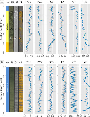
Moraine sediments are characterised by compacted and unsorted sediments (Fig. 3A). Their grain size varies from gravel to silt. Lithic clasts have angular shapes. The sediment has a greyish colour and lacks stratification. The carbonate content is usually low, but whitish carbonate clasts cause a strong reaction with HCl (10%).

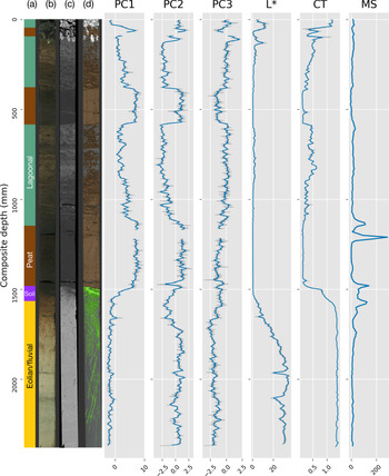
Fig. 3. Cores N14-2 (A) and N33-2 (B): facies labels (a); digital photograph (b); radiograph (c); and sediment constituents (golden: high-density sediments and lithic clasts) separated using CT density (d). Sediment constituents (d) reveal intercalated layer structures and bioturbation. Scores of PC1–PC3 (dimensionless) from elemental intensities, lightness (L*), ranging from 0 (black) to 100 (white), CT density (CT in 103 HU) and magnetic susceptibility (MS in 10-6 SI). Blue lines represent an 8 mm moving average, while grey lines represent raw data. No moving average is applied to MS.
Eolian/fluvial sediments are composed of well-sorted fine sand that lacks sedimentary structures and microfossils. Occasional stratifications and rhizoliths are observed (Fig. 4). The carbonate content is very low. Further differentiation between eolian and fluvial sediments requires further analyses, such as grain-size measurements.

Fig. 4. Core VVC16-3+4: facies labels (a); digital photograph (b); radiograph (c); and sediment constituents (brown: peat; green: rhizoliths; white: shell fragments) separated using CT density (d). Sediment constituents (d) reveal some hidden structures of the core, such as the deeply penetrating rhizoliths. Scores of PC1–PC3 (dimensionless) from elemental intensities, lightness (L*), ranging from 0 (black) to 100 (white), CT density (CT in 103 HU) and magnetic susceptibility (MS in 10-6 SI). Blue lines represent an 8 mm moving average, while grey lines represent raw data. No moving average is applied to MS.
Soils are composed of brown silt to fine sand with a high amount of organic matter, and mark the end of the transition from eolian/fluvial sediments to peat with an unconformity at the top. The high organic matter content starts to decrease rapidly down-core (Fig. 4). Also, multiple rhizoliths are visible in the 3D reconstruction (Fig. 4D) originating from this horizon.
Peat contains dark-brown to black deposits consisting mainly of organic matter. Plant fragments are the dominating components (Fig. 4). Minerogenic components are rarely observed.
Finely bedded greyish silts and intercalated fine sands are observed in lagoonal facies (Fig. 4), containing reworked peat and plant debris, often Phragmites (reed) fragments or rhizomes. The definition of this facies refers to sediments deposited in protected, quiet and shallow brackish environments, possibly behind barrier islands or levees (Streif, Reference Streif2004; Daidu et al., Reference Daidu, Yuan and Min2013). Salt marsh sediments may share similar lithological characteristics, but palaeontological data are lacking so far for better discrimination.
Sand-flat deposits consist of carbonate containing greyish fine sands intercalated by shell fragments and occasional mud layers (Fig. 5A). The macroscopically described grain size varies from fine to medium sand.

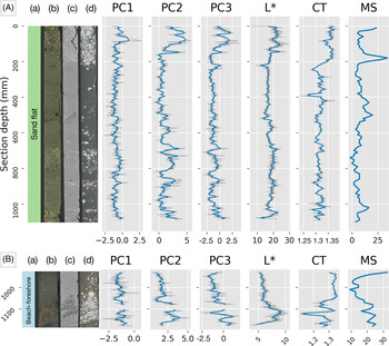
Fig. 5. Cores N35-4 (A) and VVC20-3 (B): facies labels (a), digital photograph (b), radiograph (c) and sediment constituents (white: shell fragments; golden: high-density sediments and lithic clasts) separated using CT density (d). Scores of PC1–PC3 (dimensionless) from elemental intensities, lightness (L*), ranging from 0 (black) to 100 (white), CT density (CT in 103HU), and magnetic susceptibility (MS in 10-6 SI). Blue lines represent an 8 mm moving average, while grey lines represent raw data. No moving average is applied to MS.
Channel fill deposits comprise finely interlayered grey sands and dark grey muds, often showing flaser or lenticular beddings (Fig. 3B). Shell fragments and bioturbation features are rare.
Beach-foreshore deposits consist of fine to coarse sand and layers of brownish shell fragments (Fig. 5B). Their colour ranges from grey to dark grey. Few bedding planes have been recognised.
Collective results of scanning techniques
There are two types of visualisation for scanning measurements of the previously recognised facies. First, the measurements (PC1–3 scores, L*, CT density and MS) are plotted on a depth scale along with facies labels, digital photographs, radiographs and sediment constituents separated by CT density (Figs 3–5). Variations of these measurements denote the spatial distribution of physical and chemical characteristics within and among facies. A steep increase in CT density marks the transition from moraine sediments to channel fill (Fig. 3A), while the intersections of mud and sand in the channel-fill facies itself are denoted by frequent wiggles (Fig. 3B). The PC scores express the changes in peat sections (Fig. 4), while L* and MS show only weak variations. The change from eolian/fluvial sediments to soil is documented by a gradual colour transition (L*), but rather sharp in CT density. Secondly, the measurements’ data distributions are plotted for each facies (density plots: Figs 6 and 7). The PC scores range from −5 to 10, while L* varies from 0 to 40. The values of MS range from 0 to 300 × 10−6 SI. CT-density values vary from 300 to 1700 HU. The shape of the data distributions illustrates the characteristics of each facies. Multiple peaks in a single analyte indicate mixed properties, whereas a single and narrow peak represents a uniform property. Each facies expresses a distinct behaviour based on the shapes and locations of distributions. Detailed characterisations are discussed below.

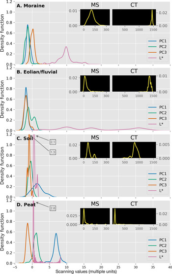
Fig. 6. Density plots of down-core scanning results from terrestrial sediment facies (A: moraine; B: eolian/fluvial; C: soil; D: peat) showing the scores of PC1, PC2, PC3 and lightness (L*). The extreme peak values in density function are noted in text boxes connected with arrows. As inserts, the density plots for magnetic susceptibility (MS) and CT density (CT) are provided. Each curve represents a smoothed and standardized density function of each result. The area below stands for the probability, which sums up to 1. The x-axis is a pure number scale for placing different down-core scanning results on their own unit. For reasons of comparison, the axes are fixed to a certain range. For the raw histograms, which have independent axis ranges, please refer to Figures S4–7 (in the supplementary material available online at https://doi.org/10.1017/njg.2021.6).
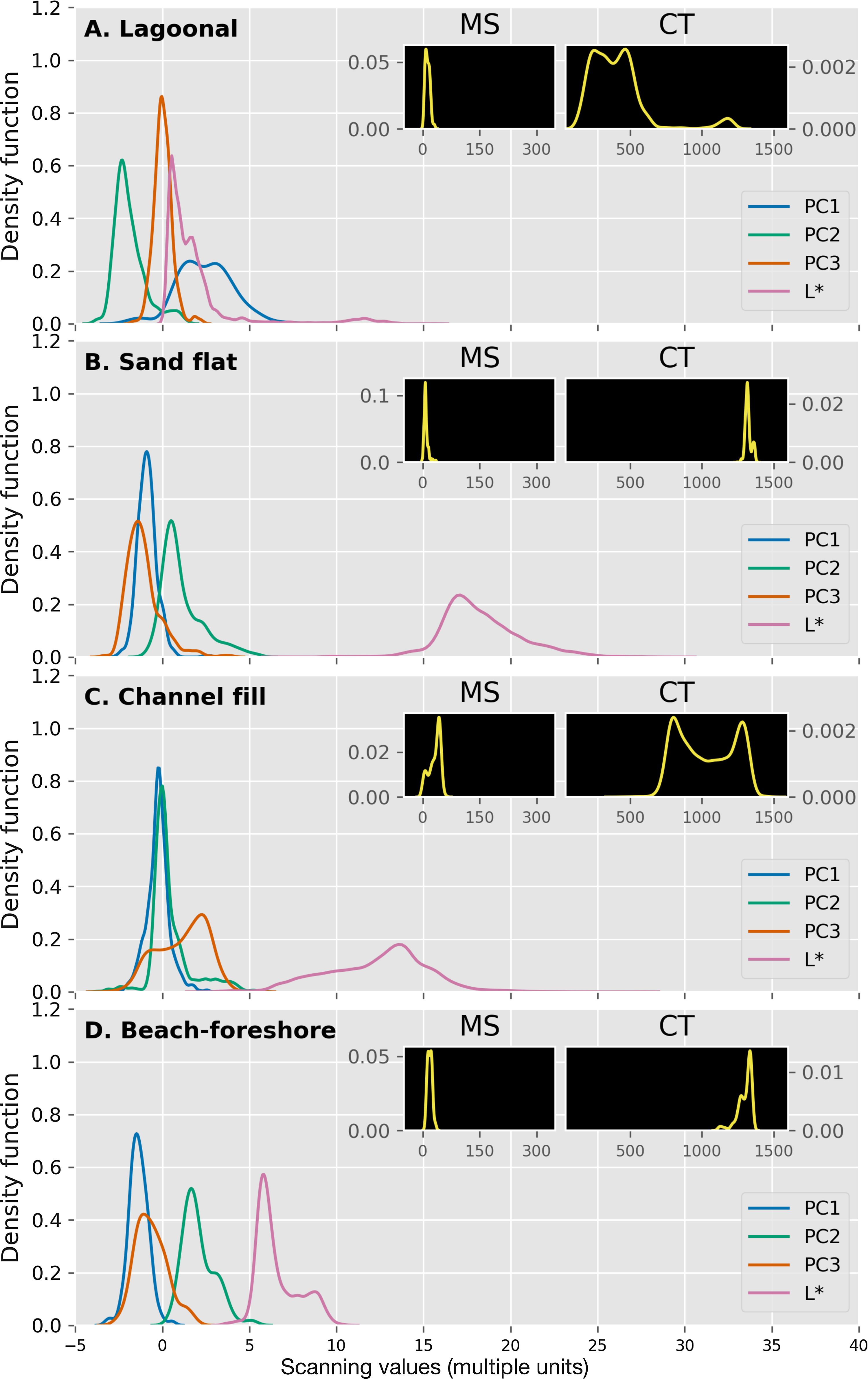
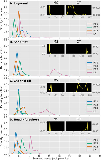
Fig. 7. Density plots of down-core scanning results from marine sediment facies (A: lagoonal; B: sand flat; C: channel fill; D: beach-foreshore) showing the scores of PC1, PC2, PC3 and lightness (L*). As inserts, the density plots for magnetic susceptibility (MS) and CT density (CT) are provided. Each curve represents a smoothed and standardised density function of each result. The area below stands for the probability, which sums up to 1. The x-axis is a pure number scale for placing different down-core scanning results on their own unit. For reasons of comparison, the axes are fixed to a certain range. For the raw histograms, which have independent axis ranges, please refer to Figures S4–7 (in the supplementary material available online at https://doi.org/10.1017/njg.2021.6).
Discussion
Implications of principal component analysis
PC1 shows a negative correlation to the elements related to rock-forming minerals (Si, K, Ti, Rb, Zr) (Fig. 2) (Wang et al., Reference Wang, Zheng, Xie, Fan, Yang, Zhao and Wang2011; Rothwell & Croudace, Reference Rothwell, Croudace, Croudace and Rothwell2015). It also has a positive correlation to Br, S, Cl and Fe, indicating the existence of organic matter and pyrite formation (Sluijs et al., Reference Sluijs, Röhl, Schouten, Brumsack, Sangiorgi, Damsté and Brinkhuis2008). High organic matter content in sediments produces a reducing environment for pyrite to form when accompanied by Fe available from the pore water (Rothwell & Croudace, Reference Rothwell, Croudace, Croudace and Rothwell2015). In addition, the organic matter absorbs Br and Cl due to their high affinity (Keppler & Biester, Reference Keppler and Biester2003; Leri & Myneni, Reference Leri and Myneni2012). This interpretation is supported by the corresponding results of TOC and Br analyses from an accompanying study (Bulian et al., Reference Bulian, Enters, Schlütz, Scheder, Blume, Zolitschka and Bittmann2019). Without conventional grain-size measurements, the usefulness of a common grain-size proxy, e.g. Zr/Rb (Zolitschka et al., Reference Zolitschka, Rolf, Bittmann, Binot, Frechen, Wonik, Froitzheim and Ohlendorf2014), is limited in this study. As a result, PC1 is regarded as an index for distinguishing organic (positive) from lithogenic sediment components (negative). PC2 has a conspicuous covariation for Ca and Sr, which links to biogenic carbonates’ presence (Rothwell et al., Reference Rothwell, Croudace, Croudace and Rothwell2015). In addition, Fe and Ti, presenting in the clay fraction and heavy minerals (Kolditz et al., Reference Kolditz, Dellwig, Barkowski, Badewien, Freund and Brumsack2012a,b), correlate negatively with Ca and Sr. Thus, PC2 is interpreted as enrichment of carbonates, which relates to marine influences (Rothwell & Croudace, Reference Rothwell, Croudace, Croudace and Rothwell2015). PC3 has a distinctively negative correlation for Ba, an element often used as palaeoproductivity proxy (Jaccard et al., Reference Jaccard, Galbraith, Sigman, Haug, Francois, Pedersen, Dulski and Thierstein2009; Ziegler et al., Reference Ziegler, Lourens, Tuenter and Reichart2009) in deep-sea environments. However, this interpretation cannot be transferred to coastal sediments with water depths of <100 m. Besides, it would conflict with PC1 as an expression of organic matter. Thus, the environmental condition causing PC3 (Ba) fluctuations remain unclear. So far, it is essential to note that the PCA depicts only the general covariance between elements of sediment records as a whole. Considering our study’s contrasting depositional environments, a consistent interpretation of a specific element (or PC) across the whole data set may not be feasible.
Facies characterisation
Moraine sediments
The three PCs’ scores distribute in symmetrical and unimodal shapes centred at −1.5 and 0 (Fig. 6A). PC1 and PC2 indicate a lithogenic and terrigenous nature of the sediments. L* supports the greyish colour with a slightly left-skewed distribution centred at a high value of 10. The high values and unimodal shapes of MS and CT density in Figure 6A indicate a high density and more iron-bearing (magnetic) minerals, which corresponds to the interpretation of PC1 and PC2. The lack of bimodal distributions due to the gravel-silt grain-size variance is because: (1) the elemental intensities at gravel sections were mostly excluded due to the low data quality for XRF core scanning, (2) the colours of gravels are not consistent, (3) the CT densities of gravels were excluded, (4) the appearance of gravels is relatively rare (Fig. 3A). We only present one section for this facies in Figure 3A. For the other section containing moraine deposits, please refer to Figure S2A in the supplementary material available online at https://doi.org/10.1017/njg.2021.6.
Eolian/fluvial sediments
The PC1 score (Fig. 6B) is distributed in a unimodal and symmetrical shape and centred at −2, suggesting a lack of organic matter. In contrast to the moraine facies, the PC3 score shifts to negative values and overlaps with PC1. For PC2, scores show a bimodal shape in distribution, located at opposite sides of zero. This may indicate an incomplete carbonate removal or unidentified/unrecognised Eemian marine sediments. Such sediments were found in other cores obtained within the WASA project (Schaumann et al., Reference Schaumann, Capperucci, Bungenstock, McCann, Enters, Wehrmann and Bartholomae2020). The wide range of L* (Fig. 6B), which contains three minor peaks, sets up a unique feature of this facies. Two of the peaks have locations coinciding with the unimodal peaks for moraine (10) and sand-flat facies (17), supporting the multiple sand sources for this facies. The reworking of Saalian till by eolian processes mentioned by Schüttenhelm & Laban (Reference Schüttenhelm and Laban2005) could be one reason. The high CT density and low MS values (close to 0; Fig. 6B) imply a predominantly lithogenic and paramagnetic (i.e. quartz-rich) sediment composition. We only present two sections with this facies (Figs 3 and 4). For the other section, please refer to Figure S2A.
Soil
PC1 and PC2 scores reveal leaching evidence of the soil (Fig. 6C). The increasing PC1 score and the slightly decreasing PC2 score compared to the eolian/fluvial facies imply accumulation of Fe and organic matter, as well as the removal of carbonates due to leaching processes (Reineck & Singh, Reference Reineck and Singh1986). The peak in MS (Fig. 4) at around 1500 mm composite sediment depth indicates the presence of Fe-bearing minerals. The bimodal shape of L* (Fig. 6C) with peaks located at 0.5 and 1.5 supports the darker colours. From the bimodal shape of MS and L* (Fig. 6C), this weathered material has distinct differences in colour and Fe content compared to less weathered sediment. However, due to the small sample size of MS measurements for this facies (Table S2 in the supplementary material available online at https://doi.org/10.1017/njg.2021.6), the MS data are not robust. The relatively symmetrical, unimodal and wide shape of PC1 (Fig. 6C) indicates the balancing mixture of lithogenic sediments, Fe minerals and organic matter. The median value of CT density comparing to the eolian/fluvial and peat facies in Figure 6C, and the variations of L* and CT density in Figure 4 indicate an intermediate stage between eolian/fluvial sediments and peat.
Peat
The lithological descriptions of peat are corroborated by scanning results (Fig. 6D). The unimodal, symmetrical and narrow shape of the PC1 score, located at the highest positive value (7) compared to the other facies types, implies a high organic matter content. The total organic carbon content of up to 38% in peat layers, measured from a neighbouring core, supports this observation (Bulian et al., Reference Bulian, Enters, Schlütz, Scheder, Blume, Zolitschka and Bittmann2019). This agrees with rare lithic components since MS and CT-density values remain close to zero (Fig. 6D). Together with a (probably post-depositional) marine influence, revealed by slightly higher PC2 (c.1.5), an enhanced formation of pyrite, indicated by PC1, seems to describe the coincidence of coastal peat growth, seawater sulphate influence and microbial reduction (Dellwig et al., Reference Dellwig, Watermann, Brumsack, Gerdes and Krumbein2001, Reference Dellwig, Böttcher, Lipinski and Brumsack2002). This phenomenon is supported by the intercalation of this facies with lagoonal sediments (brackish environment). Due to the homogeneously dark colour, values of L* also concentrate close to zero.
Lagoonal sediments
The multiple peaks found in the scanning data (PC1 score, CT density and L*) (Fig. 7A) support the mixture of materials typical for such deposits (Reineck & Singh, Reference Reineck and Singh1986). MS cannot detect this characteristic, probably because its scanning step size is larger than the predominant thickness of the beddings or the difference in Fe-mineral content of this facies is indistinct. If the cause of indistinct Fe-mineral difference can be excluded, it would suggest a predominant bedding thickness smaller than the scanning step size of MS, i.e. 1 cm. The two peaks in the high PC1 score (2 and 4; Fig. 7A) present a mixture of peat debris/organic material and fine-grained minerogenic matter. The three peaks found for CT density may indicate peat debris, lagoonal mud and a few sand grains (from left to right). The bimodal shape of L* backs up these colour changes (Fig. 7A). The unimodal and narrow shape of the PC2 score with a low value of −3 implies an absence of carbonates since they are dissolved by the acidic environment caused by the degradation of organic matter. This corresponds to the CaCO3 undersaturation of the water mentioned by Alve & Murray (Reference Alve and Murray1995). Kolditz et al. (Reference Kolditz, Dellwig, Barkowski, Bahlo, Leipe, Freund and Brumsack2012b) also mention the carbonate-free characteristics of lagoonal sediments for the island of Langeoog. Furthermore, Dijkema et al. (Reference Dijkema, Reineck, Wolff and Group1980) and Streif (Reference Streif2004) describe the existence of lagoons in the transgression cycle (peat – lagoonal clay – tidal flat sands with shells – lagoonal clay – peat) occurring in the Wadden Sea during the early Holocene, which supports the existence of lagoon. Today, this sedimentary environment has largely disappeared, but a few remnants can be found near the islands of Amrum and Trischen and near Sankt Peter-Ording (Ehlers, Reference Ehlers1988). Ehlers (Reference Ehlers1988) describes modern lagoons for the islands of Amrum and Trischen and near Sankt Peter-Ording. Nevertheless, this facies interpretation needs to be confirmed by additional palaeontological data.
Sand-flat deposits
The unimodal and wide shape of L* centred at a high value of 17 (Fig. 7B) reflects the pale colour containing grey sand and whitish shell fragments. The unimodal and narrow shape of both PC1 score and MS, centred at low values (Fig. 7B), indicates the dominance of sand (mostly quartz) in the sediments. The high values of CT density, which are comparable to those of moraine, eolian/fluvial and beach-foreshore facies, support this explanation. The high PC2 score (Fig. 7B) implies the existence of carbonates (i.e. shells). These characteristics (poor in organic matter and rich in carbonates) agree with those found for a tidal sand flat by Bulian et al. (Reference Bulian, Enters, Schlütz, Scheder, Blume, Zolitschka and Bittmann2019). However, this is not supported by distinctly higher CT-density data because the density of shell fragments (>1700 HU) was excluded during CT-density data treatment.
Channel-fill deposits
Since the subtidal channel receives sediments from both sand and mud flats, additionally influenced by tidal movements, these deposits show bimodal characteristics (Fig. 7C) supported by CT density and PC3 score. The unimodal and broad shape of the L* distribution (Fig. 7C) indicates a darker colour compared to the sand flat, and lower colour contrast between mud and sand in the tidal area. Moreover, this low contrast may be induced by averaging data of the lenticular bedding due to the limits of the photograph (2D) while CT density has 3D data points. A slight increase of the PC1 score and decrease of the PC2 score compared to the sand-flat facies imply a subtle signal change caused by the addition of organic matter and dilution of carbonates by the mud-flat sediments. We only present one of the sections with this facies in Figure 3B. The remaining sections are shown in Figures S2–3 (in the supplementary material available online at https://doi.org/10.1017/njg.2021.6).
Beach-foreshore deposits
Brownish shell fragments mark the bimodal distribution of L* (Fig. 7D). The peaks represent dark grey sand and shell fragments (left to right), while the remaining results resemble the sand-flat facies. However, if we look at the three PCs’ relative positions (Fig. 7D), we detect small differences. When taking PC3 as an anchor, the decrease of PC1 and the increase of PC2 scores imply that the deposition is less organic and more carbonaceous (marine), probably due to the lack of protection by the barrier island.
Limits and outlook
Although the combination of scanning results in density plots (Figs 6 and 7) makes comparisons and interpretations convenient, this mixing of data may cause issues due to different applied techniques’ scanning resolution. Scanning resolutions are defined by integration of two parameters, step size and window size. The step size determines the frequency of scanning points. If, for instance, the step size is larger than lamination thickness, the number of lamination is underestimated. In other words, the sampling rate is lower than the signal frequency. This phenomenon bridging the continuous and discrete signals is addressed by the Nyquist–Shannon theorem (Nyquist, Reference Nyquist1928; Shannon, Reference Shannon1949). On the other hand, the window size (e.g. the pixel size of images) determines each scanning point’s scanning window. For example, a data point obtained with a larger scanning window than the thickness of lamination reflects only an averaged lamination value. With different settings of these two parameters, the resolution varies. Francus & Pirard (Reference Francus and Pirard2005) reveal that images taken with the same camera and from the same mineral thin-section but with different resolutions can generate a different phase. This issue occurs in lagoonal sediments of this study. Moreover, the averaging process from 2D and 3D to 1D data creates different levels of boundary blur, which has consequences for the characterisation of finely laminated deposits.
In fact, a sedimentary facies is rarely homogeneous. There are variations of sedimentological and geochemical properties within each facies. For example, a moraine may contain sections of well-sorted sediments (Reineck & Singh, Reference Reineck and Singh1986). Peats can be composed of fen and peat bogs according to nutrient availability (Charman, Reference Charman2009). Soils commonly have different horizons resulting from soil-forming processes (Mack et al., Reference Mack, James and Monger1993). Due to the regional sampling scale of this study and the limited amount of core sections available for analyses, this study cannot include all variations in each facies. Grain size is one of the most important factors to determine sediment facies. This study includes the grain-size discussion based on lithological descriptions and PCA interpretations, but it is not supported by any conventional grain-size measurements. Consequently, facies are simplified to general categories instead of providing a detailed classification, which requires a spatially more diverse sampling database and more quantitative data, such as palaeontological and grain-size analyses. Nevertheless, our approach is the first practical step to analyse the data of different core-scanning techniques to evaluate their potential for facies characterisation.
Machine learning has progressed considerably in various disciplines over the past two decades (Jordan & Mitchell, Reference Jordan and Mitchell2015). Recently, there have been studies developing automatic facies classification on geological records. These deploy a vast variety of variables, including seismic reflection data, petrophysical logging data, hyperspectral imaging or geochemical measurements, to discriminate facies or classify sedimentary structures (e.g. Kuwatani et al., Reference Kuwatani, Nagata, Okada, Watanabe, Ogawa, Komai and Tsuchiya2014; Bolandi et al., Reference Bolandi, Kadkhodaie and Farzi2017; Wrona et al., Reference Wrona, Pan, Gawthorpe and Fossen2018; Ai et al., Reference Ai, Wang and Sun2019; Bolton et al., Reference Bolton, Jensen, Wallace, Praet, Fortin, Kaufman and De Batist2020; Jacq et al., Reference Jacq, William, Alexandre, Didier, Bernard, Perrette, Sabatier, Bruno, Maxime and Arnaud2020). These studies show that the application of machine learning in sedimentology is still at an early stage. Often, input data are limited and applications are restricted to a small study area or few cores since they are experimental studies. Our study contributes to broader facies coverage and data variety (element data, CT-density, L* and MS variations). The density plots combine these scanning data and illustrate the sediment characteristics of each facies visually. The differences among facies confirm the ability to reproduce the sedimentological observations in a digitised perspective. Therefore, there is a high potential to develop automatic facies classification successfully in the near future.
The goal of machine learning is to train computers to use exemplary data to solve a given problem (Alpaydin, Reference Alpaydin2014). Based on sedimentological expertise, machine learning builds a facies discrimination model in the digital world. The scheme of developing an automatic facies classification using digitised information will be applied on a local scale with general facies classification first, and subsequently progresses to a larger scale and finer classification to cover a higher facies variability. With extended data coverage, inconsistencies and conflicts between results of different studies may appear. For instance, different facies recognitions are made based on different approaches. Nevertheless, we anticipate that future facies classification will be less time-consuming and allow sedimentologists to focus on other critical scientific questions.
Conclusions
This study demonstrates that eight ‘a priori’ recognised sediment facies (moraine, eolian/fluvial, soil, peat, lagoonal, sand flat, channel fill and beach-foreshore) are (semi-)quantitatively characterised and differentiated by their physical and chemical properties obtained by scanning techniques (MS, CT, µ-XRF, digital photography). The application of density plots offers a comprehensive way of presenting these properties and reveals distinct differences between facies. We document that conventional lithological descriptions can be reproduced by time- and cost-efficient (semi-)quantitative and high-resolution digital measurements. However, some facies (lagoonal/salt-marsh sediments and eolian/fluvial deposits) remain arguable, as scanning data show differences that were not previously recognised by conventional facies analysis. After all, digital scanning data are useful for further studies. Based on these results, an automatic facies classification model will be developed by applying machine learning techniques. In the end, a wealth of sedimentary information will be released from the shackles of the expensive and observer-dependent data of the past.
Acknowledgements
The present study is part of the Wadden Sea Archive (WASA) project funded by the ‘Niedersächsisches Vorab’ of the Volkswagen-Foundation within the funding initiative ‘Küsten und Meeresforschung in Niedersachsen’ of the Ministry for Science and Culture of Lower Saxony, Germany (project VW ZN3197), coordinated by the Lower Saxony Institute for Historical Coastal Research (NIHK). We appreciate the WASA project team that jointly carried out the core recovery and macroscopic sediment description. A.S.L. thanks the National Taiwan University (NTU) Research Center for Future Earth from the Featured Areas Research Center Program within the framework of the Higher Education Sprout Project funded by the Ministry of Education of Taiwan for travel support. J.T. received funds from the MARUM Cluster of Excellence ‘The Ocean Floor – Earth’s Uncharted Interface’ (Germany’s Excellence Strategy – EXC-2077 – 390741603 of the Deutsche Forschungsgemeinschaft DFG). We thank the Klinikum Bremen-Mitte and Prof. Dr Arne-Jörn Lemke and Christian Timann for providing their facilities and supporting the performed computed tomography measurements.
Supplementary material
To view supplementary material for this article, please visit https://doi.org/10.1017/njg.2021.6


 Open access