

1. INTRODUCTION
How can we notate timbre as a musical parameter? The background for this work is my research in notation for acoustic and electroacoustic music. In order to sufficiently describe musical structures today, one must sooner or later deal with the concept of timbre.
Van Elferen talks of the exactness of sonorous qualities demanded by composers and how timbres are at the same time idiosyncratic and unrepeatable (van Elferen Reference van Elferen2017). Indeed, describing timbre as a musical parameter is complicated by the fact that there is no consensus on what it really is. However, clarifying the purpose of one’s inquiries makes it easier to find common ground. And therein lies one key to the mystery of timbre: depending on what you want to do with it, you may need a different approach.
A classic definition is that timbre is what differs when two different instruments play the same note with the same dynamics (ANSI 1973). It would therefore be associated with the act of recognising instruments. But then there is the question of constancy since, as Risset and Wessel point out, we recognise a saxophone also when heard over a pocket-sized radio (Risset and Wessel Reference Risset, Wessel and Deutch1999). Also, an instrument’s timbre is not necessarily consistent over its playable range. And many have questioned the idea of timbre as independent of pitch (Smalley Reference Smalley1994; McAdams and Giordano Reference McAdams, Giordano, Hallam, Cross and Thaut2009). In fact, it seems to rely on most if not all other musical parameters. Still, the ANSI definition is reflected in research into the recognition of musical instruments. Furthermore, Pierre Schaeffer acknowledges this definition in his treatise but notes that it ‘far too pragmatic, is crying out to be superseded’ (Schaeffer Reference Schaeffer2017: 45).
Denis Smalley suggests that timbre is ‘a general, sonic physiognomy whose spectromorphological ensemble permits the attribution of an identity’ (Smalley Reference Smalley1994: 38). Stephen McAdams and Meghan Goodchild provide a similar definition: ‘We define timbre as a set of auditory attributes—in addition to those of pitch, loudness, duration, and spatial position—that both carry musical qualities, and collectively contribute to sound source recognition and identification’ (McAdams and Goodchild Reference McAdams, Goodchild, Ashley and Timmers2017: 129). Both confirm the dual nature of timbre that can be related to the difference between describing (changing) aspects as opposed to (recognisable) instances of timbre. In timbre recognition, be it in technology or by human ears, a pre-defined or learnt instance of timbre is either recognised or not. When describing aspects of timbre, one is more interested in what qualities or parameters differ between two instances. Since both these approaches are used in music listening (we identify a sound but we also experience how it changes over time), a musically relevant description of timbre would need to accommodate both these perspectives.
It is apparent that the concept of timbre has different meanings depending on the focus and field of the research. It is true that the ANSI definition is not accepted as a complete explanation of the phenomenon. At the same time, it is a practical way of dealing with timbre in the comparison of equivalent instances of different musical instruments. Also, a more comprehensive definition, even if considered closer to the true nature of timbre, risks embracing too many parameters to have any practical value. It also seems that one source of confusion regarding this phenomenon is how it seems to correspond to what in Swedish and German are two different concepts: (in German) klang and klangfarben. Simply put, the former is a more general term for a sound’s characteristics while the latter is more oriented towards the spectral aspects of a sound. The broader definition of timbre also includes all qualities of a sound’s energy contour. In other words, timbre relies both on colour and form. This relates to Schaeffer’s concepts of mass and facture (Schaeffer Reference Schaeffer2017), which in Thoresen and Hedman were adapted to sound spectrum and energy articulation (Thoresen and Hedman Reference Thoresen and Hedman2007). So the ANSI definition works with the notion of timbre as sound spectrum while Smalley’s more elaborate definition also includes the spectrum’s morphology.
Before introducing my notation solutions for the spectral aspects of timbre as a (multidimensional) musical parameter, I will provide some context within the growing field of timbre research, beginning with auditory stream segregation, dealing with the question of what constitutes one instance of timbre. Schaeffer made the sound object his starting point for his classification and description of a sound event (Schaeffer Reference Schaeffer2017). I will hereafter use this term to represent the delimited audio material that one decides to notate as one notation object. I use the term regardless of Schaeffer’s idea of reduced listening – a listening without considering sound source(s).
2. OVERVIEW OF TIMBRE RESEARCH
2.1. Auditory stream segregation
Bregman introduced auditory scene analysis (Bregman Reference Bregman1990) as a way of dealing with the problem of auditory stream segregation, it is ‘the process whereby all the auditory evidence that comes, over time, from a single environmental source is put together as a perceptual unit’ (Bregman Reference Bregman, McAdams and Bigand1993: 11). This can happen either in relation to sets of sound characteristics familiar to us, or as a result of more ‘primitive’ methods where the acoustic properties of the sounds themselves suggest they belong to one and the same sound source. Even if we advocate a listening removed from recognition of sources, we rely on auditory scene analysis to explain how we differentiate between the layers of a sound structure.
It is worth noting that what is perceived as a single sound object (and possibly a single source) can consist of several different spectral components heard both separately and as parts of a shared sound object. This can, for example, occur with percussion instruments where the impact of a mallet on an instrument body will produce a sound in both the mallet and the instrument. In such cases removing the attack will radically change the perception of the sound object.
2.2. Timbre perception and description
In his seminal work on timbre perception, John M. Grey explored timbre differences of acoustic instruments in listener tests where differences were displayed using multidimensional scaling (MDS). This resulted in instrument timbres positioned in a 3D model whose three axes were interpreted as relating to spectral energy distribution, synchronicity of higher harmonics of the transient, and the presence of low-amplitude, high-frequency energy (Grey Reference Grey1977). They explored these characteristics further by introducing spectral modifications to the sound pairs (Grey and Gordon Reference Grey and Gordon1978). The confirmed acoustic dimensions defining this geometric space, later referred to as the timbral space (Wessel Reference Wessel1979), are: spectral centroid, attack time and spectral irregularity (McAdams and Giordano Reference McAdams, Giordano, Hallam, Cross and Thaut2009). The spectral centroid relates to the perceived spectral brightness, the attack time relates to sound onset characteristics, and spectral irregularity relates to the consistency and stability of a spectrum over time. These are divided between the frequency domain (spectral centroid and irregularity) and the time domain (attack time).
Grill and colleagues approached the description of sound texture timbre with a mixed qualitative-quantitative perspective. Listeners were asked to describe timbre differences in their own words in a process that resulted in five constructs with over 50 per cent agreement among expert listeners: high-low, ordered-chaotic, smooth-coarse, tonal-noisy and homogeneous-heterogenous (Grill, Flexer and Cunningham Reference Grill, Flexer and Cunningham2011). Štěpánek, like Grill, performed a study with verbal attributes but with musical instruments. He concludes, among other things, that the saliency and relationship between the verbal constructs and the real sounds were sound context dependent (Štěpánek Reference Štěpánek2006). So when describing timbre in notation we may need to ask ourselves whether a sound spectrum is perceived as bright in absolute or relative terms. Lemaitre and colleagues explored the use of verbal sounds and hand gestures to describe timbre. They found a general consistency in terms of what timbral features that were represented verbally and through gestures as well as agreement regarding the type of gestures used for describing a particular sound. The multi-dimensionality of timbre was exemplified by one of their participants describing different timbre aspects with his voice and his hands in reaction to a sound with both tonal and noisy components (Lemaitre, Scurto, Francoise, Bevilacqua, Houix and Susini Reference Lemaitre, Scurto, Francoise, Bevilacqua, Houix and Susini2017).
De Poli and Prandoni speak of two important variables involved in timbre research: 1) the instruments used for analysis and modelling of the timbre, and 2) the techniques used for representing the data, referring to this as a sonological model (De Poli and Prandoni Reference De Poli and Prandoni1997). Aural sonology is also a description of Lasse Thoresen’s research on music analysis. His spectromorphological analysis builds on ideas and concepts from Pierre Schaeffer (Reference Schaeffer, North and Dack2012) and Denis Smalley (Reference Smalley1997) providing a versatile symbolic system for describing music as heard (Thoresen and Hedman Reference Thoresen and Hedman2007). Also, Schaeffer’s Treatise on Musical Objects (Schaeffer Reference Schaeffer2017) can be read as a theory of timbre perception, going far beyond his concise typology of sound object categories.
2.3. Timbre classification through sound synthesis
For timbre research on musical instruments, synthesised versions of the instruments were often used; for example, FM synthesis (Krumhansl Reference Krumhansl1989; Krimphoff, McAdams and Winsberg Reference Krimphoff, McAdams and Winsberg1994; De Poli and Prandoni Reference De Poli and Prandoni1997). FM synthesis has been used to explore timbre associations (Wallmark, Frank and Ngheim Reference Wallmark, Frank and Nghiem2019). Ashley also uses FM synthesis but with the roles reversed; instead of using FM synthesis to explore timbre description, timbre description is used to control timbre-oriented sound design with FM synthesis (Ashley Reference Ashley1986). Similarly, Grill relies on descriptions and visualisations of timbre derived from audiovisual correspondences to aid in the browsing of large sets of texture sound files (Grill and Flexer Reference Grill and Flexer2012).
Research connecting timbre characteristics with sound synthesis can be an asset in the development of timbre notation, since sound synthesis is governed by limited sets of parameters. If we can find a link between timbral features and sound production, this link can possibly be exploited for notational purposes. Here FM synthesis is of interest since it can produce a rich variety of timbres using very few parameters (Chowning Reference Chowning1977). A disadvantage of this approach is how FM-synthesis parameters are unrelated to sound perception. In that regard, physics-based sound synthesis may be more suitable. It can also produce diverse timbres from few parameters, but is rooted in the real world of sounding objects, making its parameters more intuitive than FM synthesis parameters. Projects such as the Sound Design Toolkit make it possible to implement physics-based synthesis in interactive sound design, making the exploration of timbre both accessible and flexible (Monache, Polotti and Rocchesso Reference Monache, Polotti and Rocchesso2010).
Regardless of the use of sound synthesis for timbre description, this research will be of importance once the notated structures are subject to software playback.
2.4. Source recognition
Timbre is important for source recognition. In 1964 Berger explored this by having listeners identify woodwind and brass instruments even when played backwards, through steep low-pass filters or with the first and last half second cut out (Berger Reference Berger1964). He found it was particularly difficult for listeners to identify the low pass filtered sounds (18 per cent), as well as the sounds with attack and decay removed (35 per cent). However, results were much improved if he accepted correct classification into the overarching instrument families (woodwind or brass). That listeners, even for modified recordings, could recognise instruments based on their material and sound production suggests that a timbre description model related to the recognition of timbre categories, such as wooden or metal sounds, can be a way forward.
There is also research on computers’ capacity to recognise sounds. Agostini and colleagues found that the most relevant timbral features for source recognition were inharmonicity, spectral centroid and energy of the first partial (Agostini, Longari and Pollastri Reference Agostini, Longari and Pollastri2003).
Historically source recognition has been a dividing issue in electroacoustic music because of narrative listening being frowned upon in art music (Emmerson Reference Emmerson and Emmerson1986), prompting the pioneers of electroacoustic music to advocate a reduced listening with no regard to sound sources (Schaeffer Reference Schaeffer2017). However, sound sources are integral to the music theory of both acoustic and electroacoustic music, particularly with regard to timbre. But source and timbre are not the same – one sound source can produce different timbres.
2.5. The audiovisual crossmodal correspondence of timbre
When defining symbolic notation of timbre as a musical parameter, it makes sense to also consider correspondences between sound and image in this regard. In his extensive review, Spence defines crossmodal correspondence as ‘a compatibility effect between attributes or dimensions of a stimulus (i.e., an object or event) in different sensory modalities (be they redundant or not)’ (Spence Reference Spence2011: 973). The correspondences occur so that an extreme value in one modality should correspond to an extreme value in the other modality. A classic example is how the ‘i’ and ‘a’ vowels were found to be associated with small and large objects respectively (Sapir Reference Sapir1929). Later studies have establish audiovisual crossmodal correspondence (AVC) between auditory pitch and the visual modalities: elevation, brightness, lightness, shape/angularity, size, spatial frequency and direction of movement. Also auditory loudness has been found to correspond to visual brightness (Spence Reference Spence2011).
Adeli and colleagues studied specifically the AVCs between musical timbre and visual shapes. They found that a harsh timbre related to a sharp jagged shape while a soft timbre related to a rounded shape. Interestingly, a timbre with a mixture of soft and harsh timbral elements, such as the saxophone, equally corresponded to a mixed shape of sharp and rounded angles (Adeli, Rouat and Molotchnikoff Reference Adeli, Rouat and Molotchnikoff2014). Also, their study showed that shape selection for certain harmonic sounds (cello and guitar) depended on fundamental frequency, with rounded shapes for lower fundamentals and partly angular shapes for higher fundamentals.
There has been implementations of timbre-related AVC in the user interfaces of music software. One example is Sound Mosaics (Giannakis Reference Giannakis2001, Reference Giannakis2006), starting from Ware’s reasoning that visualisations can be sensory or arbitrary (Ware Reference Ware2000). Inspired by Giannakis, Grill and colleagues developed a user interface for navigating a sound texture library building on their previous research on perceptual qualities of textural sounds (Grill, Flexer and Cunningham Reference Grill, Flexer and Cunningham2011). Their auditory-visual relations are:
-
High→low – brightness+colour hue
-
Ordered→chaotic – texture regularity (position)
-
Smooth→coarse – jaggedness of element outline
-
Tonal→noisy – saturation
-
Homogeneous→heterogeneous – colour variability.
Their tests showed a 46.6 per cent mean hit rate for expert listeners in examples of choosing between five images for a given sound (above the 20 per cent baseline for random selections). Listening conditions and expertise had a significant impact on the results. The associations that were most often confused were the constructs tonal–noisy/smooth–coarse and the constructs homogeneous–heterogeneous/ordered–chaotic (Grill et al. Reference Grill, Flexer and Cunningham2011).
It is wise to address AVC when connecting sound and image for others to interpret, since by not taking AVC research into account, you risk producing a system that is counter-intuitive (Giannakis Reference Giannakis2006). The most important AVC considered for my notation is the connection between pitch and frequency in the audio domain and height in the visual domain.
3. THE NOTATION OF SPECTRAL ASPECTS OF TIMBRE
A notation that is usable for both analysis and composition should reflect both the perception of timbre and its acoustic properties. Considering the preceding timbre definitions, it should also be capable of reflecting timbre’s role in source recognition. Musical qualities and source identity should be indicated in ways that make sense for both perceptive and descriptive purposes. Because of the multiple parameters involved in the appreciation of timbre, we cannot necessarily imagine the interpolation between two timbre instances. What we can do is imagine one particular timbre instance and then envision specific changes to it. As an example, by recalling the culturally shared timbre identity of a piano tone of a certain frequency, amplitude and duration, and then considering this timbre with decreased brightness, we have used a combination of timbre identity and acoustic properties to describe timbre characteristics with far better precision than if we only consider combinations of acoustic properties.
With a notation based solely on acoustic properties related to timbre, there is a risk of conveying little if anything of the experience of timbre. But as stated earlier, there are correlations between the established acoustic properties of timbre space and music parameters used for the analysis of electroacoustic music. So going back to Thoresen’s phenomenological approach to describing music, we can look for correlations between the qualities of sound he describes and how they possibly rely on, and relate to, acoustic properties of sound. So my approach to notating timbre is to adapt Thoresen and Hedman’s notation symbols to describe acoustic qualities relevant for the perception of timbre. For the sake of limiting the scope of this text, the notation presented in the following sections is focused on the spectral aspects of timbre.
3.1. Identification and classification of sound objects
When addressing the identification and classification of individual sound objects, the notation’s purpose is crucial. For traditional music, a transcription is often a form of reverse-engineering of the music, related to the possibilities of known musical instruments. In spectromorphological analysis, focus is on what is heard as separate sound objects regardless of their actual origin. Both approaches are relevant for composition and analysis and they are not polar opposites; the latter approach can be thought of as a prerequisite for the former. Before deducing what actions were performed by a musician, one must consider the music as heard.
At this stage, the spectrum categories must be defined. This is important because it affects how changes in acoustic properties are perceived. I use the three spectrum categories and symbols from Thoresen’s analysis displayed in Figure 1. Thoresen took Schaeffer’s category N (definite pitch) and X (complex pitch, i.e. without pitch) (Schaeffer Reference Schaeffer2017) and introduced the dystonic category representing inharmonic spectra and cluster sounds (Thoresen and Hedman Reference Thoresen and Hedman2007). This categorisation complies with auditory scene analysis principles of spectral integration (with regard to the pitched category) and also with the dimension of spectral irregularity in the timbre space. The circle-shaped pitched category symbols are placed at the position of the root frequency of the spectrum and the diamond-shaped dystonic category symbols are placed at the position of the most notable pitch component of the spectrum. The square-shaped complex category symbols are placed at the position of the spectral centroid, which is the centre frequency of the sound’s spectral energy. This is because in the absence of notable pitch components, the spectral centroid is what I found to be the best indicator of how complex sound objects relate to one another.
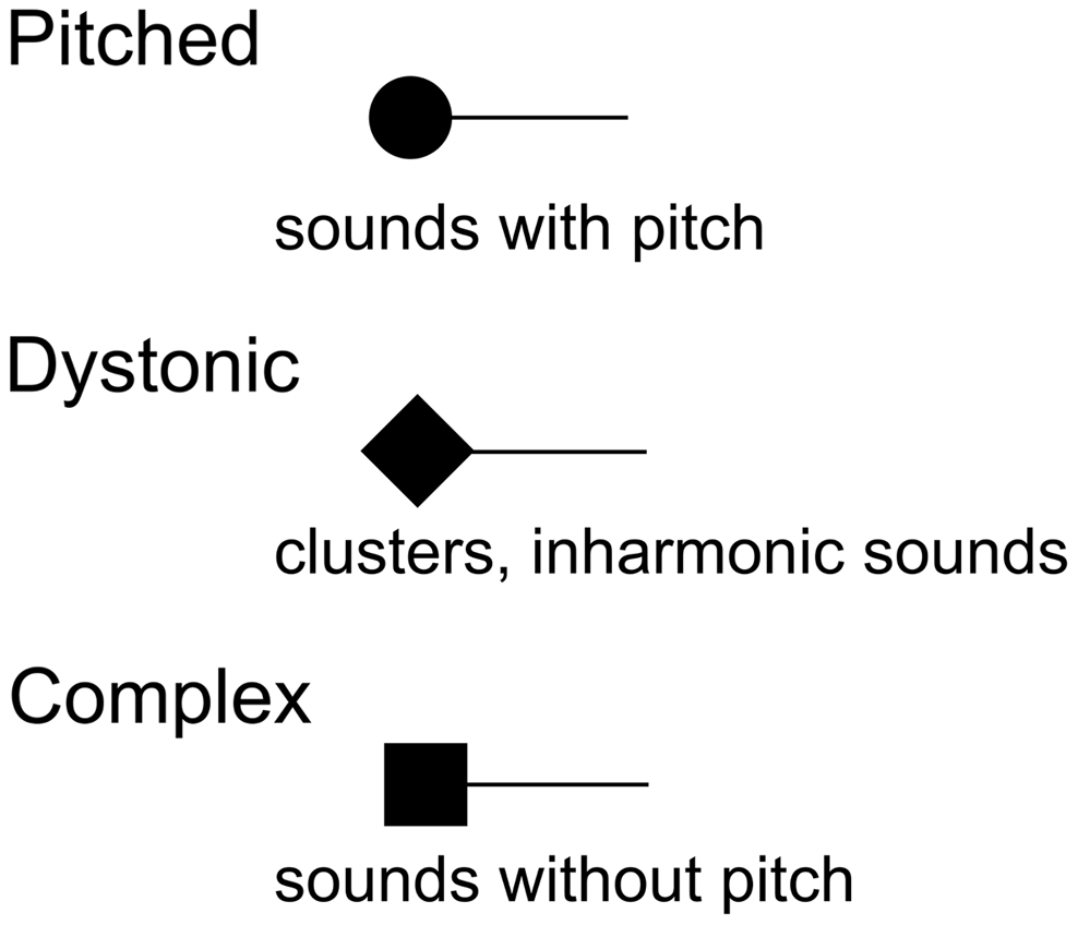
Figure 1. The three spectrum categories and their symbols from Thoresen’s spectromorphological analysis (Thoresen and Hedman Reference Thoresen and Hedman2007).
Often a simple spectrum classification is not enough. A sound object can be a combination of any number of the same or different spectrum categories. What combinations of spectra that would be perceived as one and the same sound object relies on a variety of factors, such as spatial position, perceived size and the same time of onset.
3.2. Spectral width
Not part of Thoresen’s analysis, spectral width is the frequency range of a sound’s spectrum with the highest energy, that is, the loudest partials. It relates in part to the vertical axis of Grey’s timbre space, representing spectral bandwidth or energy distribution (Grey Reference Grey1977). This is defined here as the frequency range of a sound within the amplitude range of -12 dB to 0 dB where 0 dB is the peak amplitude. This provides valuable information for both the mixing and the orchestrating composer (see Figure 2). The -12 dB threshold was selected for pragmatic reasons, based on the author’s experience with audio mixing. Sounds will likely have spectral energy also below -12 dB, but indicating the full frequency range of a sound is not practical for music notation purposes since it would demand additional indications of the magnitude of spectral energy to be useful.
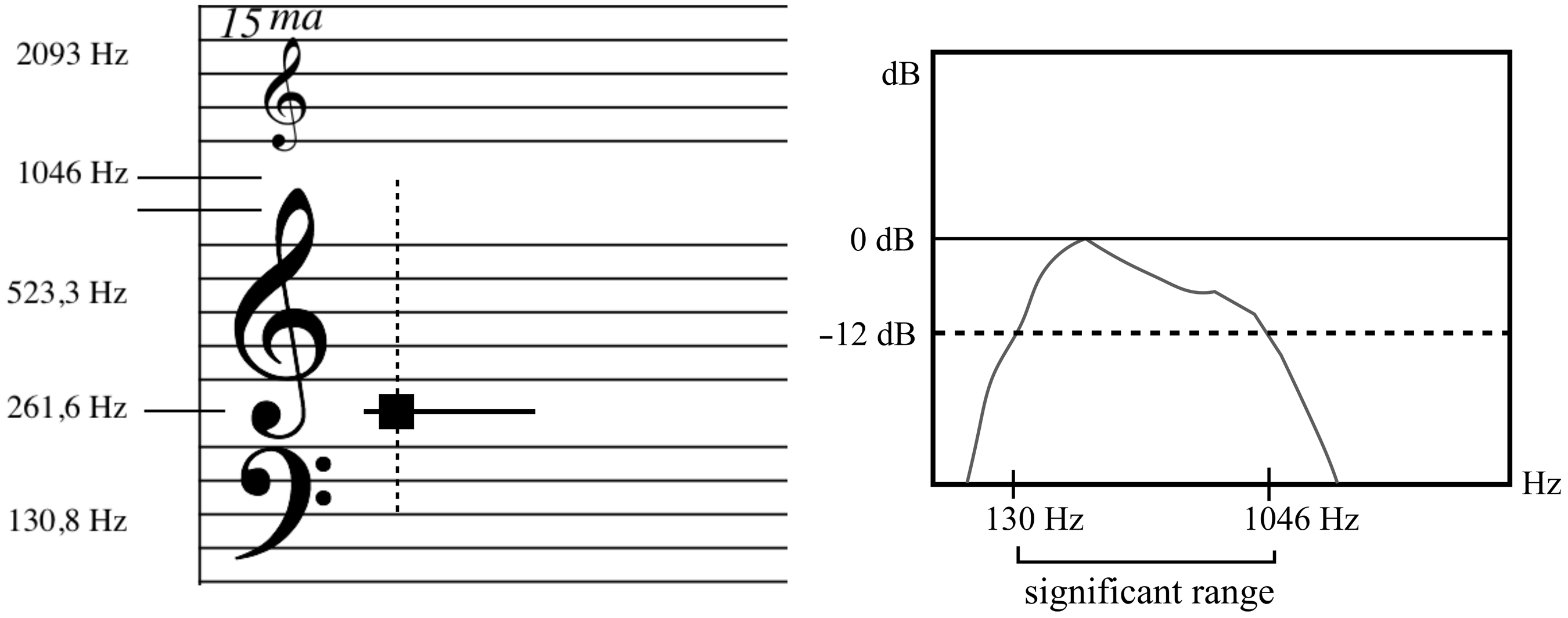
Figure 2. In the notation example, the dashed vertical line indicates spectral width, the frequency range of a sound’s spectrum with the highest energy. The spectrum view to the right shows how one can determine this range for a sound with the peak amplitude of 0 dB, noting the frequency range between 0 dB and -12 dB.
Changes in spectral width are perceived differently depending on spectrum category. Decreasing the spectral width of a pitched sound as shown in Figure 3 (example A) – for example, by using a low pass filter – will result in an audible difference but the root (and therefore the notated position of the note) will remain the same. In example B, the notated position of the note changes with the spectral width since complex sounds are notated at the position of the spectral centroid.
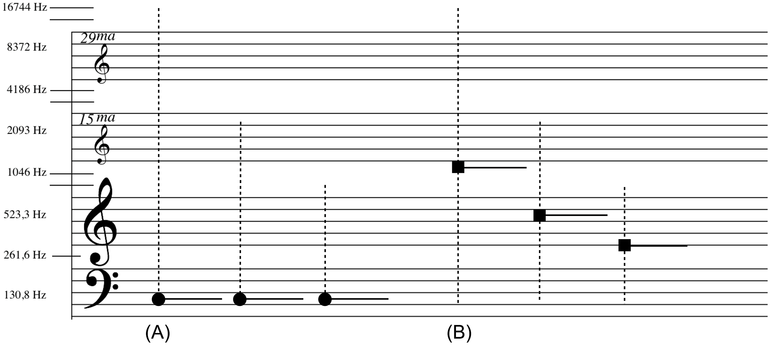
Figure 3. Comparison of lowering the upper limit of spectral width for three occurrences of a pitched sound (A) and a complex sounds (B) and how the notated position changes for the complex sound but not the pitched sound.
There are also differences to consider related to acoustic and electroacoustic sound sources. Using sound synthesis, one can produce extreme examples of spectral width not possible with acoustic instruments from the sine wave (theoretically) without partials to the sawtooth wave with high amplitude partials for the whole spectrum. Another important difference is how one can use filters to produce spectra with little or no frequency content for specific frequency bands.
3.3. Spectral centroid and density
The spectral centroid is the frequency indicating the centre of mass of the spectrum of a sound. It is an important factor for the perceived brightness of a sound, though other factors such as frequency range also play a part. It is also an important feature for timbre classification (Agostini et al. Reference Agostini, Longari and Pollastri2003). In my notation system, spectral density is a relative measurement of the density of a spectrum as a result of the extent to which partials with high amplitude are found close together in the spectrum. To indicate spectral density, I use a comb-like symbol where different numbers of teeth indicate degree of density. This is in line with Thoresen and Hedman’s symbol for spectral saturation that I understand to mean the same thing though it is positioned differently and is not concerned with measurable acoustic properties (Thoresen and Hedman Reference Thoresen and Hedman2007). I place the density symbol at the position of the spectral centroid, unless it is a complex sound, for which it is placed above the symbol. The number of comb teeth vary from two (high density) to six (low density). There is one type of spectral density I think needs a different density symbol and that is the harmonic spectra with only every other partial. This is commonly considered to result in the experience of a ‘hollow’ timbre. This is, for example, the case with the clarinet and the triangle wave on synthesisers. I use a specific comb symbol for such occurrences with every other tooth shortened. There is also a special case where the symbol is completely solid, to indicate maximum spectral density, used for noise.
Figure 4 provides an example of a dystonic sound with a dense spectrum (A) and a pitched sound with only every other partial present and less density (B). Spectrograms of the two sounds (FM-bell and clarinet) are also shown for comparison.
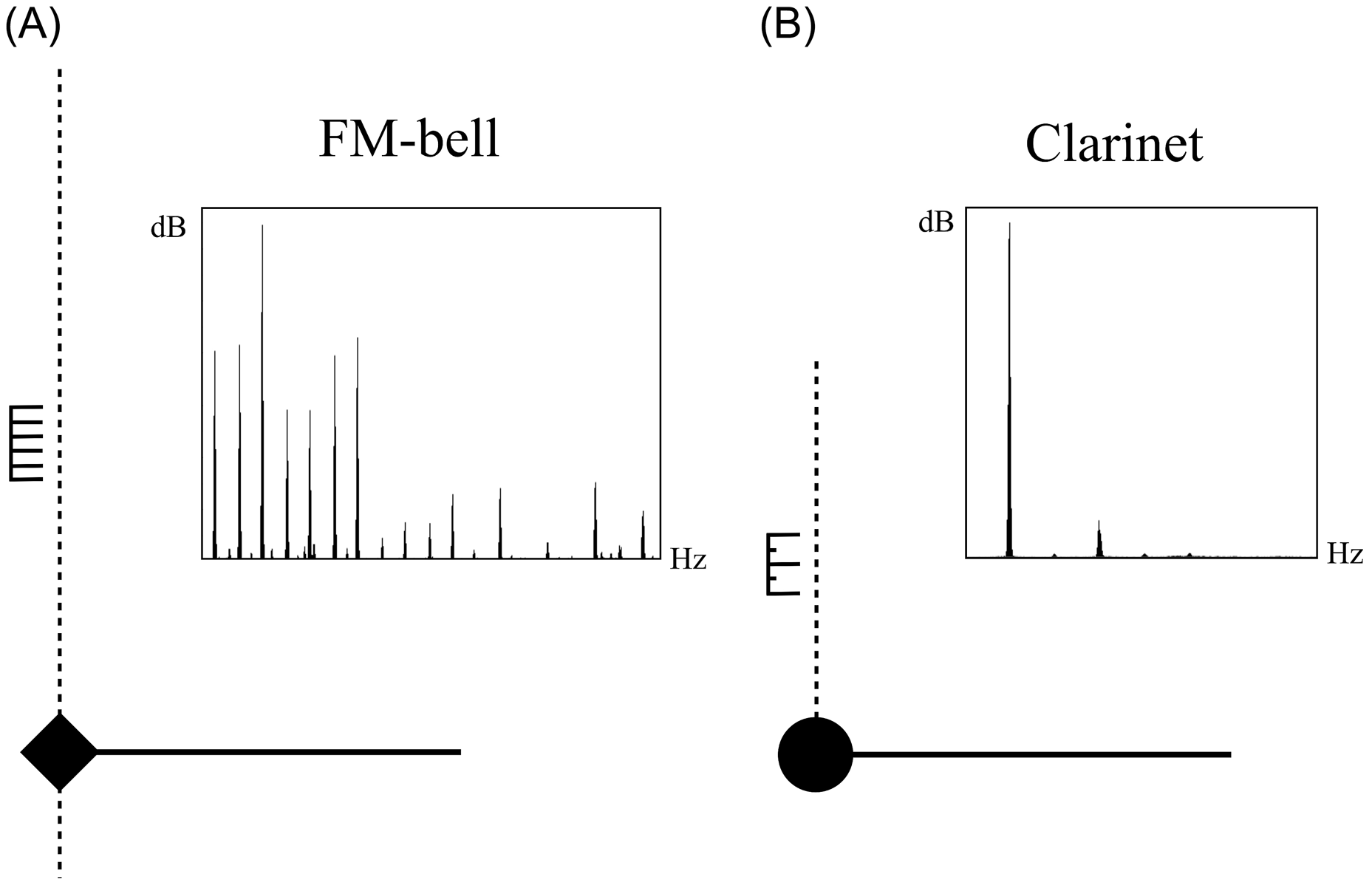
Figure 4. Two sounds with indicators for spectral density (the comb-like symbol by the vertical spectral width line) at the position of the spectral centroid of the sound. For comparison, spectra for the two sounds are also displayed. Example A is of a dense bell-like sound while B is a clarinet, calling for the density indicator to indicate that only every other partial is present.
3.4. Chords and spectral components
A sound object can consist of a combination of spectra. These are notated as chords when they appear to have equal importance, meaning note heads of equal size. Spectral components can appear as aspects of another spectrum and are notated with small note heads. Any spectrum category can be a component of another. A pitched sound may have a noise component that defines its spectral qualities; for example when a woodwind instrument performer lets out an audible noisy stream of air while playing. Pitched components are often needed when transcribing sounds with inharmonic spectra (belonging to the dystonic category), such as church bells. These can have clearly audible pitch components not related to a shared root frequency. Figure 5 shows a dystonic sound where 330 Hz (E4) is considered the main partial of the spectrum and therefore marks the position of the symbol, while 740 Hz (F♯5) is considered a notable pitch component.
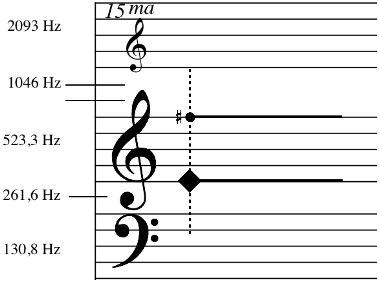
Figure 5. A dystonic sound with a significant partial (740 Hz/F♯5) indicated with a small note head over the spectral width line.
3.5. Spectrum reference
As previously stated, a key feature of timbre is its function for identification and recognition of a sound. This function can be used to describe very particular instances of timbre. If I introduce a shared spectrum reference, such as the clarinet, to the notation of a sound object, the sound’s spectrum is described at a level of detail that would be hard to achieve only using symbolic notation of spectral features. Spectrum reference is indicated in two ways, either as the similarity of a referenced spectrum or as something being that referenced spectrum (see Figure 6). Regardless of the occurrence of shared references, adding spectrum references to the notation of sound objects can be useful for indicating recognisable similarities between sounds of a musical structure.
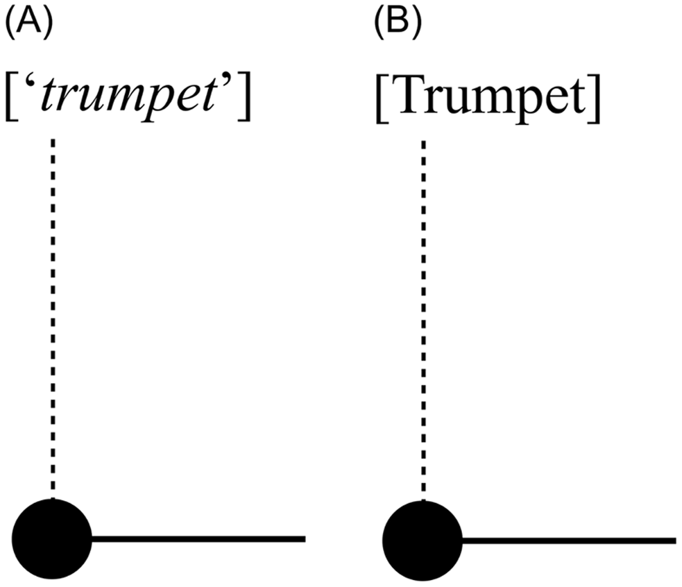
Figure 6. Timbre reference indicated in terms of sounds like a trumpet (A) and is a trumpet (B)
3.6. Time and space
When dealing with timbre as the full experience of a sound, energy articulation is of great importance. Thoresen and Hedman have in their adaptation of Schaeffer’s typomorphology a well-defined system for describing sound structures also in terms of their articulation over time. Another aspect of sound is how it occupies space. Though I have limited the focus of this text to the notation of spectral features of sound objects, I will briefly mention the concepts I use for the notation of time and space. Variation is introduced in the form of modulation as a multipurpose way of handling continuous or discontinuous changes to any parameter. This relates to Schaeffer’s allure that Thoresen and Hedman adapted; for example, in their notation symbols for pitch gait. I use specific indicators for a sound’s amplitude envelope below the notated sound object while the overall dynamics for a staff system can use either classic dynamic markings or the kind of volume automation curve familiar to audio software users. Rhythm itself is represented as a combination of traditional music notation on separate staves and the relative lengths of extension lines from the sound objects’ note heads. This was covered in greater detail in an earlier paper (Sköld Reference Sköld2019a). Notating spatial positions is of particular interest for electroacoustic music, and the symbols I use for displaying positions and movements are similar to the graphical user interfaces used for 2D and 3D panning in audio software. This and additional symbols for spatial sound were also covered in an earlier paper (Sköld Reference Sköld2019b).
3.7. Parameter changes
An important aspect is how the notation can accommodate parameter changes. As in the Thoresen and Hedman analysis notation, all notated parameters presented here can change over time. Visually this works differently for different parameters. Parameters with discrete symbols, such as those for spectral density, change by producing a new symbol along the timeline. Other parameters, such as the higher limit of spectral width change with a dashed line tracing the value changes over the spectrum staff. The ability for parameters to change is also reflected in the MIDI-like data format that accompanies the notation for use with algorithmic composition.
4. EVALUATION: TRANSCRIPTIONS OF ELECTROACOUSTIC MUSIC
To demonstrate the notation system’s ability to describe timbral structures, three short excerpts from classic electroacoustic music works are presented as sound notation transcriptions (scores created from music as heard). These were made by the author using only the audio files, not consulting scores or analyses of the works. In order to indicate the spectral parameters properly, a digital audio workstation was used for playback and real-time spectrum analysis. The transcriptions are shown in Figures 7 to 9.
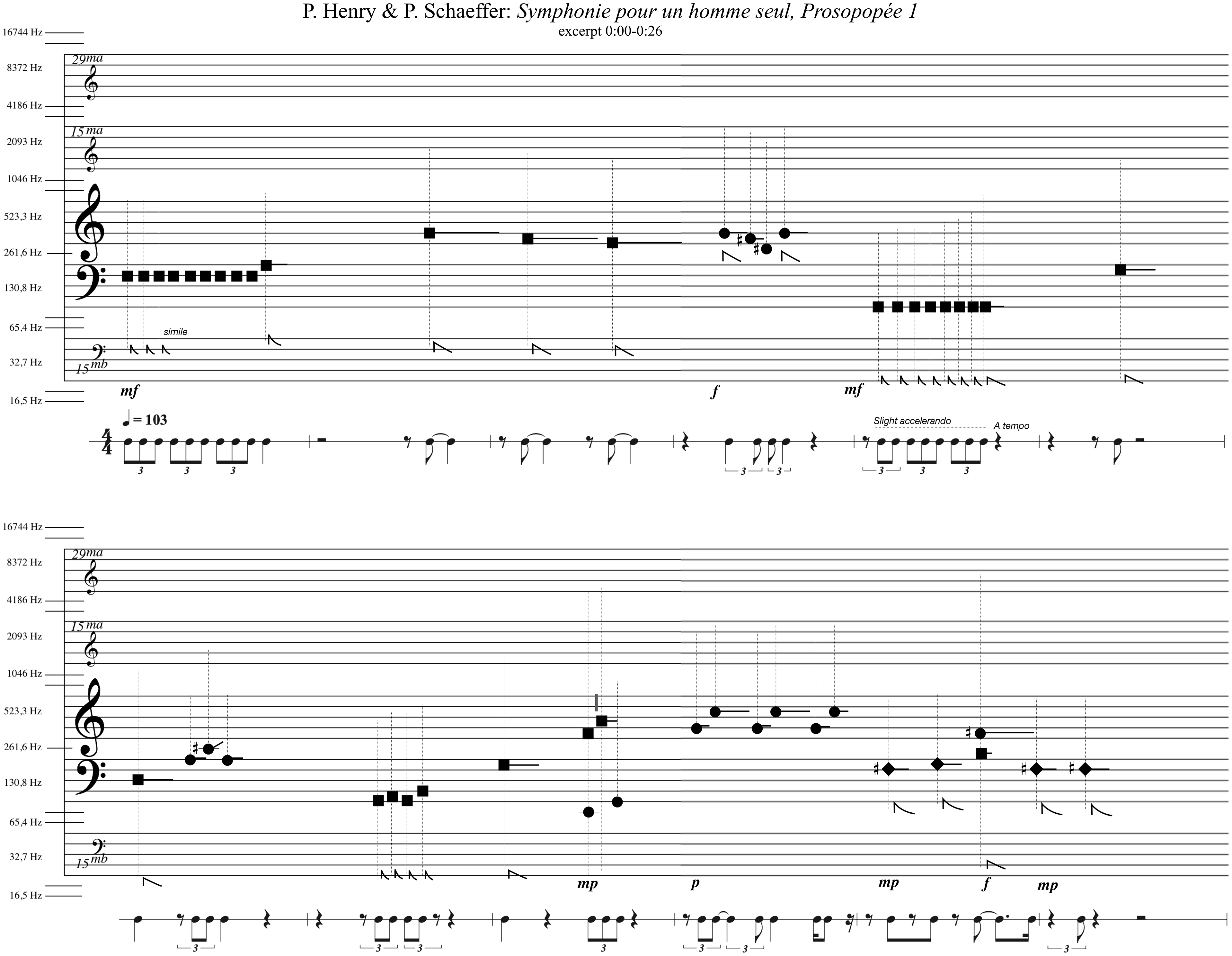
Figure 7. Sound notation transcription of excerpt from Prosopopée 1 from Symphonie pour un homme seul (Henry Reference Henry2000).
4.1. Pierre Henry and Pierre Schaeffer: Prosopopée 1 from Symphonie pour un homme seul (1950)
The first transcription is of a classic musique concrète work from 1950 with no synthesised sounds. The introduction of Prosopopée 1 from Symphonie pour un homme seul (Henry Reference Henry2000) presents a variety of sound sources, most notably repetitive phrases of percussive sounds with small timbral variations and cut-out voice recordings. Figure 7 shows my sound notation transcription of the first 26 seconds of the piece. The trancription shows how phrases appear and how they change as they reappear. The indicators of spectral width show that here is not much significant high frequency range spectral energy. It is clear from the transcription that the traditional musical parameters, pitch, rhythm and dynamics, are important.
4.2. Karlheinz Stockhausen: Kontakte (1960)
Kontakte is interesting from a timbral point of view for many reasons, one of which is how Stockhausen works with degrees of transformation of musical parameters as a forming principle (Brandorff and La Cour Reference Brandorff and La Cour1975). The transcribed excerpt seen in Figure 8 covers 11′19,3″ to 11′35,2″ of the tape part of Kontakte (according to the original score’s timeline). The work exists as a standalone fixed media work and as a mixed work for piano, percussion and tape. The transcription in Figure 8 shows how Stockhausen combines different kinds of spectra, also working with changes in granularity. It was transcribed on two parallel staff systems because of the many layers of sound. The upper system shows the development of pitched sounds, ending with a long iterated pitched sound with narrow spectral width and variable iteration speed indicated in hertz. The lower system shows the amplitude variation of a long, soft, sustained dystonic sound, along the two occurrences of iterated complex sounds with relatively dense spectra. Because of the importance of the iteration for the timbral character of this passage, fairly precise frequency values indicate the speed of the iterations. Spatialisation is also important in this quadraphonic work. However, this aspect was not covered by the transcription, focusing mainly on the timbre structure.

Figure 8. Sound notation transcription of excerpt from Kontakte (Stockhausen Reference Stockhausen1992).
An important aspect of Kontakte is its detailed realisation score (Stockhausen Reference Stockhausen1995), created by the composer. This score allows for the two musicians to synchronise their performances with the tape part but it also sheds light on the timbral structure of the composition as envisioned by the composer, though it does not allow for exact readings of parameters. Even though my sound notation transcription was made without consulting the score, they have similarities. Stockhausen seems to have positioned the symbols for his pitched sounds with vertical distances compatible with staff notation, and he too imagined the repeated sound grains mainly as elements of continuous sounds (notated with smooth zigzag lines) rather than separate sound objects.
4.3. Ligeti: Artikulation (1958)
Finally there is a transcription of the time 0′30″ to 0′40″ of Ligeti’s Artikulation from 1958 (Ligeti Reference Ligeti1988). Besides being a classic electroacoustic musical work, it is also known for its graphical score (Wehinger Reference Wehinger1970), which was not part of the composition process but made later as a listening score distributed with a recording of the work. Although Wehinger’s symbols constitute a systematic categorisation of timbre, they were only designed to describe this particular musical work, and they are expressed in terms of the sounds’ (assumed) production. Also, the symbols’ placements in the score only approximate register relations and durations. Therefore, my transcription in Figure 9 is dissimilar to the corresponding passage of the listening score. The challenge was to get the pitch and time information right., For this transcription, reverb indications were used because of how the reverberation effects articulate the phrases.
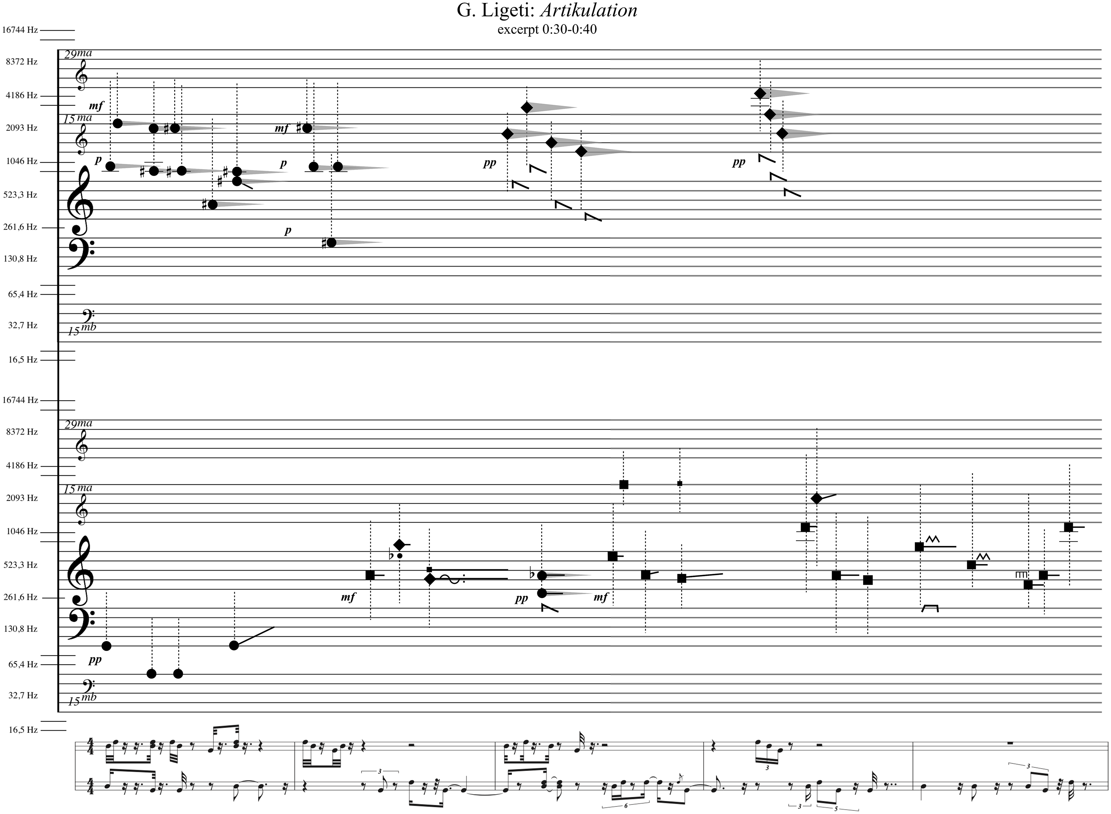
Figure 9. Sound notation transcription of excerpt from Artikulation (Ligeti Reference Ligeti1988).
4.4. About the transcripts
Electroacoustic music does not necessarily need scores for its conception. Yet, there are great pedagogical benefits of having the realisation and listening scores for Stockhausen’s and Ligeti’s works. What my notation system contributes is the possibility to place the transcriptions side by side and make reasonable comparisons. Also, the fact that the symbols correspond to measurable timbre parameters makes it possible to recreate the music based on its notation. This has already been tried with students at the Royal College of Music in Stockholm with rewarding results. Since these transcriptions did not contain spectral references, there is of course much room for interpretation, so even perfect realisations of the transcribed scores will not be identical to the originals.
5. EVALUATION: EMPIRICAL STUDIES
In order to test the intuitiveness of the system, two studies were conducted: one small pilot study with a limited number of participants, and one online survey. Both studies were made with listeners familiar with traditional music notation and/or electroacoustic music.
5.1. Sound and notation examples
In both studies the same five examples were used: each example consisted of a sound file and its two possible notated transcriptions, labelled A and B (see Figure 10). One was the correct notation and the other was a slightly altered version of the correct notation. Examples were designed to test the intuitiveness of different aspects of the representation system with regard to timbre, including the use of non-pitched spectrum symbols (diamond- and square-shaped note heads) with a traditional staff-system. For the spectrum reference example (Example 3), a recorded piano tone was used for the sound file, with its characteristic attack removed and its amplitude envelope modified so that only the spectral qualities of the sustained piano tone remained. The test was conducted without any introduction to the symbols and functionality of the notation system.
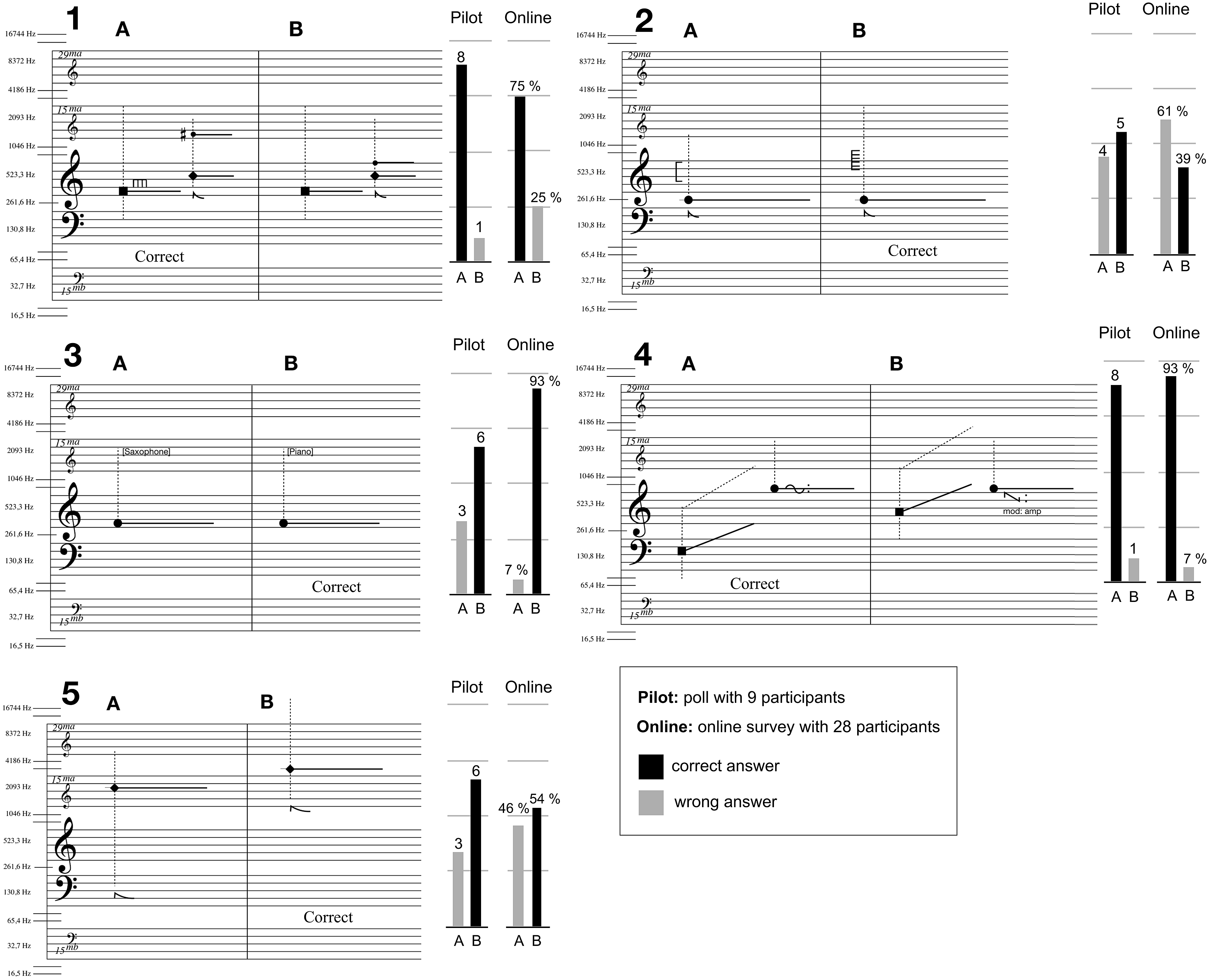
Figure 10. The notation and results of the two empirical studies. The participants were presented with sounds and were asked whether notation A or B best describes what they heard. The result of the pilot study with nine participants is shown as numbers of participants while the result of the follow-up online survey with 28 participants is shown as percentage values.
5.2. Pilot study
Nine participants took part in the pilot study, conducted in the Zoom conferencing system (1 female, 8 male; average age 42, standard deviation 6.67). Six participants had professional music training and three had some musical training. Eight were listening through high-quality headphones and one was using medium-quality headphones. The participants were to various degrees familiar with this research but had not seen or heard the examples used in this test before. The examples were presented to the participants in a particular order, one to five, and each sound file was played three times. The participants were then asked to ‘Choose the notation you believe best describes the sound you heard’. The Zoom polling function was used to collect their answers.
Figure 10 shows the A and B notation options together with the results from both studies. In the pilot study, a majority of the participants selected the correct notation for all five examples. Examples 1 and 4 stood out with eight out of nine participants selecting the correct notation. The most significant difference between these two examples and the other three is that they include two sound objects instead of one. This is relevant since we can better judge a sound parameter value in relation to another value. A difference between Examples 1 and 4 is that for Example 1, the notation options contain differences for the vertical positions of pitched elements, while in Example 4, the notation options contain differences for the vertical positions of complex spectra (indicating spectral centroid positions). Example 2 only had five out of nine participants selecting the correct notation indicating a possible problem with the intuitiveness of this notation of spectral density.
5.3. Online study
For the second study, 28 participants (5 female, 23 male; average age 52.86, standard deviation 9.58) took part in an online survey with the same five examples as in the pilot study. Regarding their music reading proficiency, 20 participants had professional level, seven had some skill and one had none. Regarding music technology/electroacoustic music proficiency, 19 had professional level, eight had some skill, and one had none. This time, the order of the examples was randomised and the questions were not numbered. The participants could listen to the sounds as many times as they wanted. But the same question was asked as in the pilot study, whether notation A or B best describes the sound they heard.
Comparing the test performance between age groups 25–39, 40–9, 50–9 and 60–85 using one-way ANOVA showed no significant influence of age, F(3,24) = 0.61, p = .61. There were no significant differences in performance either between male participants (M = 3.57, SD = 0.9) or female (M = 3.4, SD = 0.55); t(26) = 2.26, p = .60, between participants with some music reading skill (M = 3.29, SD = 0.49) and professional level (M = 3.70, SD = 0.86); t(25) =2.09, p = .14, or between participants with some skill in music technology/electroacoustic music (M = 3.75, SD = 0.71) or professional level (M = 3.42, SD = 0.88); t(25) = 2.11, p = .32. Note that the two latter tests were performed on the 27 answers divided between the some skill and professional level categories, excluding the single answers specifying no skill.
On the whole, the online study reinforced the results from the pilot study (see Figure 10). Again, Examples 1 and 4 showed good results: 75 per cent and 93 per cent correct answers. Example 3, about spectral references, also received a high amount of correct answers (93 per cent). Example 5, mainly about the spectral width of inharmonic spectra, had somewhat worse results (54 per cent) than in the pilot. The online study confirmed a lack of intuitiveness for relating a (pitched) sound to my indicator for spectral density with only 39 per cent choosing the right symbol.
The generally good results of the two studies suggest that placing new spectral symbols over a staff system along a frequency axis is indeed intuitive. In neither study did the participants receive any explanation of the notation system before answering the questions. Example 1 benefits from the two notation options having pitched components notated over a traditional staff system. However, pitched components are not easy to identify without reference tones, as evidenced by the weak results for Example 5 (which was about identifying the notation for a dystonic (inharmonic) sound object and its spectral width in a high register). The somewhat poor result for Example 5 shows the difficulty involved in identifying spectral bandwidths without a reference. Also, pitches at 3.5 kHz are not common in acoustic music (coinciding with the highest register of the piccolo flute). A major difference between the two options in Example 4 is the spectral width parameter change for a complex (not harmonic) spectrum category. Here, the pitch position of the pitched sound is of no help other than to act as a reference tone for the centroid of the complex spectrum since the pitch is the same for both notation options. I did not expect that Example 3 would provide such good results, considering that it was only the sustained timbre of the piano that the participants could hear. The characteristic attack and amplitude envelope had been removed. However, the fact that the option was a saxophone spectrum may have helped in deciding in favour of the piano. The study confirmed a lack of intuitiveness for relating a given sound to my indicator for spectral density with only 39 per cent choosing the right symbol. This was to be expected since spectral width is not commonly encountered as a musical parameter, even in electroacoustic music. This result has made me reconsider how to use the symbol; initially I intended for it to be dependent on the spectrum category, since maximum partial densities are different for the three categories. However, the confusion regarding a high spectral density indicator for a harmonic spectrum could in part be explained by the listeners not perceiving this density, particularly in the context of the survey that contained several complex and dystonic sound objects with more densely populated spectra.
6. DISCUSSION AND CONCLUSIONS
A major concern when designing musical notation is the level of detail with which a parameter is to be described. Charles Seeger showed effectively how the notation of pitches in traditional notation differs from the performed pitch contour in a sung melody (Seeger Reference Seeger1958). This reduction is true for all main parameters of traditional music notation. Similarly my notation of the spectral qualities of timbre were not developed to describe the full scope of a spectrum as it is experienced, but rather to provide musically meaningful tools for introducing timbre as a (multidimensional) musical parameter alongside already established parameters. Inevitably this means some form of reduction of information.
Timbre remains an elusive musical parameter, the complexity of which depends on its multidimensionality and relation to sound identity and source recognition. Adding to the confusion, the term ‘timbre’ is used sometimes to indicate only the spectral characteristics of a sound and in other cases the totality of a sound’s character.
Symbols borrowed from Thoresen and Hedman’s analysis notation, developed to be relevant for the study of musical structures, were adapted to signify acoustic properties relevant for the perception of timbre. Focusing on spectral aspects of timbre in this context, the notated features are: spectrum category, spectral width, centroid and density, spectral components and timbre reference. Of these, the spectrum category and the timbre reference are of particular importance. The category is important because of how a particular sound object’s origin in a given spectrum category affects how we perceive spectral changes to this sound object. The reference is important because it relates to several spectral qualities at once, also acknowledging timbre’s function as a source for sound recognition. Notation for energy articulation, the spectral morphology, is also part of my research but is beyond the scope of this text.
The notation was demonstrated in transcripts of excerpts of pioneer work in electroacoustic music, and readers familiar with these works can judge the suitability of representing these excerpts in this fashion. Such transcripts open up new possibilities for the re-interpretation of non-score-based work in the same way that pitch-based improvisations are sometimes transcribed and re-interpreted. While spectrograms already made it possible to compare musical works based on their spectral information, they lack auditory stream segregation, as well as indications of perceptually relevant parameters that may be in focus in the composition. Also, neither pitch nor rhythm are satisfactorily represented in spectrograms. However, spectrograms can be valuable as complementary sources of information, which is why it is commonly used as a backdrop for software-based electroacoustic music analysis as in the analysis software Acousmographe and eAnalysis.
In general the listener tests showed that the combination of spectral notation symbols and traditional notation features was intuitive. It was easier to understand the notation examples with two sound objects than those with one. Relating the high spectral density of a pitched sound to the corresponding high density symbol showed to be difficult and this result has changed the way I use this indicator in relation to the three spectrum categories.
The success of the notation depends on its usability for both composition and analysis. So, while it would be easier to navigate the already complex field of timbre research either as a concept of human perception or as something to be retrieved from a physical or electronic sound source, as a composer I am very much relying on tools that firmly place themselves midway between the two. The goal is a notation that serves imagination, perception and communication.


 Open access