


Introduction
While the fossil record provides a unique window into past life on Earth, it is well known that it is both pervasively and nonuniformly biased (Raup Reference Raup1976; Koch Reference Koch1978; Foote and Sepkoski Reference Foote and Sepkoski1999; Alroy et al. Reference Alroy, Marshall, Bambach, Bezusko, Foote, Fursich, Hansen, Holland, Ivany, Jablonski, Jacobs, Jones, Kosnik, Lidgard, Low, Miller, Novack-Gottshall, Olszewski, Patzkowsky, Raup, Roy, Sepkoski, Sommers, Wagner and Webber2001; Allison and Bottjer Reference Allison and Bottjer2011a). Geologic, taphonomic, and anthropogenic biases (such as the amount of available fossiliferous rock for sampling, variation in fossilization, and the degree to which the available rock record has been sampled) skew or remove information from the fossil record, leaving the remaining catalog of data uneven and incomplete. Although biomineralized remains have an increased preservation potential compared with soft-bodied tissues (Allison Reference Allison1988; Briggs Reference Briggs2003), they are still influenced by various geologic and taphonomic processes (Kidwell and Jablonski Reference Kidwell, Jablonski, Tevesz and McCall1983; Kidwell and Bosence Reference Kidwell, Bosence, Allison and Briggs1991; Kidwell and Brenchley Reference Kidwell and Brenchley1994; Best Reference Best2008; Hendy Reference Hendy2011). Shelly marine faunas are especially susceptible to misrepresentation due to preferential dissolution of biogenic carbonate polymorphs. It is well established that aragonite, a polymorph of CaCO3 found within the biomineralized shells of many invertebrates, dissolves more rapidly than the more common form of CaCO3, calcite, and at a higher pH (Canfield and Raiswell Reference Canfield, Raiswell, Allison and Briggs1991; Tynan and Opdyke Reference Tynan and Opdyke2011). While both polymorphs can be destroyed by adverse conditions near the sediment–water interface (Best and Kidwell Reference Best and Kidwell2000) and the effects of dissolution can vary between fauna (due to microstructure surface area, morphology, and shell organic content; Walter and Morse Reference Walter and Morse1984; Harper Reference Harper2000; Kosnik et al. Reference Kosnik, Alroy, Behrensmeyer, Fürsich, Gastaldo, Kidwell, Kowalewski, Plotnick, Rogers and Wagner2011), it is still the case that aragonitic shells are more likely to dissolve than calcitic remains (Brett and Baird Reference Brett and Baird1986). As mineral composition of mollusks is usually conserved at the family level (Carter Reference Carter and Carter1990), this has the potential to skew the record of molluscan diversity and trophic structure through time (Cherns and Wright Reference Cherns and Wright2000; Wright et al. Reference Wright, Cherns and Hodges2003; Cherns et al. Reference Cherns, Wheeley and Wright2011) and negatively affect subsequent work that relies on the relative abundance and distribution of shelly marine fauna (Kidwell Reference Kidwell2005). Cherns and Wright (Reference Cherns and Wright2000) argued that early-stage dissolution could be substantial and referred to the phenomenon as the “missing mollusk” bias. Subsequent work at a multitude of temporal and spatial scales (Wright et al. Reference Wright, Cherns and Hodges2003; Bush and Bambach Reference Bush and Bambach2004; Kidwell Reference Kidwell2005; Crampton et al. Reference Crampton, Foote, Beu, Maxwell, Cooper, Matcham, Marshall and Jones2006; Valentine et al. Reference Valentine, Jablonski, Kidwell and Roy2006; Foote et al. Reference Foote, Crampton, Beu and Nelson2015; Jordan et al. Reference Jordan, Allison, Hill and Sutton2015, Hsieh et al. Reference Hsieh, Bush and Bennington2019) has debated the magnitude of this bias; however, there is a broad agreement on the potential for dominantly aragonitic shells to suffer greater postmortem diagenetic destruction in the taphonomically active zone (TAZ) (Davies et al. Reference Davies, Powell and Stanton1989; Foote et al. Reference Foote, Crampton, Beu and Nelson2015). While the effect of dissolution on the global macroevolutionary record of mollusks has been found to be limited, possibly due to the potential of aragonite to recrystallize to calcite (Kidwell Reference Kidwell2005; Paul et al. Reference Paul, Allison and Brett2008; Jordan et al. Reference Jordan, Allison, Hill and Sutton2015), it is conceivable that local or regional conditions could severely impact perceived patterns of biodiversity in restricted areas (Bush and Bambach Reference Bush and Bambach2004). In a regional study of Cenozoic mollusks, Foote et al. (Reference Foote, Crampton, Beu and Nelson2015) found evidence to suggest that aragonite dissolution was both enhanced in carbonate sediments and insignificant within siliciclastic sediments, with similar preservation potential of aragonitic and calcitic fauna within the latter. They further emphasized the fact that scale is an important factor in determining the observable impacts of aragonite dissolution, which will strongly vary between local (potentially consisting of an individual bed), regional, and global studies. However, to date, research has focused on assessing the influence of aragonite bias on temporal trends of biodiversity and has ignored the potential for direct spatial expression.
Early-stage dissolution occurs within modern environments as a result of microbially mediated reactions increasing local acidity (Walter et al. Reference Walter, Bischof, Patterson, Lyons, O'Nions, Gruszczynski, Sellwood and Coleman1993; Ku et al. Reference Ku, Walter, Coleman, Blake and Martini1999; Sanders Reference Sanders2003). Bacterially mediated decay of organic material within the upper sedimentary column occurs in a series of preferential redox reactions. By-products of these reactions, such as solid-phase sulfides from sulfate reduction and CO2 from aerobic oxidation, result in changes to local pore-water saturation of calcium carbonate (Canfield and Raiswell Reference Canfield, Raiswell, Allison and Briggs1991; Ku et al. Reference Ku, Walter, Coleman, Blake and Martini1999). Additionally, oxidation of H2S above the oxycline increases acidity at that boundary; if this occurs at the sediment–water interface, it can adversely affect the preservation of shelly marine fauna (Ku et al. Reference Ku, Walter, Coleman, Blake and Martini1999). As such, dysoxic sedimentary environments might have a predisposition for dissolution of biogenic carbonate and enhance the effect of the “missing mollusk” bias (Jordan et al. Reference Jordan, Allison, Hill and Sutton2015). Epicontinental seas, marine water bodies that form by the flooding of continental interiors, are especially prone to strong water-column stratification and sea-level variation and have a predisposition to seasonally anoxic or dysoxic conditions (Allison and Wells Reference Allison and Wells2006; Peters Reference Peters2009). As such, they have the potential to be more prone to both preferential aragonite loss and preservation than modern oceans. Cherns et al.’s (2011) model for taphonomic gradients of aragonite preservation along a shelf-to-basin transect can be readily applied to epicontinental sea settings (Fig. 1). If we assume the center of a seaway was stratified with at least a seasonally anoxic basin floor, we would expect enhanced dissolution to occur in the seaway margins, likely in the mid- to outer-shelf setting (Cherns et al. Reference Cherns, Wheeley and Wright2011). We would expect to see enhanced preservation in the anoxic basin center, as an aragonitic skeleton residing on the surface sediment in an anoxic water column would not be susceptible to dissolution from H2S oxidation (Jordan et al. Reference Jordan, Allison, Hill and Sutton2015); however, we would not expect to see abundant benthos in such a setting because of bottom-water toxicity. It is apparent this could result in spatially expansive zones with conditions predisposed for heightened aragonite dissolution and preservation (Fig. 1); it is important to note that we do not expect all aragonitic fauna to be missing from any region of the seaway—merely that a lower relative proportion of aragonitic mollusks be found, due to a reduced probability of an individual site recording their occurrence. How these hypothesized basin-margin to basin-center zones could influence long-term patterns of mollusk distribution, preservation, and recovery remains to be examined. As epicontinental seas contain the majority of our Phanerozoic fossil record (Allison and Wells Reference Allison and Wells2006), it is imperative that we understand systematic biases that may specifically affect these settings.
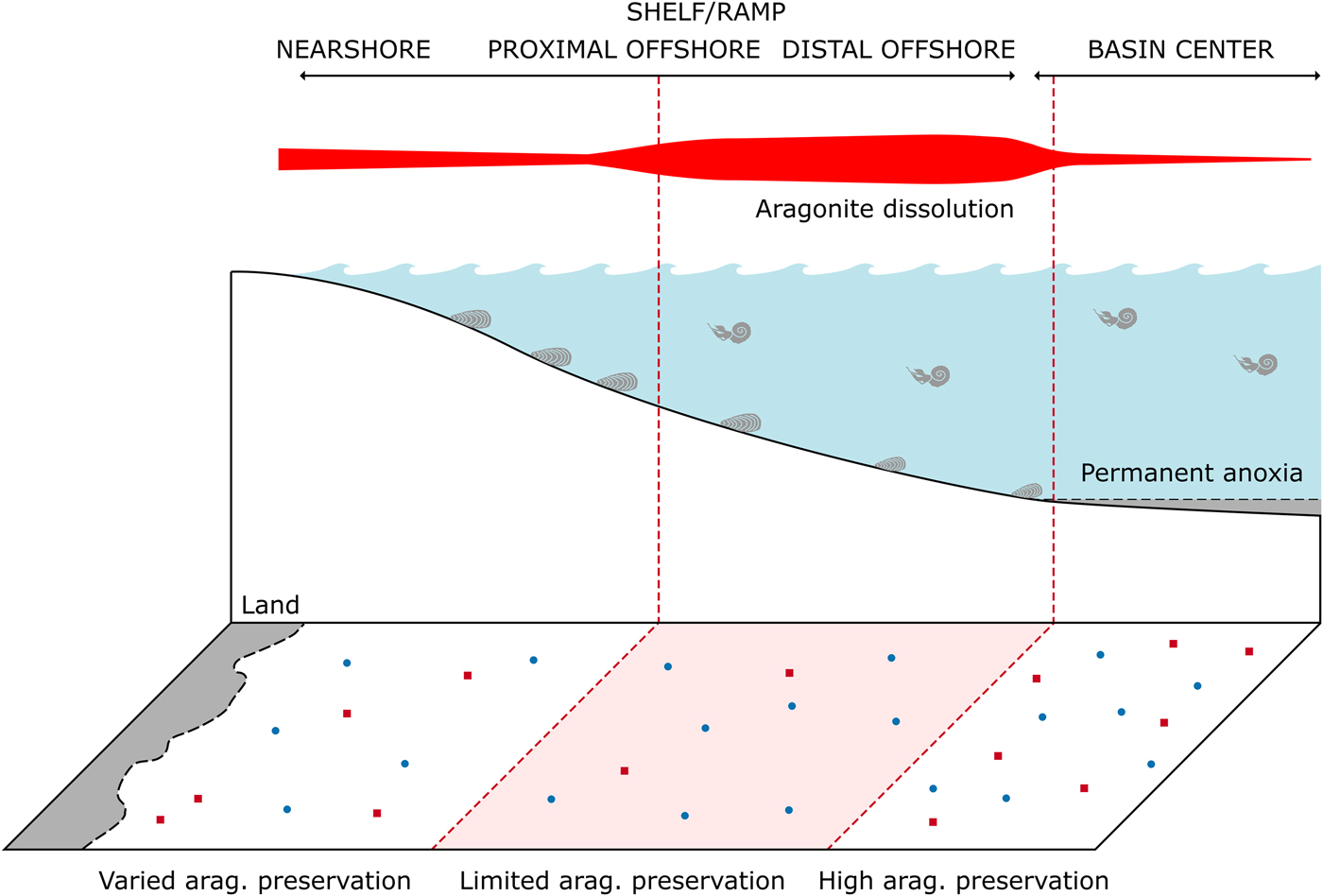
Figure 1. Diagram showing potential model of spatial aragonite bias within the Western Interior Seaway. Within the outer shelf, preferential dissolution of aragonitic fauna is common, which has the potential to be expressed spatially. Within the basin center, anoxia limits benthic organism development, but allows for preservation of aragonitic material. Modified after Cherns et al. (Reference Cherns, Wheeley and Wright2011).
Here we present a spatial investigation of aragonite dissolution within the Late Cretaceous Western Interior Seaway (WIS) of North America, using sampling probability estimates and multiple logisitic regression to evaluate patterns of spatial distribution in preserved calcitic and aragonitic fauna. We address two key questions: (1) Does aragonite bias exhibit systematic spatial variation across the seaway, and (2) if so, does this influence perceived patterns of diversity?
Materials and Methods
Time Intervals and Paleogeography
The two stratigraphic intervals or time slices (Cenomanian–Turonian and early Campanian) were selected: (1) because of purported dysoxic conditions within their duration; and (2) due to their differences in environment, oceanography, and preserved lithology, allowing for comparison of taphonomic regimes. The first interval covers the Cenomanian/Turonian boundary, spanning the Dunveganoceras pondi Zone to the Collignoniceras woollgari Ammonite Zone (~94.7–93 Ma) (Cobban et al. Reference Cobban, Walaszczyk, Obradovich and McKinney2006). The second interval spans the early Campanian, from the Scaphites leei III Zone to the Baculites obtusus Ammonite Zone (~83.5–80.58 Ma) (Cobban et al. Reference Cobban, Walaszczyk, Obradovich and McKinney2006). The geologic context of stratigraphic intervals is detailed in Supplementary Information 1.
A global atlas of 1:20,000,000 scale paleogeographic maps, compiled by GETECH PLC, formed the basis for new regional-scale, high-resolution interpretations for the selected time intervals. The original paleogeographic maps (Markwick Reference Markwick, Williams, Haywood, Gregory and Schmidt2007) are underpinned by the GETECH plate model (v. 1), which is outlined further in Supplementary Information 1. High-resolution mapping involved synthesis of stratigraphic, sedimentologic, and paleontological information to produce 1:5,000,000 scale paleogeographies with suggested paleobathymetry. A full list of decisions on paleogeographic reconstructions and key references for each time interval are provided in Supplementary Information 1.
Landward-to-basinward arrangements of a priori binned zones for each time slice were based on average paleobathymetry (Fig. 2). Bathymetric reconstructions were divided into four bins, each of which covers a specific interpreted depth range: nearshore (<50 m), proximal offshore (50–100 m), distal offshore (100–150 m), and basin center (>150 m). These designations were based on the previously constructed paleobathymetry for the WIS produced by Sageman and Arthur (Reference Sageman, Arthur, Caputo, Peterson and Francyzk1994), but match the paleobathymetry in our new maps and represent a reasonably high resolution without being compromised by large changes in shoreline position within our chosen time slices.
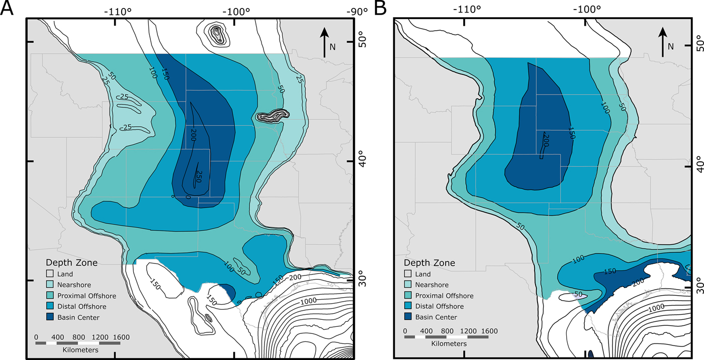
Figure 2. Paleogeographic zoned maps of the Western Interior Seaway used in this study. Depth-based zones are designated as nearshore, proximal offshore, distal offshore, and basin center (Fig. 1). A, Paleobathymetric map of the Cenomanian–Turonian; B, paleobathymetric map of the early Campanian.
Distance from paleoshoreline zones (Supplementary Fig. S1) were constructed based on 50 km intervals from the time-averaged paleoshoreline position until reaching the basin center, with number of occurrences, collections, and total outcrop area plotted per zone. These were generated by constructing a fishnet of points in ArcGIS (ESRI 2010) using the Fishnet tool, which were selected by the Select By Location tool with increasing distance in 50 km intervals from the paleoshoreline: the positions of the most-basinward selected points were used for the bin boundary. Results for depth zones are used in the main body of this paper; distance from paleoshoreline zones are available in Supplementary Information 1 and Supplementary Figures S2, S4, S6, and S7.
Fossil Data Set
A presence-only fossil occurrence data set of bivalve and ammonite taxa was produced for the selected stratigraphic intervals, collated from personally provided digitized collections from the U.S. Geological Survey (USGS) and Smithsonian Museum of Natural History (NMNH) and downloads from the Paleobiology Database (PBDB; http://paleobiodb.org) and iDigBio (http://www.idigbio.org). Each occurrence includes taxonomic and geographic locality data, an associated collection with lithologic and geologic information, and modern latitudinal and longitudinal coordinates. Data were extensively screened for problematic records and to ensure taxonomic validation (see Supplementary Information 2 for the latter).
The resultant Cenomanian–Turonian data set contains 5867 occurrences from 2409 localities, with 207 genera, 1549 species, and 3886 specimens identifiable to the species level. The early Campanian data set comprises 2544 occurrences from 1186 localities, recording 163 genera, 1405 species, and 1405 specimens identifiable to the species level. Generic-level taxonomic diversity was used for all tests; species-level results can be found in Supplementary Information 1 and in Supplementary Figures S3–S6. Full information regarding downloads, sources, and screening of data can be found in Supplementary Information 1, and the full data set can be found in Supplementary Information 2.
Mineralogy
Bivalve shells are a composite of layered mineral crystallites, which are sheathed by a refractory organic matrix of fibrous protein (Taylor Reference Taylor1969). As these mineral layers can be composed of both calcite and aragonite, variation in overall mineral composition must be taken into account when assigning a predominant mineralogy to a specific bivalve genus. Different scoring mechanisms have been adopted by previous workers to address this issue. Kidwell (Reference Kidwell2005) used a five-point decimal scoring system from entirely aragonitic (1) to entirely calcitic (3), with three permutations of mineralogy between. Crampton et al. (Reference Crampton, Foote, Beu, Maxwell, Cooper, Matcham, Marshall and Jones2006) adopted a simple and effective system of counting organisms as calcitic if they contained a calcitic element that would allow them to be identified to the species level. We utilize a combination of these approaches—organisms were scored using the system of Kidwell (Reference Kidwell2005) to maintain the maximum amount of data, but simplified into binary categories afterward based on whether they contained sufficient calcitic parts to enhance preservation potential. Note that we have not included either the inner myostracal layer or periostracum in our assignments of mineralogy.
Information on shell composition was predominantly gathered from a personally provided data set from S. Kidwell (Kidwell Reference Kidwell2005), with additional information from studies by Taylor (Taylor Reference Taylor1969; Taylor and Layman Reference Taylor and Layman1972), Majewske (Reference Majewske, Cuvillier and Schürmann1974), Carter (Reference Carter and Carter1990), Schneider and Carter (Reference Schneider and Carter2001), Lockwood (Reference Lockwood2003), Hollis (Reference Hollis2008), and Ros Franch (Reference Ros Franch2009) and many papers focused on single genera or families. For genera for which information regarding shell mineralogy was not available, composition was assigned based on the dominant mineralogy of the family, as composition is highly conservative both among species within a genera and among genera within a family (Taylor Reference Taylor1969). In total, 124 bivalve genera were assigned a mineralogy, of which 41 (~33%) were achieved using familial relation (Supplementary Information 2).
Life Habits
Life habits of bivalves were assembled to allow additional interrogation and interpretation of environmental and sampling regimes. Life habits were separated into the following categories: relation to substrate, mobility, and diet. Data for each genus of bivalve were primarily gathered from the NMiTA Molluscan Life Habits Database (Todd Reference Todd2017) and the PBDB, with further data collected from the wider literature (Supplementary Information 2).
Outcrop Area
Relevant rock outcrop area was plotted per zone to evaluate broader-scale bias influencing patterns of fossil distribution. Outcrop areas for the selected time slices were generated by combining statewide digitized geologic maps from publicly available USGS downloads and selecting shape files that matched formations found within those time slices. Some state surveys grouped relevant formations with other partially contemporaneous formations that spanned multiple stages: we chose to include these designations in order to present the maximum possible sampling extent in terms of outcrop area. Outcrop was projected in ArcGIS (ESRI 2010) using the USA Contiguous Albers Equal Area conic projection, to minimize distortion of distances. Outcrop areas per zone were created by using the Intersect tool in the Geoprocessing toolbar in ArcGIS, and area (km2) calculated using the Calculate Geometry function in the attribute table. Outcrop was split into depth zones by using the Intersect tool in ArcGIS (ESRI 2010). Outcrop area for each zone was calculated by summing the total area of all outcrop polygons within that zone. Collections per zone were counted by exporting occurrences selected in zones in the seaway as shapefiles, then using the arcgisbinding package to view and organize the data in R v. 3.0.2 (R Core Team 2017).
Dominant Lithology
Each collection was assigned a dominant lithology to allow for comparative testing. If these data were not available, a lithology was assigned from the dominant lithology of the formation, with reference to USGS formation records. Collections were assigned one of the following lithologies (primarily based on original USGS records): siliciclastic mudstone, siliciclastic siltstone, siliciclastic sandstone, conglomerate, ironstone, calcareous mudstone and siltstone, marl, calcarenite, limestone, and chalk.
Range Size
If the presence of preferentially destructive zones is affecting the spatial distribution of aragonitic fauna, we might expect to see overall smaller range sizes for aragonitic organisms compared with calcitic organisms (Fig. 3). As such, range-size estimates were produced for calcitic and aragonitic bivalves and compared to test whether aragonite bias influenced perceived range of aragonitic organisms. Note that ammonites were excluded from this test due to the difference in life habit between them and bivalve fauna: ammonites have a pelagic to nektono-benthic mode of life (Ritterbush et al. Reference Ritterbush, Hoffmann, Lukeneder and De Baets2014), while bivalves are predominantly epifaunal and infaunal.
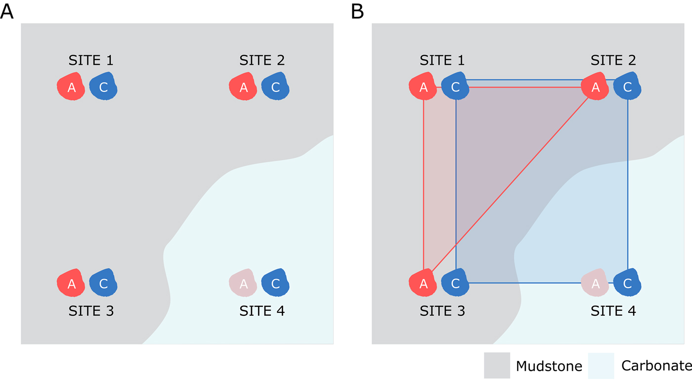
Figure 3. Diagram showing potential model of apparent range-size reduction due to spatially variable aragonite preservation. Assuming that calcitic and aragonitic species of bivalve were both living at four separate localities, but aragonitic dissolution strongly influenced one of those locations (A), the resulting convex hull for the aragonitic fauna drawn from surviving fossil occurrences would likely be smaller than that for the calcitic organisms (B).
Geographic locality data for the selected fauna were visualized in ArcGIS (ESRI 2010). Faunal occurrences were paleo-rotated using the Getech Plate Model to match the paleogeography of the appropriate stages of the Late Cretaceous. This ensures that tectonic expansion and contraction of the North American Plate from the Mesozoic to the Recent has a negligible effect on propagating estimation error in range-size reconstructions. Fossil occurrences were projected into ArcGIS using the using the USA Contiguous Albers Equal Area conic projection. A 10 km buffer was additionally applied to each occurrence point to control for any error in paleogeographic or present position of fauna. ArcGIS (ESRI 2010) was then used to construct convex-hull polygons for each taxon, and the Spatial Analyst tools from this software calculated the area of each reconstructed polygon. We did not account for landforms within the ranges of any organisms, and thus ignored their area when calculating overall area of ranges. Several vertices for range-size polygons appeared on what is classified as land within our paleogeographies; due to rapid changes in shoreline position within the WIS, we decided to keep using these fauna for range-size estimations. Myers and Lieberman (Reference Myers and Lieberman2011) showed that relative range sizes for vertebrates in the WIS were not overly affected by resampling occurrence points—consequently, we have not carried out a similar test for this study. Comparisons between the ranges of aragonitic and calcitic fauna were carried out using the Wilcoxon-Mann-Whitney test with continuity correction (Brown and Rothery Reference Brown and Rothery1993). Geographic range data for all applicable taxa are provided in Supplementary Information 2.
Sampling Probability and Multiple Logistic Regression
To further observe differences between aragonitic and calcitic organisms throughout the seaway, we employed a modified version of the sampling probability method used by Foote et al. (Reference Foote, Crampton, Beu and Nelson2015; after Foote and Raup Reference Foote and Raup1996). In this method, the sampling probability of a time bin was generated by compiling a list of all fauna with originations older than that bin and extinctions younger than that bin, and then dividing the total number of species found within the bin by that figure. This allows for a sampling probability to be estimated on a per-bin, per-group basis. Here we devised three variants on this method for application in the spatial realm. It should be made clear that the modified methods used in this work come with the caveat that in the spatial realm it is impossible to know whether a species was present in a precise location in the past: for instance, if zones A, B, and C are designated with increasing distance away from a paleoshoreline, it cannot be assumed that because an organism exists in zones A and C that it was ever present in zone B. Consequently, the probabilities generated from the methods described below are relative and cannot be taken as “true” probabilities. However, the methods used were designed to be as inclusive as possible and to deliver a strongly conservative estimate of true sampling probabilities between groups; these methods therefore provide a useful estimate on the relative likelihood of sampling aragonitic or calcitic fauna. Furthermore, sampling probabilities through time based on regional studies such as those used by Foote at al. (Reference Foote, Crampton, Beu and Nelson2015) rely on the assumption that groups were not genuinely absent from the study region at a particular time and that other geographic variables do not have an effect—as such, the use of these metrics to evaluate the distribution of fauna across the WIS is validated.
Three methods were devised for dealing with the issue of unknown “correct” distribution of species across the seaway and to correct for differences in the number of collections between zones: method 1 finds two bins either side of the current bin and generates a list of the total number of possible species across those five bins; method 2 finds all formations that appear in the selected bin that contain specimens of the selected group (e.g., calcitic bivalves), and then finds the total number of species for that group from those formations; method 3 finds all formations in the current bin and the two adjacent bins that contain specimens of the selected group, and subsequently finds the total number of species from those formations. For all three methods, the total number of sampling opportunities per bin was generated by multiplying the number of potentially recoverable species by the number of collections to standardize for differences in collecting intensity. The low number of depth-based bins could potentially result in flattening the curve of sampling probability using method 3, and thus method 2 is employed in the main body of this paper for depth-based results.
To determine the primary controls on sampling probability between the two stages, we used multiple logistic regression, coding sampling opportunities as the response variable and mineralogy, lithology, life habits (mobility, relation to substrate, and feeding style), and depth zone as the predictor variables. Multiple logistic regression allows for the use of binomial nominal values by using the odds ratio, a measure of the relationship between the odds of an outcome, in this case sampled (1) or not sampled (0), along with multiple potentially explanatory ecological or physiographic variables. A full model is generated that incorporates all potential variables, and a null model is defined that includes none. Stepwise addition or deletion from the null or full models, respectively, and analysis in the change of likelihood and of respective Akaike information criterion (AIC) scores contribute to a final predictive model of explanatory variables and respective statistical significance.
Sampling opportunities were tabulated as the presence or absence of each recoverable genus per collection, per depth zone. Each sampling opportunity was assigned a lithology based on collection lithology, as well as all ecological attributes related to that genus. To test for multicollinearity between variables, correlation tests were run using Spearman's rank correlation using the Performance Analytics package in R. Explanatory variables that showed a strong (>0.7) statistically significant correlation were excluded from further analysis (Supplementary Information 1).
Interaction terms were also added to explore the possibility of multiple confounding factors and increased model complexity. These terms were restricted to a combination of lithology and mineralogy, so as to test for specific interactions between the two (e.g., whether preservation of aragonite was specifically enhanced within limestones). We also partitioned the data to be able to fully explore the influence of various contributing factors on sampling probability per depth zone and include all organisms in the data (ammonites were excluded from analyses involving life habits, as discussed previously). Both effect sizes of individual factors and AIC values of models are presented for statistically significant interactions. All methods were written and implemented using R.
Occurrences, Raw Diversity, and Shareholder Quorum Subsampling
To establish the potential influence of aragonite bias on diversity of shelly taxa, total occurrences of organisms were counted per zone using the Select By Location tool in ArcGIS (ESRI 2010) and were used to generate landward-to-basinward profiles of raw occurrences and raw and subsampled diversity estimates. Shareholder quorum subsampling (SQS; Alroy Reference Alroy, Alroy and Hunt2010), a method for standardizing taxonomic occurrence lists based on an estimate of coverage, was implemented in R using script provided by J. Alroy (personal communication 2015) for each faunal group. Calcitic and aragonitic groups were evaluated for statistically significant differences using the chi-squared test for nonrandom association (Brown and Rothery Reference Brown and Rothery1993). All statistical tests were implemented in R. Results pertaining to patterns within raw occurrences can be found within Supplementary Information 1 and Supplementary Figure S1.
Results
Sampling Probability
Cenomanian–Turonian
For generic-level sampling probability (Fig. 4A), aragonitic bivalves and ammonites show a similar trend for the first three depth zones. After this, sampling probability drops to 0 for aragonitic bivalves (as none were recovered), while it increases to a peak for ammonites. Calcitic bivalves record a higher sampling probability than ammonites or aragonitic bivalves in all zones and show a basinward increase in sampling probability.
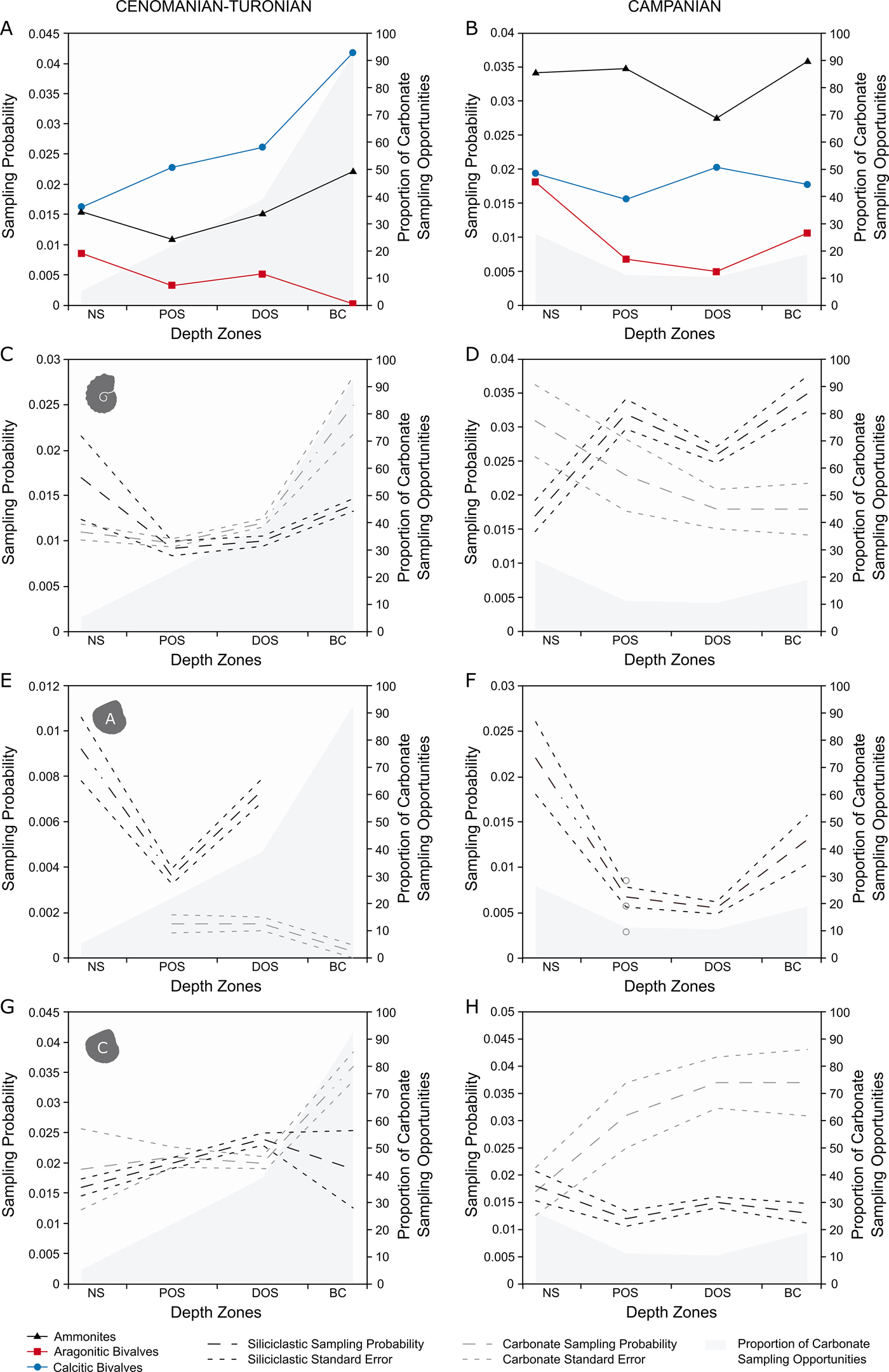
Figure 4. Plots of generic-level M2 sampling probabilities for the Cenomanian–Turonian (A, C, E, G) and lower Campanian (B, D, F, H) time slices across depth zones, split into carbonate and siliciclastic sampling opportunities. All results are plotted with percentage of carbonate collections per depth zone. A, Cenomanian–Turonian generic-level sampling probability, plotted with percentage of carbonate collections per depth zone; B, lower Campanian generic-level sampling probability, plotted with percentage of carbonate collections per depth zone; C, Cenomanian–Turonian ammonite sampling probability; D, lower Campanian ammonite sampling probability; E, Cenomanian–Turonian aragonitic bivalve sampling probability; F, lower Campanian aragonitic bivalve sampling probability; G, Cenomanian–Turonian calcitic bivalve sampling probability; H, lower Campanian calcitic bivalve sampling probability.
Campanian
In the lower Campanian (Fig. 4B), ammonites have the highest sampling probabilities, showing a level trend across the seaway with a pronounced trough in the distal offshore. Aragonitic bivalves record a relative high sampling probability in the nearshore, followed by a sharp decline for both proximal and distal offshore zones and an increase toward the basin center. Calcitic fauna have a consistently higher sampling probability than aragonitic bivalves, but lower than ammonites; they also show a level trend across the seaway, experiencing a peak in the distal offshore.
Sampling Probability between Lithologies
Cenomanian–Turonian
For the Cenomanian–Turonian (Fig. 4C,E,G), ammonites show the same trends and relatively little difference in absolute values between carbonate and siliciclastic sampling opportunities; the greatest difference appears in the basin center, where sampling probability is higher in carbonates. Aragonitic bivalves show a much larger difference, with siliciclastic opportunities scoring consistently higher than carbonate opportunities, even during the large decline within the proximal offshore. Calcitic bivalves show virtually no difference in sampling probability until the basin center, where sampling probability within carbonate sampling opportunities increases substantially.
Campanian
For the Campanian (Fig. 4D,F,H), siliciclastic opportunities of ammonites score higher than carbonate, except for within the nearshore. Aragonitic bivalves are not sampled within carbonate collections in either the nearshore, distal offshore, or basin center; their sampling probability curve is virtually entirely made by appearances in siliciclastic sampling opportunities. Calcitic bivalves show a decoupled trend between lithologies, with carbonate sampling opportunities showing higher on average sampling probabilities that increase toward the basin center, compared with the fairly low-scoring, level trend in siliciclastic.
Multiple Logistic Regression
Results of the logistic regressions are shown in Tables 1–8 and summarized in Figure 5. When interpreting these, note that calcitic mineralogy is compared with aragonitic mineralogy, so that positive regression coefficients indicate greater odds of sampling calcite. As lithology has multiple parameters, these were compared against the relative sampling probability of mudstone, which is used as a baseline. We are primarily interested in reporting effect sizes, which are gauged by the magnitude of regression coefficients.
Table 1. Table for multiple logistic regression results for all bivalves within the Cenomanian–Turonian across the whole seaway, using the model with lowest Akaike information criterion (AIC) score. M, mineralogy; D, diet; L, lithology; Z, depth zone; DOS, distal offshore; NS, nearshore; POS, proximal offshore. *indicates statistical significance at p = < 0.05.
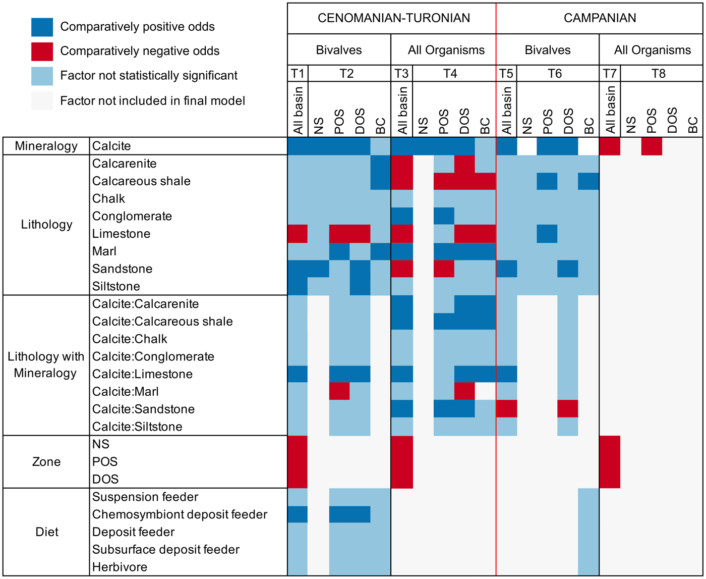
Figure 5. Graph summarizing multiple logistic regression model results (T1–T8 = Tables 1–8). Final models are presented within columns, whereas factors are presented along rows for those models. Results for factors are presented as either comparatively positive or negative odds of sampling compared with reference factor, not statistically significant, or not included in the final model. The following factors are used as a baseline for comparison: mineralogy, aragonite; lithology, mudstone; lithology with mineralogy, aragonite:mudstone; zone, basin center (BC); diet, carnivore. Note that the magnitude of regression coefficients is not presented within this graph. NS, nearshore; POS, proximal offshore; DOS, distal offshore.
AIC scores are utilized in choosing ideal model fit when comparing models with and without two-way interactive terms (a combination of effects between explanatory parameters: e.g., the relative odds of sampling calcitic fauna within a specific lithology), with lower scores indicating a better model fit. Only models with the lowest AIC scores are presented here, and we only report factors with statistically significant results (p < 0.05); full results can be found within Supplementary Information 2.
Cenomanian–Turonian
Mineralogy, lithology, feeding style, and depth zone all influence the preservation potential of fauna in the seaway (Table 1); lower AIC scores when an interactive term is added suggest this provides a better model fit than when it is excluded. The odds of sampling calcitic fauna are shown to be 4.6 times (the exponential of the coefficient; 1.52) higher that of aragonitic fauna, with analysis of variance (ANOVA) results showing mineralogy contributing the most toward deviance from the null model. Limestone environments are shown to be detrimental to the sampling probability of fauna, whereas sandstones and siltstone enhance sampling probability. The positive interaction between mineralogy and limestone lithologies shows that aragonitic fauna have comparatively strongly reduced odds of being sampled within limestone environments. All depth zones are shown to have decreased sampling probability compared with the basin center, with nearshore and proximal offshore zones showing the worst sampling potential. Chemosymbiont deposit feeders are shown to have an increased preservation potential compared with other feeding styles.
We additionally partitioned the data into each depth zone to test for differences with increased bathymetry across the seaway (Table 2). The nearshore zone exhibits an increase in the odds of sampling calcitic fauna, although this effect is reduced compared with results across the whole seaway. Sandstones are also shown to exhibit increased sampling probability. The proximal offshore shows a significant increase in the odds of sampling calcitic bivalves relative to aragonitic bivalves (6.17 compared with 1.88 for the nearshore), as well as increased sampling probability in marl depositional environments and for chemosymbiotic deposit feeders. Limestone negatively impacts the sampling probability of bivalves; the positive interaction between calcite and limestone consequently suggests that this negative impact is related to the sampling probability of aragonitic bivalves. The distal offshore shows a similar pattern, although the relative odds of each are reduced compared with the proximal offshore. The basin center shows increased odds of sampling bivalves within calcarenite, calcareous shale, and marl environments, but no other statistically significant terms.
Table 2. Table for multiple logistic regression results for all bivalves within the Cenomanian–Turonian for each depth zone, using the models with lowest Akaike information criterion (AIC) scores. M, mineralogy; D, diet; L, lithology. * indicates statistical significance at p = <0.05.
We also assessed depth zones for the inclusion of all organisms (Table 3). When ammonites are included, the odds of sampling aragonitic fauna increase (calcitic bivalves show odds of 2.1 higher sampling probability). Sandstone shows reduced odds of sampling any fauna, the opposite of previous results. The interaction between mineralogy and lithology shows increased sampling probability of calcitic organisms within limestones, sandstones, calcarenites, and calcareous mudstones, suggesting this effect is predominantly produced by the addition of ammonite fauna.
Table 3. Table for multiple logistic regression results for all organisms (including ammonites) within the Cenomanian–Turonian across the whole seaway, using the model with lowest Akaike information criterion (AIC) score. M, mineralogy; L, lithology; Z, depth zone; DOS, distal offshore; NS, nearshore; POS, proximal offshore. * indicates statistical significance at p = < 0.05.
When zones are assessed independently (Table 4), nearshore sampling probabilities are only controlled by mineralogy, although again with lower odds than reported elsewhere (1.56). In the proximal offshore, results show an increased sampling probability of calcitic fauna within sandstones and calcareous mudstones. The distal offshore also shows strong interactions between sampling probability of calcitic fauna and lithology, with strongly positive coefficients for sandstone, limestone, calcareous shale, and calcarenite two-way interactions. Overall, the sampling probability of calcite compared with aragonitic fauna is high, although reduced compared with the proximal offshore. Within the basin center, mineralogy is not listed as a statistically significant interactive term on its own, but calcitic fauna exhibit increased sampling probability for interactive terms with calcarenites, calcareous mudstones, limestones, and marls.
Table 4. Table for multiple logistic regression results for all organisms (including ammonites) within the Cenomanian–Turonian for each depth zone, using the models with lowest Akaike information criterion (AIC) scores. M, mineralogy; L, lithology. *indicates statistical significance at p = < 0.05.
Campanian
Models for all bivalves in the Campanian (Table 5) show comparatively few statistically significant contributors to sampling probability. By comparison with the Cenomanian, bivalve samples from the Campanian are only weakly influenced by mineralogy (showing odds of 2.16 increased likelihood of sampling calcitic organisms). Additionally, only sandstone and interactions between sandstone and limestone with calcitic organisms are shown to exert any other influence on sampling probability.
Table 5. Table for multiple logistic regression results for all bivalves within the lower Campanian across the whole seaway, using the model with lowest Akaike information criterion (AIC) score. M, mineralogy; D, diet; L, lithology; Z, depth zone. * indicates statistical significance at p = < 0.05.
This trend continues when partitioning the bivalve data into depth zones (Table 6). The nearshore zone has no statistically significant individual factors contributing to sampling probability. The proximal offshore includes statistically significant effects due to mineralogy and lithology, particularly limestones and calcareous mudstones, where sampling probability is enhanced. Mineralogy, sandstone, and the interaction between mineralogy and sandstone are reported as statistically significant factors for the distal offshore; mineralogy has a relatively high positive coefficient (odds of 3.16 in favor of calcitic organisms). Sampling probability is enhanced in sandstones overall, but negatively influences the odds of recovering calcitic organisms: it therefore follows that aragonitic bivalves show particularly enhanced sampling within sandstones. Model results for the basin center suggest that only calcareous shale has a statistically significant positive impact on sampling probability.
Table 6. Table for multiple logistic regression results for all bivalves within the lower Campanian for each depth zone, using models with lowest Akaike information criterion (AIC) scores. M, mineralogy; D, diet; L, lithology; Z, depth zone. *indicates statistical significance at p = < 0.05.

When all organisms are assessed (Table 7), mineralogy and depth zone are the only contributors to the full model. Surprisingly, aragonitic organisms have a higher sampling probability than calcitic organisms using the full model, with mineralogy only contributing to a very small amount of deviance from the null ANOVA model. As this result is not observed when assessing bivalve fauna, it is likely that ammonite occurrences are principally contributing to this effect.
Table 7. Table for multiple logistic regression results for all organisms (including ammonites) within the lower Campanian across the whole seaway, using model with lowest Akaike information criterion (AIC) score. M, mineralogy; L, lithology; Z, depth zone; DOS, distal offshore; NS, nearshore; POS, proximal offshore. * indicates statistical significance at p = < 0.05.

Depth zones were also evaluated for all organisms (Table 8). Only the proximal offshore supported a model other than the null, which reported mineralogy as a contributing factor; unusually, calcitic fauna are shown to have a reduced sampling probability compared with aragonitic fauna.
Table 8. Table for multiple logistic regression results for all organisms (including ammonites) within the lower Campanian for each depth zone, using models with lowest Akaike information criterion (AIC) scores. M, mineralogy; L, lithology; NULL, null model.
Range Size
Cenomanian–Turonian
Box plots were generated on a log scale to show differences in mean range sizes between calcitic and aragonitic organisms (Fig. 6A). There is a visible difference in variability of range size between groupings, with calcitic fauna showing an average larger range than aragonitic fauna. The Wilcoxon-Mann-Whitney test also showed a statistically significant difference between the range sizes for the two groups (p-value = 0.00405), with a reported difference in median range size of 48,694 km2. As sample size varied between the groups, resampling measures were carried out to test the accuracy of these results. A randomized bootstrap with replacement calculating the difference between the means of range sizes was implemented 10,000 times in R (Fig. 6C). Our recorded difference in the mean was shown to have an associated p-value of 0.0172, showing statistical significance.
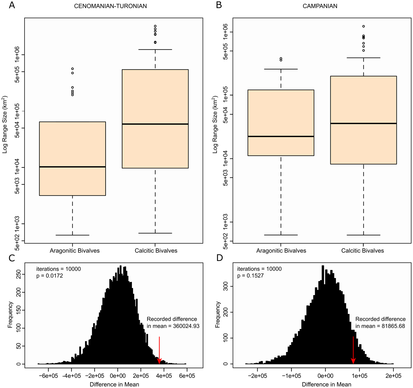
Figure 6. Range-size plots for the Cenomanian–Turonian and lower Campanian. A, Cenomanian–Turonian box plots of range size for both aragonitic bivalves and calcitic bivalves on log scale; B, lower Campanian box plots of range size for both aragonitic bivalves and calcitic bivalves on log scale; C, randomized bootstrap for Cenomanian–Turonian mean range sizes—recorded difference in the mean is shown to be statistically significant; D, randomized bootstrap for lower Campanian mean range sizes—recorded difference in the mean is not shown to be statistically significant.
Campanian
Box plots were generated to show differences in mean range sizes between early Campanian calcitic and aragonitic organisms (Fig. 6B). Calcitic bivalves show higher variability in mean range size than aragonitic bivalves. However, the Wilcoxon-Mann-Whitney test showed no statistically significant difference between the two groupings (p-value = 0.504) with a recorded difference in median range size of 13,540 km2, and a randomized bootstrap (Fig. 6D) with replacement recovered an associated p-value of 0.1527 (non-statistically significant).
Raw Diversity and SQS
Cenomanian–Turonian
Within the Cenomanian–Turonian, broadly similar patterns of diversity occur in all groups (Fig. 7A,C)—peak diversity is within the distal offshore, with lowest values in the nearshore and basin center. Calcitic bivalves show proportionally enhanced diversity in the proximal offshore compared with the other faunal groups. These patterns closely align with the number of collections within each zone, but show limited similarity to zoned outcrop area.
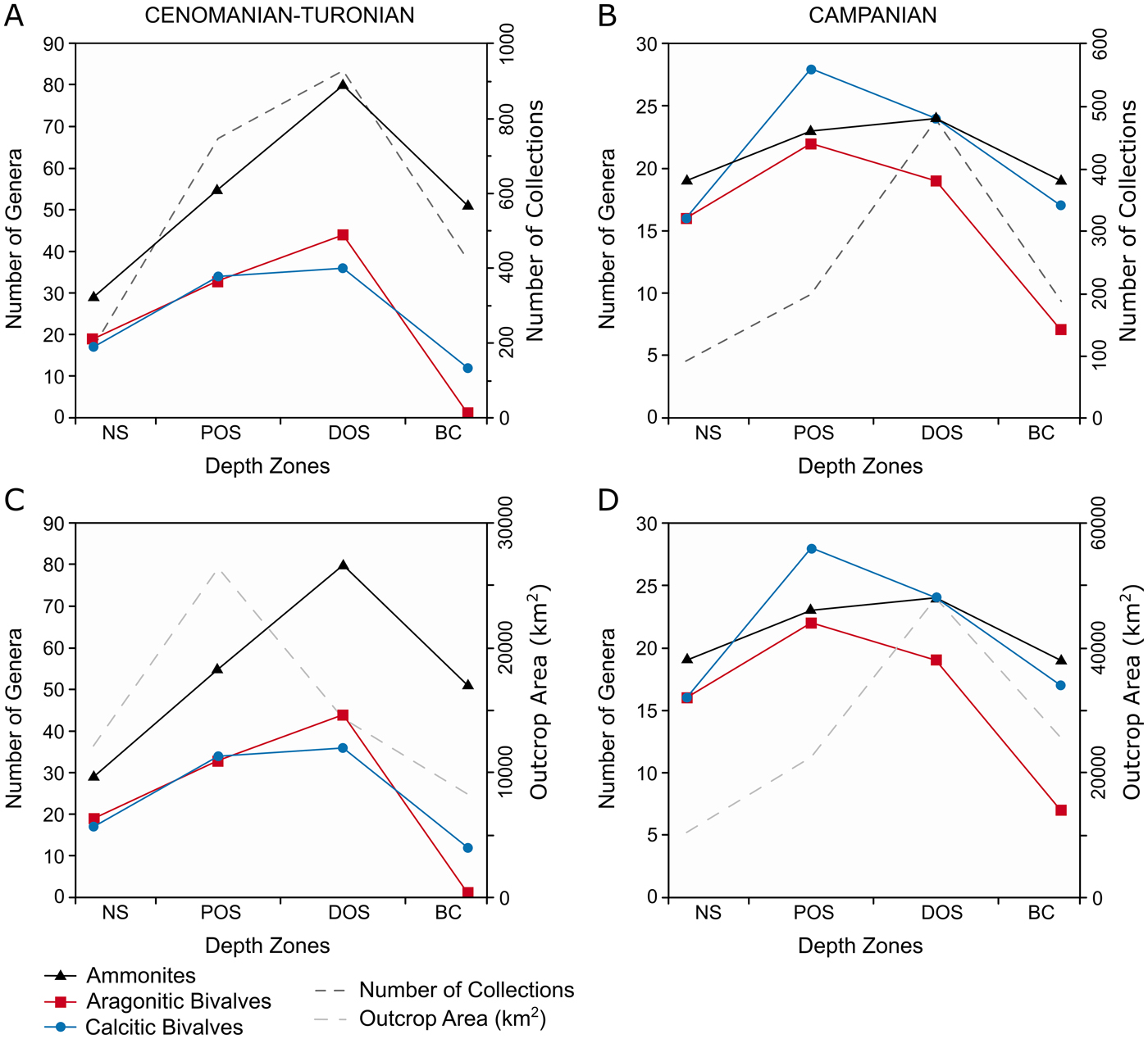
Figure 7. Plots of generic-level diversity plots for the Cenomanian–Turonian and lower Campanian within depth zones, plotted with number of collections and outcrop area. A, Generic diversity and number of collections for the Cenomanian–Turonian; B, generic diversity and number of collections for the lower Campanian; C, generic diversity and outcrop area for the Cenomanian–Turonian; D, generic diversity and outcrop area for the lower Campanian.
Subsampled ammonite and calcitic bivalve diversities show a broadly similar pattern to their raw taxic diversity signals (Fig. 8A,E). The record of aragonitic bivalves (Fig. 8C) is too poor to resolve subsampled diversity for the basin center; however, a slight decline in subsampled generic richness exists in the proximal offshore.
Figure 8. Plots of generic-level SQS results for depth zones in the Cenomanian–Turonian and lower Campanian, set at 0.4, 0.5, and 0.6 quora. A, SQS results for ammonites in the Cenomanian–Turonian; B, SQS results for ammonites in the lower Campanian; C, SQS results for aragonitic bivalves in the Cenomanian–Turonian; D, SQS results for aragonitic bivalves in the lower Campanian; E, SQS results for calcitic bivalves in the Cenomanian–Turonian; F, SQS results for calcitic bivalves in the lower Campanian.
Campanian
Calcitic bivalves and ammonites exhibit a similar pattern in diversity (Fig. 7B,D) although the latter show an increase in the proximal offshore. Aragonitic bivalve diversity has a similar peak in the proximal offshore but declines toward the basin center. None of these trends show similarity to the distribution of collections or outcrop area throughout the seaway.
When subsampled (Fig. 8B,D,F), calcitic and aragonitic bivalves are most diverse within the proximal offshore, falling to relative lows within the distal offshore and basin center. Ammonites are most diverse in the nearshore, followed by a decline to a flat profile.
Discussion
Sampling Probability and Multiple Logistic Regression
Our results from estimations of sampling probability and subsequent multiple logistic regression suggest that aragonite bias may be present within distinct depth zones of the seaway during the Cenomanian–Turonian. Mineralogy has a strong and statistically significant impact on sampling probability within the proximal and distal offshore bathymetric zones and shows the highest contribution to deviance from the null model. This is further supported by the fact that while all aragonitic taxa have lower sampling proportions overall, both aragonitic bivalves and ammonites disproportionally decrease in sampling probability within the proximal offshore compared with calcitic bivalves. Ammonites, while still showing reduced sampling probability compared with calcitic fauna, are more likely to be sampled than aragonitic bivalves; a potential explanation for this difference could be that aragonite dissolution acts differently upon ammonites compared with bivalves. Body sizes of ammonites and bivalves differ, with ammonites generally having larger forms (Jablonski Reference Jablonski, Jablonski, Erwin and Lipps1996). This has been known to influence preservation potential and the extent of aragonite dissolution: Wright et al. (Reference Wright, Cherns and Hodges2003) showed that ammonites are affected less severely than aragonitic bivalves by early-stage aragonite dissolution, often exhibiting poor preservation rather than complete removal. Our results have the potential to be partially related to this effect.
Aragonitic bivalves have lower absolute sampling probabilities in carbonate environments than in siliciclastic environments, supporting the results of Foote et al. (Reference Foote, Crampton, Beu and Nelson2015). However, when examining the proximal offshore zone, we can see that sampling probability within siliciclastic lithologies falls dramatically. As this zone records the largest difference in odds of sampling between calcitic and aragonitic taxa, it can be argued that aragonite bias can influence fauna within siliciclastic deposits in epicontinental seas, in contradiction to Foote et al. (Reference Foote, Crampton, Beu and Nelson2015). The absolute sampling proportions of calcitic bivalves remain relatively consistent (at ~2% of genera per collection) throughout the seaway until the basin center, where they increase dramatically within carbonates compared with siliciclastics. Foote et al. (Reference Foote, Crampton, Beu and Nelson2015) reported that calcitic organisms experienced higher sampling probabilities in carbonate-rich intervals, which is especially enhanced in limestones. As carbonates make up ~93% of total sampling opportunities within this zone, our results align fairly closely with previous findings. While Foote et al. (Reference Foote, Crampton, Beu and Nelson2015) singled out lithology as an important factor for aragonite dissolution, they did not investigate whether differences in grain size significantly influenced results. Within this study, sandstone and siltstone are consistently shown to have better odds at preserving aragonitic fauna than mudstone. This is unsurprising, considering that coarser, oxidized sediments are likely to contain lower quantities of organic matter than finer sediments, and thus provide less material for the microbial decay that ultimately controls the dissolution of aragonite within the TAZ (Cherns et al. Reference Cherns, Wheeley and Wright2008). However, siltstone appears to have higher odds than sandstone, potentially a reflection of increased quality of preservation in lower-energy settings. It should be noted, however, that only a few models include both siltstone and sandstone and therefore allow for comparison of sampling probabilities of these two lithologies.
Potential ecological signals can also be parsed from the results reported here. Within the Cenomanian–Turonian data set, odds of sampling chemosymbiont deposit feeders within the proximal offshore were higher than for sampling other bivalves, forming a statistically significant part of the final model and accounting for the second highest deviance from the null model. Chemosymbiosis in bivalves occurs in a range of environments to cope with life in sulfide-rich environments, typically at deep sea vents or in sediments at the oxic/anoxic interface (Cavanaugh Reference Cavanaugh1994). Combined with evidence for poor sampling probability of aragonitic fauna in siliciclastic lithologies, this lends credence to the likelihood of fluctuating benthic oxygen conditions within the proximal offshore, ideal for preferential aragonite dissolution. More broadly, several previous works have suggested that aragonite bias strongly influences perceived trophic communities within molluscan fauna, favoring preservation of specific life habits (Cherns et al. Reference Cherns, Wheeley and Wright2008; Cherns and Wright Reference Cherns and Wright2009). Unfortunately, very few statistically significant life habit factors contribute to our final models (Fig. 5), and thus we cannot draw any conclusions regarding preservational shifts in trophic structure. In the basin center, ammonites are more likely to be sampled compared with other organisms. This confirms expectations of enhanced preservation within a predominantly anoxic water column, where dissolution and predation have reduced impact on the removal of fauna emplaced by pelagic fallout (Jordan et al. Reference Jordan, Allison, Hill and Sutton2015).
Within the Campanian, there is a somewhat contradictory pattern. Multiple logistic regression results show that mineralogy only has a strong, statistically significant impact on relative sampling odds when assessing bivalves within the proximal and distal offshore bathymetric zones, with only the latter showing a strong deviation from the null model in ANOVA results. When ammonites are added, the odds of sampling aragonitic fauna are actually higher than for calcitic organisms within the proximal offshore, and all other zones show no statistically significant contributions from mineralogy. This is reinforced when one considers the absolute proportions of mineralogies sampled: ammonites exhibit the highest overall sampling probability among fauna. A potential cause of this contradiction is preferential sampling bias. Ease of collecting and human interest can result in skewed sampling effort and intensity, potentially inflating (Foote and Sepkoski Reference Foote and Sepkoski1999) or reducing (Lloyd and Friedman Reference Lloyd and Friedman2013) the published records of certain taxa, locations, and time periods above others. The WIS has long been known for its abundance and diversity of ammonite fauna, and consequently ammonites have been used for systematic biostratigraphic correlation since the 1930s (Stephenson and Reeside Reference Stephenson and Reeside1938). An intensive effort to collect ammonites for stratigraphic purposes was carried out by a selection of workers through the latter half of the twentieth century to the present day (Scott and Cobban Reference Scott and Cobban1959; Gill and Cobban Reference Gill and Cobban1973; Cobban and Hook Reference Cobban, Hook and Westerman1984; Cobban et al. Reference Cobban, Walaszczyk, Obradovich and McKinney2006; Merewether et al. Reference Merewether, Cobban and Obradovich2011). Consequently, it is likely that records for biostratigraphically important organisms have been overinflated compared with other mollusks and between localities. By comparing previously existing collections and newly collected records for the upper Cenomanian Sciponoceras gracile Zone (now the Vascoceras diartianum Zone and the Euomphaloceras septemseriatum Zone; Cobban et al. Reference Cobban, Walaszczyk, Obradovich and McKinney2006), Koch (Reference Koch1978) showed that ammonites were better studied and more commonly reported than bivalve fauna. Parts of these collections have made up the majority of the publicly available records of fossil occurrences within the WIS that are used in this study. As such, it is possible that ammonites are overrepresented in the early Campanian data set and are skewing perceived results. However, it is still possible to suggest that a suppressed expression of spatial aragonite bias occurs in the distal offshore, albeit at reduced levels in comparison to the Cenomanian–Turonian interval.
Range Size
Range-size results reported a difference between calcitic and aragonitic bivalves across the two time intervals studied, with aragonitic fauna showing a significantly smaller range size during the Cenomanian–Turonian but not the Campanian. This variation is also expressed spatially (Fig. 9). Within the Cenomanian–Turonian time slice, aragonitic geographic ranges (Fig. 9A) are generally restricted to the western and northern edges of the seaway in comparison to calcitic geographic ranges, which extend farther to the center of the basin, as well as to the east and south (Fig. 9C). This same pattern is slightly different in the early Campanian interval (Fig. 9B,D); while aragonitic fauna still show a limited range, the difference between both bivalve groups is less pronounced. This pattern also matches with the distribution of carbonate deposition within the WIS: the Cenomanian–Turonian interval experienced widespread carbonate sedimentation—in the form of the Greenhorn Limestone Formation—in the basin center (Miall et al. Reference Miall, Catuneanu, Vakarelov, Post and Miall2008), while deposition in the basin center transitioned from limestones of the Niobrara Formation to the siliciclastic mudstones of the Pierre Shale in the early Campanian (McGookey et al. Reference McGookey, Haun, Hale, Goodell, McCubbin, Weimer and Wulf1972; Da Gama et al. Reference Da Gama, Lutz, Desjardins, Thompson, Prince and Espejo2014). As our results confirm that carbonate environments can exacerbate the effects of aragonite dissolution, it is possible that the differences between the Cenomanian–Turonian and the Campanian are partially driven by the enhanced effects of aragonite bias in carbonate-rich environments, resulting in a lowered sampling probability within carbonate-dominated localities.
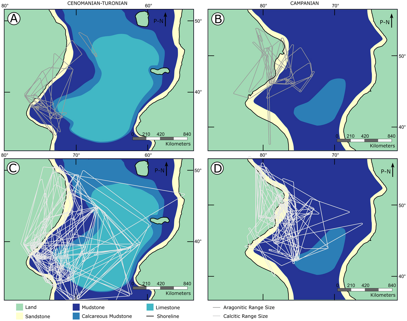
Figure 9. Paleogeographic maps shown with range sizes of calcitic and aragonitic bivalves for both time slices. A, Aragonitic bivalve range sizes for the Cenomanian–Turonian; B, aragonitic bivalve range sizes for the lower Campanian; C, calcitic bivalve range sizes for the Cenomanian–Turonian; D, calcitic bivalve range sizes for the lower Campanian. P-N indicates direction of paleo-north.
Occurrence and Diversity Results
Overall, there is some evidence of aragonite dissolution influencing patterns of pure occurrences and taxonomic and subsampled diversity for aragonitic fauna, as previously hypothesized. In the Cenomanian–Turonian, aragonite bias is most pronounced within the proximal offshore bathymetric zone, with a lesser impact within the distal offshore zone. While all fauna show a close correlation to collection counts for depth zones, both aragonitic and calcitic fauna deviate from this correlation in the proximal offshore zone, recording lower raw occurrences and diversity. The same is broadly observed in the Campanian: maximum disparity of sampling probability between calcitic and aragonitic fauna is observed within the distal offshore zone, where aragonitic occurrences and raw taxic diversity show a noticeable decline and subsequent deviation from sampling proxies. Foote et al. (Reference Foote, Crampton, Beu and Nelson2015) reported similar results when comparing sampling-corrected results to ones that previously displayed the proportion of aragonitic taxa (Crampton et al. Reference Crampton, Foote, Beu, Maxwell, Cooper, Matcham, Marshall and Jones2006) and concluded that similarities existed between sampling probabilities and relative proportions of aragonitic species.
Despite the potential relationships discussed earlier, we cannot report conclusive evidence for aragonite bias influencing the sampled diversity of molluscan fauna within the WIS. This aligns with other recent studies showing that despite evidence of widespread aragonite dissolution during early shallow diagenesis, perceived diversity is not largely affected by these processes (Behrensmeyer et al. Reference Behrensmeyer, Fürsich, Gastaldo, Kidwell, Kosnik, Kowalewski, Plotnick, Rogers and Alroy2005; Kidwell Reference Kidwell2005; Crampton et al. Reference Crampton, Foote, Beu, Maxwell, Cooper, Matcham, Marshall and Jones2006; Hsieh et al. Reference Hsieh, Bush and Bennington2019). Hence, we must additionally look at external influences that might capture, enhance, or control the distribution of aragonitic faunas that would otherwise be lost to preferential dissolution.
Known human influences have potentially contributed to the suppression of aragonite bias on a spatial scale. While the extent to which aragonite dissolution may have influenced our perceived record of molluscan diversity within the WIS is unclear, it is apparent that these records closely correlate with established sampling proxies. Results of Spearman rank correlation tests of occurrences and raw taxic diversity against sampling proxies for distance from paleoshoreline zones (Table 9) correlate strongly and significantly. It is clear that broader-scale sampling trends related to collector effort strongly influence the pattern of faunal distribution across the seaway, potentially overwriting the effects of aragonite dissolution.
Table 9. Spearman's rank correlations between generic diversity of faunal groups and various sampling proxies for distance from paleoshoreline zones within the Cenomanian–Turonian and lower Campanian. Sig., significance; * indicates statistical significance at p = < 0.05.
While there have been many cases of preferential aragonite dissolution within local studies, aragonitic molluscan fauna are relatively well represented in the global fossil record (Harper Reference Harper, Donovan and Paul1998). This paradox suggests that processes must occur that capture records of molluscan fauna at a higher frequency than the frequency at which they are capable of being destroyed. Cherns et al. (Reference Cherns, Wheeley and Wright2008, Reference Cherns, Wheeley and Wright2011) describe “taphonomic windows” as events in the fossil record that capture an unbiased view of aragonitic faunas that have escaped preferential dissolution, and these authors detail many examples that may have operated within the WIS. One such window that is prevalent within the WIS is concretions, sedimentary mineral masses of varying chemical composition that often form at shallow burial depths early in diagenesis when mineral cement precipitates locally during lithification (Berner Reference Berner1968; McCoy et al. Reference McCoy, Young and Briggs2015). These have the potential to preserve three-dimensional fossilized remains, often in exquisite detail (Dean et al. Reference Dean, Sutton, Siveter and Siveter2015; Korn and Pagnac Reference Korn and Pagnac2017). Concretions are also a characteristic mode of molluscan occurrences within the WIS, with fossil-bearing concretions found commonly throughout the seaway (Landman and Klofak Reference Landman and Klofak2012); as such, they could further contribute to a potential anthropogenic bias in that they provide easily spotted locations to find fauna in otherwise barren strata (such as the Pierre Shale), skewing collection intensity between localities with concretions and those without. However, only ~3% of USGS collections were obtained by selective collecting (Koch Reference Koch1980), and as USGS records make up ~55% of our finished data set, this suggests that sampling intensity bias might be partially mitigated. Sediment accumulation rate could exert a large influence on the potential for preferential aragonite dissolution to affect spatial zones of the seafloor. If sediment accumulation rates were low, fauna would remain within the TAZ for an extended period of time, and thus are more likely to be removed through physical reworking, bioerosion, and enhanced dissolution (Cherns et al. Reference Cherns, Wheeley and Wright2011). In contrast, if sediment accumulation rates were high, fauna are likely to have been rapidly buried and thus have escaped into the sub-TAZ region, where vulnerable bioclasts are likely to be stabilized by shallow-burial diagenesis (Melim et al. Reference Melim, Westphal, Swart, Eberli and Munnecke2002, Reference Melim, Swart and Eberli2004). Sediment accumulation rates within the WIS varied both longitudinally within a stratigraphic interval (with higher sediment accumulation rates toward the western paleoshoreline) and with increased bathymetry in a single location (Arthur and Sageman Reference Arthur, Sageman and Harris2005): accounting for this potential influence is problematic, and the extent of its effects is ambiguous. The result of these factors is a potential suppression of the spatial influence of aragonite dissolution bias on recorded faunal diversity within the WIS.
Spatial Scale and Influence of Bias
The issue of scale is key to understanding the spatial impact of aragonite dissolution (Kosnik et al. Reference Kosnik, Alroy, Behrensmeyer, Fürsich, Gastaldo, Kidwell, Kowalewski, Plotnick, Rogers and Wagner2011). Foote et al. (Reference Foote, Crampton, Beu and Nelson2015) recorded preferential aragonite bias within carbonate-rich environments on the regional spatial (~106 km2) and stage-level temporal (1–10 Myr) scales. However, others (Behrensmeyer et al. Reference Behrensmeyer, Fürsich, Gastaldo, Kidwell, Kosnik, Kowalewski, Plotnick, Rogers and Alroy2005; Kidwell Reference Kidwell2005; Kiessling et al. Reference Kiessling, Aberhan and Villier2008; Kosnik et al. Reference Kosnik, Alroy, Behrensmeyer, Fürsich, Gastaldo, Kidwell, Kowalewski, Plotnick, Rogers and Wagner2011) using global-scale data have reported negligible influence of shell mineralogy on temporal trends or frequency of occurrences. Foote et al. (Reference Foote, Crampton, Beu and Nelson2015) reported three key differences between previous studies and their work: higher taxonomic level of occurrences, larger time bins, and the use of global data. These factors were inferred to “even out” spatial and temporal variations in sampling, mitigating the influence and effect of locally variable biases inherent to the fossil record. Foote et al. (Reference Foote, Crampton, Beu and Nelson2015) further suggested that as their taxonomic and temporal scales were consistent with previously published work, an increase in spatial scale may prove the most influential factor in demoting the influence of aragonite dissolution.
This result can be easily translated into the spatial expression of aragonite bias by comparing its potential on alpha (within-site), beta (between-site), and gamma (global) diversity. At the alpha level, the impact of aragonite bias on a single species will be at its most severe, particularly within single-bed assemblages (Wright et al. Reference Wright, Cherns and Hodges2003; Bush and Bambach Reference Bush and Bambach2004; Cherns et al. Reference Cherns, Wheeley and Wright2008, Reference Cherns, Wheeley and Wright2011). However, at gamma levels of diversity, the probability of not recording an individual drops substantially due to the number of possible localities to sample from, where various taphonomic windows may result in aragonite preservation. As such, an increased number of localities in a spatial setting are likely to partially obscure localized aragonite dissolution. As we recorded an impact on zoned sampling probabilities and range size of aragonitic fauna in the WIS, but could not conclusively prove an influence on total diversity estimates, our data support the suggestions of Foote et al. (Reference Foote, Crampton, Beu and Nelson2015) that spatial scale is a dominant factor on the severity of aragonite bias.
While preferential aragonite dissolution is unlikely to influence diversity on a global scale, this study has shown that it has the capacity to govern the sampling probability of a species in geographic space, and thus can influence the “variation” definition of beta diversity (Anderson et al. Reference Anderson, Crist, Chase, Vellend, Inouye, Freestone, Sanders, Cornell, Comita and Davies2011). As the preferential dissolution of aragonite is a process that is exacerbated by certain environments (Foote et al. Reference Foote, Crampton, Beu and Nelson2015), its influence will impact localities with different environmental conditions to differing extents—a species will be lost at one site and recorded at another. Our results confirm this, showing aragonite bias has an effect on observed diversity between locations, at least during times of widespread carbonate deposition.
Consequently, when looking at the spatial signal of aragonite dissolution as a whole, we can see a sliding scale of influence: strong, environmentally dependent impact on alpha diversity; a potentially large influence on beta diversity; and a negligible impact on gamma diversity. Bush et al. (Reference Bush, Markey and Marshall2004) grouped biases affecting spatially organized biodiversity in similar alpha, beta, and gamma levels, with alpha biases influencing within-site diversity and beta and gamma arising from failure to sample all available habitats or environments within a region. While it was noted in this study that taphonomic effects were not included in this definition, this system can be modified in the light of our results. Aragonite bias, while operating at an alpha bias (local) level, evidently has the capacity to systematically influence estimates of beta diversity. As such, the influence of some taphonomic biases may be dependent on the spatial scale at which they are observed. This is an important consideration for studies of the spatial distribution of bias in the fossil record (Barnosky et al. Reference Barnosky, Carrasco and Davis2005; Vilhena and Smith Reference Vilhena and Smith2013; Benson et al. Reference Benson, Butler, Alroy, Mannion, Carrano and Lloyd2016; Close et al. Reference Close, Benson, Upchurch and Butler2017), and for paleobiogeographic studies in general.
Conclusions
1. A multifaceted approach shows that preferential aragonite dissolution is spatially variable and impacts the relative likelihood, absolute sampling probabilities, and range sizes of aragonitic organisms within the Cretaceous WIS of North America for a time interval that straddles the Cenomanian/Turonian boundary. A similar but reduced effect is additionally observed within an early Campanian time interval. A combination of depositional lithology (a limestone-dominated basin within the Cenomanian–Turonian compared with a more siliciclastic setting in the early Campanian) and an anoxic basin center are hypothesized as drivers for this effect.
2. Carbonate environments enhance the effects of aragonite dissolution and the preservation of calcitic organisms, as has been previously demonstrated. However, in contrast to previous studies, siliciclastic environments are also shown to be influenced by preferential aragonite dissolution.
3. While similarities are observed between faunal distribution and absolute sampling probabilities, we cannot conclusively say that aragonite dissolution has influenced perceived diversity of mollusks within the WIS. Taphonomic windows act to preserve records of organisms that would otherwise be lost. Other anthropogenic and geologic biases appear to have a more obvious effect on the molluscan record, and likely mask the influence of aragonite dissolution.
4. While aragonite bias can be thought of as an alpha bias, results show it could have a systematic and severe impact on beta diversity. This suggests that taphonomic biases can act differently at different scales in the spatial realm.
Acknowledgments
We would like to thank A. Quallington and Getech Group PLC for permission to use and edit the paleogeographic reconstructions in this study. We are especially thankful to S. Kidwell for providing molluscan mineralogy information, J. Alroy for providing the SQS function in R, and C. McKinney and K. Hollis for providing valuable museum data sets. We thank W. Kiessling, A. Bush, and one anonymous reviewer for comments that improved an earlier version of this work. We would also like to thank P. Wright, M. Sephton, S. Maidment, and A. Chiarenza for fruitful discussions regarding the article, as well as contributors to PhyloPic.org and the PBDB. C.D.D. was supported by a National Environmental Research Council (UK) studentship (1394514). This is Paleobiology Database official publication number 347.


 Open access