


1. Introduction
Finite-state time-homogenous Markov processes (chains) have been widely used in many areas, for example, in ion channel modeling [Reference Ball3, Reference Ball and Sansom5, Reference Colquhoun and Hawkes10] and in reliability modeling [Reference Ay, Soyer, Landon and Ozekici2, Reference Bao and Cui6–Reference Chiquet and Limnios8, Reference Cui and Kang15, Reference Eryilmaz16, Reference Finkelstein18, Reference Jianu, Ciuiu, Daus and Jianu20, Reference Wu, Cui and Fang26]. The evolution process of a finite-state time-homogenous Markov process is not always observed completely; sometimes, it can only be obtained partially, which depends on the operational situation and apparatus used. For the complete information evolution of the processes, there are lots of literature in both theory and practice. The situation of partially observable information on the evolution becomes more difficult, but there has been much literature at present since this case can be encountered in more practical circumstances. The aggregated stochastic processes can be used to decribe evolution processes with group information observed, for example, the underlying process is known to be in a subset of states instead of a specific state. In general, people name the aggregated stochastic process in terms of its underlying stochastic process. For example, if the underlying process possesses the Markov property, then the corresponding aggregated stochastic process is called an aggregated Markov stochastic process. The aggregated Markov and semi-Markov stochastic processes have been extensively used in ion channel modeling and reliability, for example, see Colquhoun and Hawkes [Reference Colquhoun and Hawkes11], Ball and Sansom [Reference Ball and Sansom4], Rubino and Sericola [Reference Rubino and Sericola24], Hawkes et al. [Reference Hawkes, Cui, Du, Frenkel, Karagrigoriou, Lisnianski and Kleyner19], Zheng et al. [Reference Zheng, Cui and Hawkes31], Cui et al. [Reference Cui, Du and Hawkes12–Reference Cui, Du and Zhang14], and Yi et al. [Reference Yi, Cui and Balakrishnan27–Reference Yi, Cui, Balakrishnan and Shen29]. Of course, there are some differences on the studies of aggregated stochastic processes in ion channel modeling and reliability. For example, the assumptions on the underlying processes and research contents have some differences. In ion channel modeling, the underlying Markov processes are assumed to possess time reversibility, which is not needed in reliability. In research contents, the steady-state behaviors are considered in both subjects, but in reliability, studying the instantaneous properties of the aggregated stochastic processes is one of the important tasks under the given initial state.
As mentioned above, in reliability, the limiting behaviors have been studied already, which are mainly done by obtaining the instantaneous measures when time t approaches infinity [Reference Angus1]. It is well known that the limiting behaviors of the underlying Markov process do not depend on the initial state in most cases in terms of the common knowledge of Markov processes [Reference Pollett and Taylor23, Reference Wang, Wu and Zhu25]. Thus, the corresponding aggregated Markov process also has this property [Reference Katehakis and Smit21]. However, based on the corresponding formulas derived from the aggregated Markov processes, it is difficult to get this conclusion directly. In detail, the steady-state measures are obtained in aggregated Markov processes using the Laplace transforms. In terms of Tauber’s theorem, the steady-state measures equal to the limits of the products of an s and the Laplace transforms of steady-state measures when s approaches zero from the right side. The Laplace transforms of steady-state measures contain the initial state probabilities, which, in general, are matrices or vectors. Thus, unlike one-dimensional case, it is hard to see that the initial state probabilities do not play any role in the steady-state measures. More details are given in Section 3. The aims of this paper are to present the rigorous proof on this conclusion, that is the four steady-state measures given in the paper do not depend on the initial state. The detailed contributions of the paper include the following: (i) Under the condition  ${\rm{Rank}}({\bf{Q}}) = n - 1$ (the dimension of matrix Q is n × n), which includes the case that all states communicate each other, the proof that four steady-state measures expressed by Laplace transforms do not depend on the initial state is presented; (ii) A numerical example on the condition ${\rm{Rank}}({\bf{Q}}) = n - 2$ is discussed and the rank of the transition rate matrix also is studied; and (iii) This proof can bridge a gap between the common knowledge in Markov processes and aggregated Markov processes for the case of steady-state situation.
The organization of the paper is as follows. In Section 2, some basic knowledge on the aggregated Markov processes and the inversion on four-block paritioned matrix are presented. Meanwhile, the proof for that  ${\rm{Rank}}({\bf{Q}}) = n - 1$ for the case that all states communicate with each other is given. The four steady-state measures expressed by Laplace transforms are derived, and two essential terms are abstracted for the later contents in the paper in Section 3. In Section 4, the main results that two essential terms that contain the four steady-state measures do not depend on the initial state are presented. Three different numerical examples are given to illustrate the direct ways for the limiting results in Section 5; especially, some discussions are presented, which may be useful for the case of ${\rm{Rank}}({\bf{Q}}) \le n - 2$. Finally, the paper is concluded in Section 6.
Throughout this paper, vectors and matrixes are rendered in bold, namely, u denotes a column vector of ones, I denotes an identity matrix, and 0 denotes a matrix (vector) of zeros, whose dimensions are apparent from the context. Besides, the symbol T denotes a transpose operator as a superscript.
2. Preliminaries
In this section, some basic knowledge on the theory of aggregated Markov process are presented, which are developed in pathbreaking papers such as Colquhoun and Hawkes [Reference Colquhoun and Hawkes11] in the ion channel literature and other papers like Ball and Sansom [Reference Ball and Sansom5] in the probability literature and Rubino and Sericola [Reference Rubino and Sericola24] and Zheng et al. [Reference Zheng, Cui and Hawkes31] in the reliability literature. These knowledge form our basic concepts and notations in this paper. The basic assumptions to be used are also discussed, and the proofs of some of them are given in this section.
Consider a finite-state homogenous continuous-time Markov process  $\{X(t),t \ge 0\}$ with transition rate matrix ${\bf{Q}} = {\left( {{q_{ij}}} \right)_{n \times n}}$, state space ${\bf{S}} = \{1,2, \ldots ,n\} $, and initial probability vector ${{\bf{\alpha }}_0} = ({\alpha _1},{\alpha _2}, \ldots ,{\alpha _n})$. The stochastic process $\{X(t),t \ge 0\}$ can result from many areas such as ion channel, quality and reliability, operational management, and so on. With many possible reasons, the state space can be assumed to be aggregated by partitioning into classes, so that it is possible to observe only which class the stochastic process is in at any given time instead the specific state it is in. This fact forms a new stochastic process $\{\tilde X(t),t \ge 0\} $ with state space ${\tilde{\bf{S}}}$ such that $|{\tilde{\bf{S}}}| \lt |{\bf{S}}|$, that is, each class in S is a state in ${\tilde{\bf{S}}}$. The stochastic process $\{\tilde X(t),t \ge 0\} $ is called an aggregated Markov process, and the stochastic process $\{X(t),t \ge 0\} $ is called the underlying one. In reliability field, in general, the state space S can be divided into two classes: the working (up) class, denoted by W, and the failure (down) class, denoted by F, that is, ${\bf{S}} = {\bf{W}} \cup {\bf{F}}$. Without loss of generality, it is assumed that ${\bf{W}} = \{1,2, \ldots ,{n_o}\}$ and ${\bf{F}} = \{{n_o} + 1,{n_o} + 2, \ldots ,n\}$. The corresponding transition rate matrix Q can also be written as
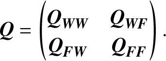 \begin{equation}
{\bf{Q}} = \left( {
\begin{matrix}
{{{\bf{Q}}_{{\bf{WW}}}}} & {{{\bf{Q}}_{{\bf{WF}}}}} \\
{{{\bf{Q}}_{{\bf{FW}}}}} & {{{\bf{Q}}_{{\bf{FF}}}}}
\end{matrix}
} \right).
\end{equation}
\begin{equation}
{\bf{Q}} = \left( {
\begin{matrix}
{{{\bf{Q}}_{{\bf{WW}}}}} & {{{\bf{Q}}_{{\bf{WF}}}}} \\
{{{\bf{Q}}_{{\bf{FW}}}}} & {{{\bf{Q}}_{{\bf{FF}}}}}
\end{matrix}
} \right).
\end{equation}To study the aggregated Markov process, the following concepts and notation are given:
 \begin{align}
{}^{\bf{W}}{p_{ij}}(t): = P\{& X(t){\rm{~remains~within~}}{\bf{W}}{\rm{~throughout~time~0~to~time~}}t, \nonumber\\
& {\rm{and~is~in~state~}}j{\rm{~at~time~}}t|X(0) = i\}, \quad{\rm}i,j \in {\bf{W}}.
\end{align}
\begin{align}
{}^{\bf{W}}{p_{ij}}(t): = P\{& X(t){\rm{~remains~within~}}{\bf{W}}{\rm{~throughout~time~0~to~time~}}t, \nonumber\\
& {\rm{and~is~in~state~}}j{\rm{~at~time~}}t|X(0) = i\}, \quad{\rm}i,j \in {\bf{W}}.
\end{align} After simple manipulations, we get, in matrix form,  ${}^{\bf{W}}{p_{ij}}(t)$ are the elements of the ${n_o} \times {n_o}$ matrix
 \begin{equation}
{{\bf{P}}_{{\bf{WW}}}}(t) = {\left( {{}^{\bf{W}}{p_{ij}}(t)} \right)_{{n_o} \times {n_o}}} = \exp ({{\bf{Q}}_{{\bf{WW}}}}t).
\end{equation}
\begin{equation}
{{\bf{P}}_{{\bf{WW}}}}(t) = {\left( {{}^{\bf{W}}{p_{ij}}(t)} \right)_{{n_o} \times {n_o}}} = \exp ({{\bf{Q}}_{{\bf{WW}}}}t).
\end{equation}Another important quantity is defined as
 \begin{align}
{g_{ij}}(t): = \mathop {\lim }\limits_{\Delta t \to 0} [P\{& X(t){\rm{~stays~in~}}{\bf{W}}{\rm{~from~time~0~to~time~}}t,{\rm{~and~leaves~}}{\bf{W}}{\rm{~for~state~}}j \nonumber\\
& {\rm{~between~}}t{\rm{~and~}}t + \Delta t|X(0) = i\} /\Delta t], \quad{\rm}i \in {\bf{W}},j \in {\bf{F}}.
\end{align}
\begin{align}
{g_{ij}}(t): = \mathop {\lim }\limits_{\Delta t \to 0} [P\{& X(t){\rm{~stays~in~}}{\bf{W}}{\rm{~from~time~0~to~time~}}t,{\rm{~and~leaves~}}{\bf{W}}{\rm{~for~state~}}j \nonumber\\
& {\rm{~between~}}t{\rm{~and~}}t + \Delta t|X(0) = i\} /\Delta t], \quad{\rm}i \in {\bf{W}},j \in {\bf{F}}.
\end{align} Similarly, we have, in matrix form,  ${g_{ij}}(t)$ are the elements of the ${n_o} \times (n - {n_o})$ matrix
 \begin{equation}
{{\bf{G}}_{{\bf{WF}}}}(t) = {{\bf{P}}_{{\bf{WW}}}}(t){{\bf{Q}}_{{\bf{WF}}}}.
\end{equation}
\begin{equation}
{{\bf{G}}_{{\bf{WF}}}}(t) = {{\bf{P}}_{{\bf{WW}}}}(t){{\bf{Q}}_{{\bf{WF}}}}.
\end{equation} The Laplace transform will be used throughout the paper, which is defined for function f(t) as  ${f^*}(s) = \int_0^\infty {{{\rm e}^{- st}}f(t)\,{\rm{d}}t}$. The Laplace transform for a functional matrix is defined elementwise. The Laplace transforms of Eqs. (2.3) and (2.5), respectively, are
 \begin{align}
{\bf{P}}_{{\bf{WW}}}^*(s) = {(s{\bf{I}} - {{\bf{Q}}_{{\bf{WW}}}})^{- 1}},
\end{align}
\begin{align}
{\bf{P}}_{{\bf{WW}}}^*(s) = {(s{\bf{I}} - {{\bf{Q}}_{{\bf{WW}}}})^{- 1}},
\end{align} \begin{align}
{\bf{G}}_{{\bf{WF}}}^*(s) = {\bf{P}}_{{\bf{WW}}}^*(s){{\bf{Q}}_{{\bf{WF}}}} = {(s{\bf{I}} - {{\bf{Q}}_{{\bf{WW}}}})^{- 1}}{{\bf{Q}}_{{\bf{WF}}}},
\end{align}
\begin{align}
{\bf{G}}_{{\bf{WF}}}^*(s) = {\bf{P}}_{{\bf{WW}}}^*(s){{\bf{Q}}_{{\bf{WF}}}} = {(s{\bf{I}} - {{\bf{Q}}_{{\bf{WW}}}})^{- 1}}{{\bf{Q}}_{{\bf{WF}}}},
\end{align} ${\bf{G}}_{{\bf{WF}}}^*(0)$ will be briefly denoted as ${{\bf{G}}_{{\bf{WF}}}}$, that is,
 \begin{equation}
{{\bf{G}}_{{\bf{WF}}}} = {\bf{G}}_{{\bf{WF}}}^*(0) = - {\bf{Q}}_{{\bf{WW}}}^{- 1}{{\bf{Q}}_{{\bf{WF}}}}.
\end{equation}
\begin{equation}
{{\bf{G}}_{{\bf{WF}}}} = {\bf{G}}_{{\bf{WF}}}^*(0) = - {\bf{Q}}_{{\bf{WW}}}^{- 1}{{\bf{Q}}_{{\bf{WF}}}}.
\end{equation}The inversion of a partition matrix will be used in this paper; the related results are presented as follows.
Given a four-block partitioned matrix
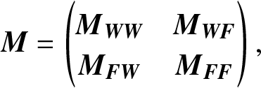 \begin{align*}
{\bf{M}} = \left(
\begin{matrix}
{{{\bf{M}}_{{\bf{WW}}}}} & {{{\bf{M}}_{{\bf{WF}}}}} \\
{{{\bf{M}}_{{\bf{FW}}}}} & {{{\bf{M}}_{{\bf{FF}}}}}
\end{matrix}
\right),
\end{align*}
\begin{align*}
{\bf{M}} = \left(
\begin{matrix}
{{{\bf{M}}_{{\bf{WW}}}}} & {{{\bf{M}}_{{\bf{WF}}}}} \\
{{{\bf{M}}_{{\bf{FW}}}}} & {{{\bf{M}}_{{\bf{FF}}}}}
\end{matrix}
\right),
\end{align*}if  ${{\bf{M}}_{{\bf{WW}}}}$ and ${{\bf{M}}_{{\bf{FF}}}}$ are not singular, as discussed in Colquhoun and Hawkes [Reference Colquhoun and Hawkes11], its inversed matrix is
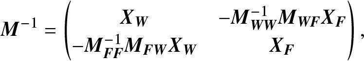 \begin{equation*}
{{\bf{M}}^{- 1}} = \left(
\begin{matrix}
{{{\bf{X}}_{\bf{W}}}} & {- {\bf{M}}_{{\bf{WW}}}^{- 1}{{\bf{M}}_{{\bf{WF}}}}{{\bf{X}}_{\bf{F}}}} \\
{- {\bf{M}}_{{\bf{FF}}}^{- 1}{{\bf{M}}_{{\bf{FW}}}}{{\bf{X}}_{\bf{W}}}} & {{{\bf{X}}_{\bf{F}}}}
\end{matrix}
\right),
\end{equation*}
\begin{equation*}
{{\bf{M}}^{- 1}} = \left(
\begin{matrix}
{{{\bf{X}}_{\bf{W}}}} & {- {\bf{M}}_{{\bf{WW}}}^{- 1}{{\bf{M}}_{{\bf{WF}}}}{{\bf{X}}_{\bf{F}}}} \\
{- {\bf{M}}_{{\bf{FF}}}^{- 1}{{\bf{M}}_{{\bf{FW}}}}{{\bf{X}}_{\bf{W}}}} & {{{\bf{X}}_{\bf{F}}}}
\end{matrix}
\right),
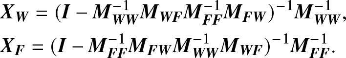
\end{equation*}where
 \begin{align*}
&{{\bf{X}}_{\bf{W}}} = {({\bf{I}} - {\bf{M}}_{{\bf{WW}}}^{- 1}{{\bf{M}}_{{\bf{WF}}}}{\bf{M}}_{{\bf{FF}}}^{- 1}{{\bf{M}}_{{\bf{FW}}}})^{- 1}}{\bf{M}}_{{\bf{WW}}}^{- 1},\\
&{{\bf{X}}_{\bf{F}}} = {({\bf{I}} - {\bf{M}}_{{\bf{FF}}}^{- 1}{{\bf{M}}_{{\bf{FW}}}}{\bf{M}}_{{\bf{WW}}}^{- 1}{{\bf{M}}_{{\bf{WF}}}})^{- 1}}{\bf{M}}_{{\bf{FF}}}^{- 1}.
\end{align*}
\begin{align*}
&{{\bf{X}}_{\bf{W}}} = {({\bf{I}} - {\bf{M}}_{{\bf{WW}}}^{- 1}{{\bf{M}}_{{\bf{WF}}}}{\bf{M}}_{{\bf{FF}}}^{- 1}{{\bf{M}}_{{\bf{FW}}}})^{- 1}}{\bf{M}}_{{\bf{WW}}}^{- 1},\\
&{{\bf{X}}_{\bf{F}}} = {({\bf{I}} - {\bf{M}}_{{\bf{FF}}}^{- 1}{{\bf{M}}_{{\bf{FW}}}}{\bf{M}}_{{\bf{WW}}}^{- 1}{{\bf{M}}_{{\bf{WF}}}})^{- 1}}{\bf{M}}_{{\bf{FF}}}^{- 1}.
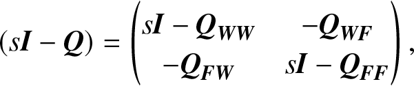
\end{align*}Using the results presented above, for
 \begin{align*}
(s{\bf{I}} - {\bf{Q}}) = \left(
\begin{matrix}
{s{\bf{I}} - {{\bf{Q}}_{{\bf{WW}}}}} & {- {{\bf{Q}}_{{\bf{WF}}}}} \\
{- {{\bf{Q}}_{{\bf{FW}}}}} & {s{\bf{I}} - {{\bf{Q}}_{{\bf{FF}}}}}
\end{matrix}
\right),
\end{align*}
\begin{align*}
(s{\bf{I}} - {\bf{Q}}) = \left(
\begin{matrix}
{s{\bf{I}} - {{\bf{Q}}_{{\bf{WW}}}}} & {- {{\bf{Q}}_{{\bf{WF}}}}} \\
{- {{\bf{Q}}_{{\bf{FW}}}}} & {s{\bf{I}} - {{\bf{Q}}_{{\bf{FF}}}}}
\end{matrix}
\right),
\end{align*}we have
 \begin{align}
{(s{\bf{I}} - {\bf{Q}})^{- 1}} = \left(
\begin{matrix}
{{{[{\bf{P}}(s)]}_{{\bf{WW}}}}} & {{{[{\bf{P}}(s)]}_{{\bf{WF}}}}} \\
{{{[{\bf{P}}(s)]}_{{\bf{FW}}}}} & {{{[{\bf{P}}(s)]}_{{\bf{FF}}}}}
\end{matrix}
\right),
\end{align}
\begin{align}
{(s{\bf{I}} - {\bf{Q}})^{- 1}} = \left(
\begin{matrix}
{{{[{\bf{P}}(s)]}_{{\bf{WW}}}}} & {{{[{\bf{P}}(s)]}_{{\bf{WF}}}}} \\
{{{[{\bf{P}}(s)]}_{{\bf{FW}}}}} & {{{[{\bf{P}}(s)]}_{{\bf{FF}}}}}
\end{matrix}
\right),
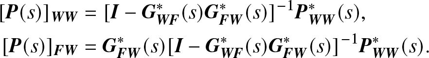
\end{align}where
 \begin{align*}
{[{\bf{P}}(s)]_{{\bf{WW}}}} &= {[{\bf{I}} - {\bf{G}}_{{\bf{WF}}}^*(s){\bf{G}}_{{\bf{FW}}}^*(s)]^{- 1}}{\bf{P}}_{{\bf{WW}}}^*(s),\\
{[{\bf{P}}(s)]_{{\bf{FW}}}} & = {\bf{G}}_{{\bf{FW}}}^*(s){[{\bf{I}} - {\bf{G}}_{{\bf{WF}}}^*(s){\bf{G}}_{{\bf{FW}}}^*(s)]^{- 1}}{\bf{P}}_{{\bf{WW}}}^*(s).
\end{align*}
\begin{align*}
{[{\bf{P}}(s)]_{{\bf{WW}}}} &= {[{\bf{I}} - {\bf{G}}_{{\bf{WF}}}^*(s){\bf{G}}_{{\bf{FW}}}^*(s)]^{- 1}}{\bf{P}}_{{\bf{WW}}}^*(s),\\
{[{\bf{P}}(s)]_{{\bf{FW}}}} & = {\bf{G}}_{{\bf{FW}}}^*(s){[{\bf{I}} - {\bf{G}}_{{\bf{WF}}}^*(s){\bf{G}}_{{\bf{FW}}}^*(s)]^{- 1}}{\bf{P}}_{{\bf{WW}}}^*(s).
\end{align*} For the results on the inversion of a partitioned matrix, there is a requirement on the existence of both matrix  ${(s{\bf{I}} - {{\bf{Q}}_{{\bf{WW}}}})^{- 1}}$ and matrix ${(s{\bf{I}} - {{\bf{Q}}_{{\bf{FF}}}})^{- 1}}$ for any variable s > 0. The proof for these can be found in several literature, for example, see Yin and Cui [Reference Yin and Cui30].
On the other hand, the existence of  ${\bf{Q}}_{{\bf{WW}}}^{- 1}$ and ${\bf{Q}}_{{\bf{FF}}}^{- 1}$ is also needed for the underlying stochastic Markov process $\{X(t),t \ge 0\} $. In the ion channel modeling literature, the time reversibility and communication for all states on the underlying process are assumed, but in our paper, it is extended into the situation of ${\rm{Rank}}({\bf{Q}}) = n - 1$, that is, the rank of transition rate matrix Q is equal to n − 1, which can not only cover the case in ion channel modeling but also include many other cases, for example, see some numerical examples presented in Section 5 of this paper. The proof of the existence of ${\bf{Q}}_{{\bf{WW}}}^{- 1}$ and ${\bf{Q}}_{{\bf{FF}}}^{- 1}$ is given in the following lemma.
Lemma 2.1. For a finite-state time-homogenous Markov process  $\{X(t),t \ge 0\} $ with transition rate matrix ${{\bf{Q}}_{n \times n}}$ and state space S, if all states communicate with each other, then ${\rm{Rank}}({{\bf{Q}}_{n \times n}}) = n - 1$ and ${\rm{Rank}}({{\bf{Q}}_{{\bf{WW}}}}) = {n_o} $, ${\rm{Rank}}({{\bf{Q}}_{{\bf{FF}}}}) = n - {n_o} $.
Proof. Let the transition rate matrix be
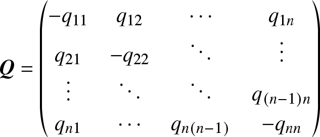 \begin{equation*}\bf Q={\left(\begin{array}{@{\kern-0.1pt}cccc@{\kern-0.1pt}}-q_{11}&q_{12}&\cdots&q_{1n}\\q_{21}&-q_{22}&\ddots&\vdots\\\vdots&\ddots&\ddots&q_{(n-1)n}\\q_{n1}&\cdots&q_{n(n-1)}&-q_{nn}\end{array}\right)}\end{equation*}
and the steady-state probability vector be  ${\bf{\pi }} = {({\pi _1},{\pi _2}, \ldots ,{\pi _n})^{\rm T}}$. Since the vector π satisfies the following set of equations
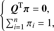 \begin{equation*}\left \{\begin{array}{@{\kern-0.1pt}c}\bf Q^{\mathrm T}\bf\pi=\mathbf0,\\\sum_{i=1}^n\pi_i=1,\end{array}\right.\end{equation*}
which is equivalent to the following linear set of equations
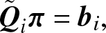 \begin{equation}
{{\tilde{\bf{Q}}}_i}{\bf{\pi }} = {{\bf{b}}_i},
\end{equation}
\begin{equation}
{{\tilde{\bf{Q}}}_i}{\bf{\pi }} = {{\bf{b}}_i},
\end{equation}where  ${{\bf{b}}_i} = {(\underbrace {0, \ldots ,0,1,}_i0, \ldots ,0)^{\rm T}}$ and
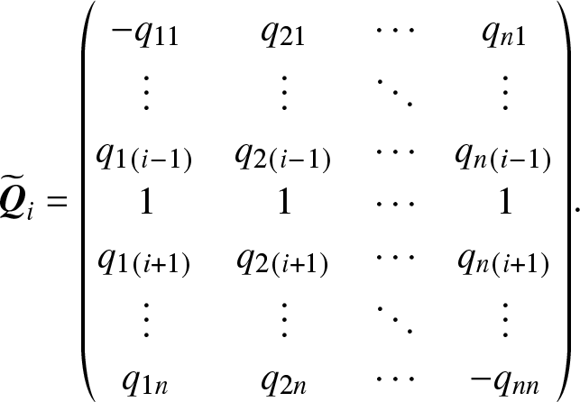 \begin{equation*}\begin{array}{rlrlrlrlrlrl}{\widetilde{\bf Q}}_i={\left(\begin{array}{@{\kern-0.1pt}cccc@{\kern-0.1pt}} -q_{11}& q_{21} & \cdots & q_{n1}\\ \vdots & \vdots & \ddots & \vdots\\ q_{1(i-1)} & q_{2(i-1)} & \cdots & q_{n(i-1)}\\ 1 & 1 & \cdots & 1\\ q_{1(i+1)} & q_{2(i+1)} & \cdots & q_{n(i+1)}\\ \vdots & \vdots & \ddots & \vdots\\ q_{1n} & q_{2n} & \cdots & -q_{nn}\end{array}\right)}.\end{array}\end{equation*}
Because we know that there exists a unique solution π to Eq. (2.10) and all πi are greater than zero in terms of all states being communicated to each other, then based on Cramer rule, we have
 \begin{align*}
&{\rm{Rank}}({{\tilde{\bf{Q}}}_i}) = {\rm{Rank}}({{\tilde{\bf{Q}}}_i};{{\bf{b}}_i}) = n, \\
&{\pi _j} = {{\det [{{{\tilde{\bf{Q}}}}_{i,j}}]} \over {\det [{{{\tilde{\bf{Q}}}}_i}]}},\quad j = 1,2, \ldots ,n,
\end{align*}
\begin{align*}
&{\rm{Rank}}({{\tilde{\bf{Q}}}_i}) = {\rm{Rank}}({{\tilde{\bf{Q}}}_i};{{\bf{b}}_i}) = n, \\
&{\pi _j} = {{\det [{{{\tilde{\bf{Q}}}}_{i,j}}]} \over {\det [{{{\tilde{\bf{Q}}}}_i}]}},\quad j = 1,2, \ldots ,n,
\end{align*}where  ${{\tilde{\bf{Q}}}_{i,j}}$ is a matrix resulting from replacing the jth column of ${{\tilde{\bf{Q}}}_i}$ by vector ${{\bf{b}}_i}$. Furthermore, we have $\det [{{\tilde{\bf{Q}}}_{i,j}}] \ne 0$ because ${\pi _j} \gt 0$, that is, ${\rm{Rank}}({{\tilde{\bf{Q}}}_{i,j}}) = n$ for any $i,j \in {\bf{S}}$. When taking $i = j = n$ as a special case, we have
 \begin{equation*}{\widetilde{\bf Q}}_{n-1,n-1}={\left(\begin{array}{@{\kern-0.1pt}cccc@{\kern-0.1pt}}-q_{11}&\cdots&q_{(n-1)1}&0\\\vdots&\ddots&\vdots&\vdots\\q_{1(n-1)}&\cdots&-q_{(n-1)(n-1)}&0\\1&\cdots&1&1\end{array}\right)}\end{equation*}
and
 \begin{equation*}\begin{array}{rlrlrlrlrlrl}\operatorname{det}{\left({\widetilde{\bf Q}}_{(n-1),(n-1)}\right)}& =\operatorname{det}{\left(\begin{array}{@{\kern-0.1pt}ccc@{\kern-0.1pt}} - q_{11} & \cdots& q_{(n-1)1}\\\vdots & \ddots & \vdots\\q_{1(n-1)} & \cdots & -q_{(n-1)(n-1)}\end{array}\right)}\\[18pt] & =\operatorname{det}{\left(\begin{array}{@{\kern-0.1pt}ccc@{\kern-0.1pt}} -q_{11} & \cdots & q_{1(n-1)}\\ \vdots& \ddots & \vdots\\ q_{(n-1)1} & \cdots & -q_{(n-1)(n-1)}\end{array}\right)}\neq 0,\end{array}\end{equation*}
that is,  ${\rm{Rank}}({\bf{Q}}) = n - 1$. Furthermore, without loss of generality, it is assumed that the state space S can be partitioned into two disjoint parts, that is, ${\bf{S}} = {\bf{W}} + {\bf{F}} = \{1,2, \ldots ,{n_o}\} + \{{n_o} + 1,{n_o} + 2, \ldots ,n\} .$ We consider the special case of $i = j = {n_o} + 1$, that is,
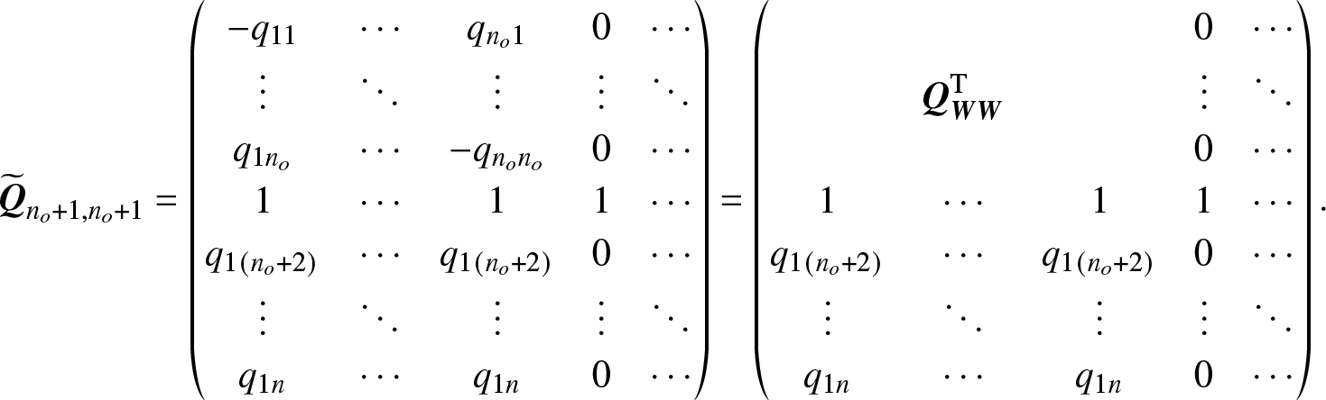 \begin{equation*}{\widetilde{\bf Q}}_{n_o+1,n_o+1}=\begin{pmatrix}-q_{11}&\cdots&q_{n_o1}&0&\cdots\\\vdots&\ddots&\vdots&\vdots&\ddots\\q_{1n_o}&\cdots&-q_{n_on_o}&0&\cdots\\1&\cdots&1&1&\cdots\\q_{1(n_o+2)}&\cdots&q_{1(n_o+2)}&0&\cdots\\\vdots&\ddots&\vdots&\vdots&\ddots\\q_{1n}&\cdots&q_{1n}&0&\cdots\end{pmatrix}=\begin{pmatrix}&&&0&\cdots\\&\bf Q_{\bf W\bf W}^{\mathrm T}&&\vdots&\ddots\\&&&0&\cdots\\1&\cdots&1&1&\cdots\\q_{1(n_o+2)}&\cdots&q_{1(n_o+2)}&0&\cdots\\\vdots&\ddots&\vdots&\vdots&\ddots\\q_{1n}&\cdots&q_{1n}&0&\cdots\end{pmatrix}.\end{equation*}
 Thus, we have  $\det [{\bf{Q}}_{{\bf{WW}}}^{\rm T}] = \det [{{\bf{Q}}_{{\bf{WW}}}}] \ne 0$, that is to say, ${\rm{Rank}}({{\bf{Q}}_{{\bf{WW}}}}) = {n_o} = |{\bf{W}}|$. Similarly, we can prove that ${\rm{Rank}}({{\bf{Q}}_{{\bf{FF}}}}) = n - {n_o} = |{\bf{F}}|$. It completes the proof.
As mentioned above, if  ${\rm{Rank}}({{\bf{Q}}_{n \times n}}) = n - 1$ for a finite-state time-homogenous Markov process, all states may communicate or not, for example, see examples presented in Section 5. On the other hand, Lemma 2.1 told us that if all states communicate with each other in a finite state Markov process, then the rank of its transition rate matrix is n − 1.
Unlike in the ion channel modeling, in this paper, we focus on the limiting behaviors of the aggregated Markov processes, which are used to describe the maintenance processes in the reliability field. The four steady-state reliability indexes are studied, which include the steady-state availability, the steady-state interval availability, the steady-state transition probability between two subsets, and the steady-state probability staying at a subset. All these four indexes can be expressed through using the aggregated Markov process and the initial conditions of the underlying process being at the initial time t = 0, which all are the products of the initial probability vectors and matrices. It is not easy to know directly in terms of these formulas that these expressions do not depend on the initial probability vectors. However, the common knowledge in Markov processes tells us that they hold true. The proofs on that will be presented in terms of these products when time approaches to infinity in next section.
3. Limiting results derived by using aggregated Markov processes
The limiting results in aggregated stochastic processes are considered in many theoretical and practical situations. In reliability field, especially for repairable systems, some limiting behaviors need to be considered. The following four reliability-related measures, in general, are paid attention to:
(1) the steady-state availability, denoted as $\mathop {\lim }\limits_{t \to \infty } A(t)$;
(2) the steady-state interval availability, denoted as
$\mathop {\lim }\limits_{t \to \infty } A([t,t + a])$, where $a \ge 0$;(3) the steady-state transition probability between two subsets, denoted as
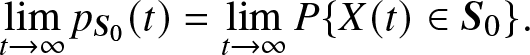
$\mathop {\lim }\limits_{t \to \infty } {p_{{{\bf{S}}_1}{{\bf{S}}_2}}}(t)$, where ${{\bf{S}}_i} \subsetneq {\bf{S}}$, $(i = 1,2)$ and ${{\bf{S}}_1} \cap {{\bf{S}}_2} = \phi $, ϕ is an empty set; and(4) the steady-state probability staying in a given subset
$\mathop {\lim }\limits_{t \to \infty } {p_{{{\bf{S}}_0}}}(t)$, where ${{\bf{S}}_0} \subsetneq {\bf{S}}$, that is, ${{\bf{S}}_0}$ is a proper subset of state space S.


In the sequeal, the computation formulas for the four measures are derived in terms of the theory of aggregated Markov processes.
(1) The steady-state availability
The definition of steady-state availability is given by
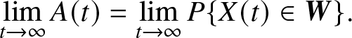 \begin{equation}
\mathop {\lim }\limits_{t \to \infty } A(t) = \mathop {\lim }\limits_{t \to \infty } P\{X(t) \in {\bf{W}}\} .
\end{equation}
\begin{equation}
\mathop {\lim }\limits_{t \to \infty } A(t) = \mathop {\lim }\limits_{t \to \infty } P\{X(t) \in {\bf{W}}\} .
\end{equation} Let  ${\bf{A}}(t) = ({A_1}(t), \ldots ,{A_{|{\bf{W}}|}}(t))$, where ${A_i}(t) = P\{X(t) = i \in {\bf{W}}\} $, then we have
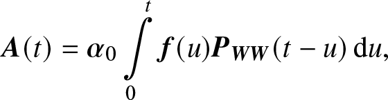 \begin{equation}
{\bf{A}}(t) = {{\bf{\alpha }}_0}\int\limits_0^t {{\bf{f}}(u){{\bf{P}}_{{\bf{WW}}}}(t - u)\,{\rm{d}}u},
\end{equation}
\begin{equation}
{\bf{A}}(t) = {{\bf{\alpha }}_0}\int\limits_0^t {{\bf{f}}(u){{\bf{P}}_{{\bf{WW}}}}(t - u)\,{\rm{d}}u},
\end{equation}where  ${{\bf{P}}_{{\bf{WW}}}}(t) = \exp ({{\bf{Q}}_{{\bf{WW}}}}t)$ and ${\bf{f}}(t) = {\left( {{f_{ij}}(t)} \right)_{|{\bf{S}}| \times |{\bf{W}}|}}$, its elements ${f_{ij}}(t)$ are the probability density functions of the durations starting from state i at time 0 and ending at time t by entering state j, with initial probability vector ${{\bf{\alpha }}_0} = ({{\bf{\alpha }}_{\bf{W}}},{{\bf{\alpha }}_{\bf{F}}})$. Thus, the Laplace transform of ${\bf{A}}(t)$ is
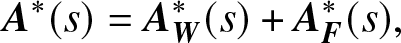 \begin{equation}
{{\bf{A}}^*}(s) = {\bf{A}}_{\bf{W}}^*(s) + {\bf{A}}_{\bf{F}}^*(s),
\end{equation}
\begin{equation}
{{\bf{A}}^*}(s) = {\bf{A}}_{\bf{W}}^*(s) + {\bf{A}}_{\bf{F}}^*(s),
\end{equation}where  ${A_{\bf{W}}}(t): = P\{X(t) \in {\bf{W}}\} $ and ${A_{\bf{F}}}(t): = P\{X(t) \in {\bf{F}}\} $,
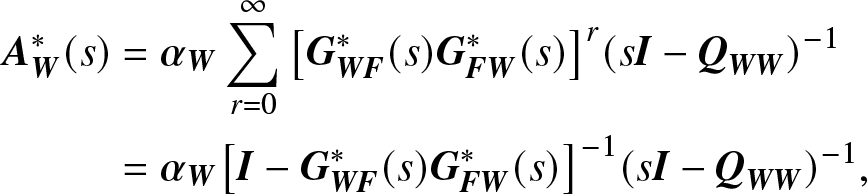 \begin{align}
{\bf{A}}_{\bf{W}}^*(s)& = {{\bf{\alpha }}_{\bf{W}}}\sum\limits_{r = 0}^\infty {{{\left[{\bf{G}}_{{\bf{WF}}}^*(s){\bf{G}}_{{\bf{FW}}}^*(s)\right]}^r}} {(s{\bf{I}} - {{\bf{Q}}_{{\bf{WW}}}})^{- 1}}\notag \\
& = {{\bf{\alpha }}_{\bf{W}}}{\left[{\bf{I}} - {\bf{G}}_{{\bf{WF}}}^*(s){\bf{G}}_{{\bf{FW}}}^*(s)\right]^{- 1}}{(s{\bf{I}} - {{\bf{Q}}_{{\bf{WW}}}})^{- 1}} ,
\end{align}
\begin{align}
{\bf{A}}_{\bf{W}}^*(s)& = {{\bf{\alpha }}_{\bf{W}}}\sum\limits_{r = 0}^\infty {{{\left[{\bf{G}}_{{\bf{WF}}}^*(s){\bf{G}}_{{\bf{FW}}}^*(s)\right]}^r}} {(s{\bf{I}} - {{\bf{Q}}_{{\bf{WW}}}})^{- 1}}\notag \\
& = {{\bf{\alpha }}_{\bf{W}}}{\left[{\bf{I}} - {\bf{G}}_{{\bf{WF}}}^*(s){\bf{G}}_{{\bf{FW}}}^*(s)\right]^{- 1}}{(s{\bf{I}} - {{\bf{Q}}_{{\bf{WW}}}})^{- 1}} ,
\end{align}this is because the system is in W at time t after it spends a duration of either 0, or 1, or 2,  $\ldots$ transitions from W to F and back, and the convolution forms a product by taking the Laplace transform. Similarly, we have
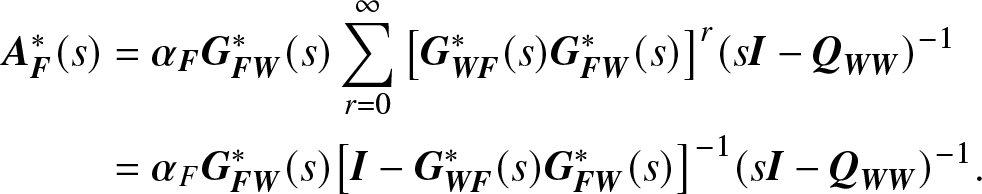
 \begin{align}
{\bf{A}}_{\bf{F}}^*(s)& = {{\bf{\alpha }}_{\bf{F}}}{\bf{G}}_{{\bf{FW}}}^*(s)\sum\limits_{r = 0}^\infty {{{\left[{\bf{G}}_{{\bf{WF}}}^*(s){\bf{G}}_{{\bf{FW}}}^*(s)\right]}^r}} {(s{\bf{I}} - {{\bf{Q}}_{{\bf{WW}}}})^{- 1}}\notag \\
& = {{\bf{\alpha }}_F} {\bf{G}}_{{\bf{FW}}}^*(s){\left[{\bf{I}} - {\bf{G}}_{{\bf{WF}}}^*(s){\bf{G}}_{{\bf{FW}}}^*(s)\right]^{- 1}}{(s{\bf{I}} - {{\bf{Q}}_{{\bf{WW}}}})^{- 1}}.
\end{align}
\begin{align}
{\bf{A}}_{\bf{F}}^*(s)& = {{\bf{\alpha }}_{\bf{F}}}{\bf{G}}_{{\bf{FW}}}^*(s)\sum\limits_{r = 0}^\infty {{{\left[{\bf{G}}_{{\bf{WF}}}^*(s){\bf{G}}_{{\bf{FW}}}^*(s)\right]}^r}} {(s{\bf{I}} - {{\bf{Q}}_{{\bf{WW}}}})^{- 1}}\notag \\
& = {{\bf{\alpha }}_F} {\bf{G}}_{{\bf{FW}}}^*(s){\left[{\bf{I}} - {\bf{G}}_{{\bf{WF}}}^*(s){\bf{G}}_{{\bf{FW}}}^*(s)\right]^{- 1}}{(s{\bf{I}} - {{\bf{Q}}_{{\bf{WW}}}})^{- 1}}.
\end{align}Based on Tauber’s Theorem ([Reference Korevaar22], Final Value Theorem [Reference Cohen9]), Theorem 14.1 in reference [Reference Korevaar22], or Theorem 2.6 in reference [Reference Cohen9] tells us that
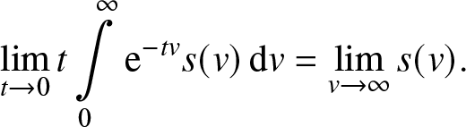 \begin{equation*}\mathop {\lim }\limits_{t \to 0} t\int\limits_0^\infty {{{\rm e}^{- tv}}} s(v)\,{\rm{d}}v = \mathop {\lim }\limits_{v \to \infty } s(v).\end{equation*}
Then, we have
 \begin{equation}
\mathop {\lim }\limits_{t \to \infty } A(t) = \mathop {\lim }\limits_{t \to \infty } [({{\bf{A}}_W}(t) + {{\bf{A}}_F}(t)){{\bf{u}}_{\bf{W}}}] = \mathop {\lim }\limits_{s \downarrow 0} [s({\bf{A}}_W^*(s) + {\bf{A}}_F^*(s)){{\bf{u}}_{\bf{W}}}],
\end{equation}
\begin{equation}
\mathop {\lim }\limits_{t \to \infty } A(t) = \mathop {\lim }\limits_{t \to \infty } [({{\bf{A}}_W}(t) + {{\bf{A}}_F}(t)){{\bf{u}}_{\bf{W}}}] = \mathop {\lim }\limits_{s \downarrow 0} [s({\bf{A}}_W^*(s) + {\bf{A}}_F^*(s)){{\bf{u}}_{\bf{W}}}],
\end{equation}where  ${{\bf{u}}_{\bf{W}}} = (\underbrace {1, \ldots ,1}_{\left| {\bf{W}} \right|})^{\rm T}$.
(2) The steady-state interval availability  $\mathop {\lim }\limits_{t \to \infty } A([t,t + a])$
The definition of steady-state interval availability is given by
 \begin{equation}
\mathop {\lim }\limits_{t \to \infty } A([t,t + a]) = \mathop {\lim }\limits_{t \to \infty } P\{X(u) \in {\bf{W}}, {\rm{~for~all~}}u \in [t,t + a]\}.
\end{equation}
\begin{equation}
\mathop {\lim }\limits_{t \to \infty } A([t,t + a]) = \mathop {\lim }\limits_{t \to \infty } P\{X(u) \in {\bf{W}}, {\rm{~for~all~}}u \in [t,t + a]\}.
\end{equation} Since  $A([t,t + a]) = {{\bf{A}}_{\bf{W}}}(t)\,\exp (a{{\bf{Q}}_{{\bf{WW}}}}){{\bf{u}}_{\bf{W}}}$, thus we have
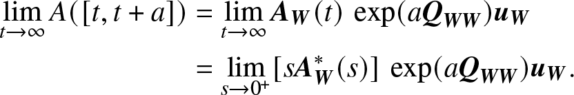 \begin{align}
\mathop {\lim }\limits_{t \to \infty } A([t,t + a]) &= \mathop {\lim }\limits_{t \to \infty } {{\bf{A}}_{\bf{W}}}(t)\,\exp (a{{\bf{Q}}_{{\bf{WW}}}}){{\bf{u}}_{\bf{W}}}\notag \\
&= \mathop {\lim }\limits_{s \to {0^ + }} [s{\bf{A}}_{\bf{W}}^*(s)]\,\exp (a{{\bf{Q}}_{{\bf{WW}}}}){{\bf{u}}_{\bf{W}}}.
\end{align}
\begin{align}
\mathop {\lim }\limits_{t \to \infty } A([t,t + a]) &= \mathop {\lim }\limits_{t \to \infty } {{\bf{A}}_{\bf{W}}}(t)\,\exp (a{{\bf{Q}}_{{\bf{WW}}}}){{\bf{u}}_{\bf{W}}}\notag \\
&= \mathop {\lim }\limits_{s \to {0^ + }} [s{\bf{A}}_{\bf{W}}^*(s)]\,\exp (a{{\bf{Q}}_{{\bf{WW}}}}){{\bf{u}}_{\bf{W}}}.
\end{align} (3) The steady-state transition probability between two subsets  $\mathop {\lim }\limits_{t \to \infty } {p_{{{\bf{S}}_1}{{\bf{S}}_2}}}(t)$
The definition of steady-state transition probability between two subsets is given by
 \begin{equation}
\mathop {\lim }\limits_{t \to \infty } {p_{{{\bf{S}}_1}{{\bf{S}}_2}}}(t) = \mathop {\lim }\limits_{t \to \infty } P\{X(t) \in {{\bf{S}}_2}|X(0) \in {{\bf{S}}_1}\}.
\end{equation}
\begin{equation}
\mathop {\lim }\limits_{t \to \infty } {p_{{{\bf{S}}_1}{{\bf{S}}_2}}}(t) = \mathop {\lim }\limits_{t \to \infty } P\{X(t) \in {{\bf{S}}_2}|X(0) \in {{\bf{S}}_1}\}.
\end{equation}There are two cases to be considered in the following:
Case 1:  ${{\bf{S}}_1} \cup {{\bf{S}}_2} = {\bf{S}}$
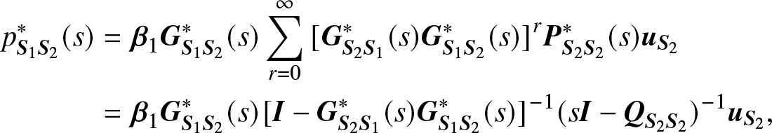 \begin{align}
p_{{{\bf{S}}_1}{{\bf{S}}_2}}^*(s) &= {{\bf{\beta }}_1}{\bf{G}}_{{{\bf{S}}_1}{{\bf{S}}_2}}^*(s)\sum\limits_{r = 0}^\infty {{{[{\bf{G}}_{{{\bf{S}}_2}{{\bf{S}}_1}}^*(s){\bf{G}}_{{{\bf{S}}_1}{{\bf{S}}_2}}^*(s)]}^r}} {\bf{P}}_{{{\bf{S}}_2}{{\bf{S}}_2}}^*(s){{\bf{u}}_{{{\bf{S}}_2}}} \notag \\
& = {{\bf{\beta }}_1}{\bf{G}}_{{{\bf{S}}_1}{{\bf{S}}_2}}^*(s){[{\bf{I}} - {\bf{G}}_{{{\bf{S}}_2}{{\bf{S}}_1}}^*(s){\bf{G}}_{{{\bf{S}}_1}{{\bf{S}}_2}}^*(s)]^{- 1}}{(s{\bf{I}} - {{\bf{Q}}_{{{\bf{S}}_2}{{\bf{S}}_2}}})^{- 1}}{{\bf{u}}_{{{\bf{S}}_2}}},
\end{align}
\begin{align}
p_{{{\bf{S}}_1}{{\bf{S}}_2}}^*(s) &= {{\bf{\beta }}_1}{\bf{G}}_{{{\bf{S}}_1}{{\bf{S}}_2}}^*(s)\sum\limits_{r = 0}^\infty {{{[{\bf{G}}_{{{\bf{S}}_2}{{\bf{S}}_1}}^*(s){\bf{G}}_{{{\bf{S}}_1}{{\bf{S}}_2}}^*(s)]}^r}} {\bf{P}}_{{{\bf{S}}_2}{{\bf{S}}_2}}^*(s){{\bf{u}}_{{{\bf{S}}_2}}} \notag \\
& = {{\bf{\beta }}_1}{\bf{G}}_{{{\bf{S}}_1}{{\bf{S}}_2}}^*(s){[{\bf{I}} - {\bf{G}}_{{{\bf{S}}_2}{{\bf{S}}_1}}^*(s){\bf{G}}_{{{\bf{S}}_1}{{\bf{S}}_2}}^*(s)]^{- 1}}{(s{\bf{I}} - {{\bf{Q}}_{{{\bf{S}}_2}{{\bf{S}}_2}}})^{- 1}}{{\bf{u}}_{{{\bf{S}}_2}}},
\end{align}where the initial probability vector  ${{\bf{\beta }}_1} = \left({{{\alpha _1}} \over {\sum\limits_{i \in {{\bf{S}}_1}} {{\alpha _i}} }}, \ldots ,{{{\alpha _{|{{\bf{S}}_1}|}}} \over {\sum\limits_{i \in {{\bf{S}}_1}} {{\alpha _i}} }}\right): = ({\beta _1}, \ldots ,{\beta _{|{{\bf{S}}_1}|}})$ and ${{\bf{u}}_{{{\bf{S}}_2}}} = (\underbrace {1, \ldots ,1}_{\left| {{{\bf{S}}_2}} \right|})$.
Case 2:  ${{\bf{S}}_1} + {{\bf{S}}_2} \subsetneq {\bf{S}}$
Let  ${{\bar{\bf{S}}}_1} = {\bf{S}}/{{\bf{S}}_1}$, then we first consider the $p_{{{\bf{S}}_1}{{{\bf{\bar S}}}_1}}^*(s)$. From Case 1, we have known that
 \begin{equation*}
p_{{{\bf{S}}_1}{{{\bar{\bf{S}}}}_1}}^*(s) = {{\bf{\beta }}_1}{\bf{G}}_{{{\bf{S}}_1}{{{\bf{\bar S}}}_1}}^*(s){[{\bf{I}} - {\bf{G}}_{{{{\bf{\bar S}}}_1}{{\bf{S}}_1}}^*(s){\bf{G}}_{{{\bf{S}}_1}{{{\bf{\bar S}}}_1}}^*(s)]^{- 1}}{(s{\bf{I}} - {{\bf{Q}}_{{{{\bf{\bar S}}}_1}{{{\bf{\bar S}}}_1}}})^{- 1}}{{\bf{u}}_{{{{\bf{\bar S}}}_1}}},
\end{equation*}
\begin{equation*}
p_{{{\bf{S}}_1}{{{\bar{\bf{S}}}}_1}}^*(s) = {{\bf{\beta }}_1}{\bf{G}}_{{{\bf{S}}_1}{{{\bf{\bar S}}}_1}}^*(s){[{\bf{I}} - {\bf{G}}_{{{{\bf{\bar S}}}_1}{{\bf{S}}_1}}^*(s){\bf{G}}_{{{\bf{S}}_1}{{{\bf{\bar S}}}_1}}^*(s)]^{- 1}}{(s{\bf{I}} - {{\bf{Q}}_{{{{\bf{\bar S}}}_1}{{{\bf{\bar S}}}_1}}})^{- 1}}{{\bf{u}}_{{{{\bf{\bar S}}}_1}}},
\end{equation*}where  ${{\bf{u}}_{{{{\bf{\bar S}}}_1}}}=(\underbrace {1, \ldots ,1}_{\left| {{{{\bar{\bf{S}}}}_1}} \right|})$. On the other hand, we have
 \begin{equation}
p_{{{\bf{S}}_1}{{\bf{S}}_2}}^*(s) = {{{\bf{\beta }}_1}{\bf{G}}_{{{\bf{S}}_1}{{{\bf{\bar S}}}_1}}^*(s){[{\bf{I}} - {\bf{G}}_{{{{\bf{\bar S}}}_1}{{\bf{S}}_1}}^*(s){\bf{G}}_{{{\bf{S}}_1}{{{\bar{\bf{S}}}}_1}}^*(s)]^{- 1}}{(s{\bf{I}} - {{\bf{Q}}_{{{{\bar{\bf{S}}}}_1}{{{\bar{\bf{S}}}}_1}}})^{- 1}}{{\bf{v}}_1}},
\end{equation}
\begin{equation}
p_{{{\bf{S}}_1}{{\bf{S}}_2}}^*(s) = {{{\bf{\beta }}_1}{\bf{G}}_{{{\bf{S}}_1}{{{\bf{\bar S}}}_1}}^*(s){[{\bf{I}} - {\bf{G}}_{{{{\bf{\bar S}}}_1}{{\bf{S}}_1}}^*(s){\bf{G}}_{{{\bf{S}}_1}{{{\bar{\bf{S}}}}_1}}^*(s)]^{- 1}}{(s{\bf{I}} - {{\bf{Q}}_{{{{\bar{\bf{S}}}}_1}{{{\bar{\bf{S}}}}_1}}})^{- 1}}{{\bf{v}}_1}},
\end{equation}where  ${{\bf{v}}_1} = {(\underbrace {1, \ldots ,1}_{\left| {{S_2}} \right|},\underbrace {0, \ldots ,0}_{\left| {{{\bar S}_1}} \right| - \left| {{S_2}} \right|})^{\rm T}}$, with ${{\bf{S}}_2} \subsetneq {{\bar{\bf{S}}}_1}$.
(4) The steady-state probability staying in a given subset  $\mathop {\lim }\limits_{t \to \infty } {p_{{{\bf{S}}_0}}}(t)$
The definition of steady-state probability staying in a given subset is given by
 \begin{equation}
\mathop {\lim }\limits_{t \to \infty } {p_{{{\bf{S}}_0}}}(t) = \mathop {\lim }\limits_{t \to \infty } P\{X(t) \in {{\bf{S}}_0}\}.
\end{equation}
\begin{equation}
\mathop {\lim }\limits_{t \to \infty } {p_{{{\bf{S}}_0}}}(t) = \mathop {\lim }\limits_{t \to \infty } P\{X(t) \in {{\bf{S}}_0}\}.
\end{equation} Note: When  ${\bf{S}}_1 = {\bf{S}}$, $\mathop {\lim }\limits_{t \to \infty } {p_{{{\bf{S}}_1}{{\bf{S}}_2}}}(t)$ in Eq. (3.9) reduces to $\mathop {\lim }\limits_{t \to \infty } {p_{{{\bf{S}}_0}}}(t)$ in Eq. (3.12).
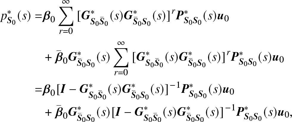
We have
 \begin{align}
p_{{{\bf{S}}_0}}^*(s) =& {{\bf{\beta }}_0}\sum\limits_{r = 0}^\infty {{{[{\bf{G}}_{{{\bf{S}}_0}{{{\bar{\bf{S}}}}_0}}^*(s){\bf{G}}_{{{{\bar{\bf{S}}}}_0}{{\bf{S}}_0}}^*(s)]}^r}} {\bf{P}}_{{{\bf{S}}_0}{{\bf{S}}_0}}^*(s){{\bf{u}}_0}\notag\\
& + {{{\bar{\bf{\beta}}}}_0}{\bf{G}}_{{{{\bar{\bf{S}}}}_0}{{\bf{S}}_0}}^*(s)\sum\limits_{r = 0}^\infty {{{[{\bf{G}}_{{{\bf{S}}_0}{{{\bar{\bf{S}}}}_0}}^*(s){\bf{G}}_{{{{\bar{\bf{S}}}}_0}{{\bf{S}}_0}}^*(s)]}^r}} {\bf{P}}_{{{\bf{S}}_0}{{\bf{S}}_0}}^*(s){{\bf{u}}_0} \notag \\
=& {{\bf{\beta }}_0}{[{\bf{I}} - {\bf{G}}_{{{\bf{S}}_0}{{{\bar{\bf{S}}}}_0}}^*(s){\bf{G}}_{{{{\bar{\bf{S}}}}_0}{{\bf{S}}_0}}^*(s)]^{- 1}}{\bf{P}}_{{{\bf{S}}_0}{{\bf{S}}_0}}^*(s){{\bf{u}}_0} \notag\\
&+ {{{\bar{\bf{\beta}}}}_0}{\bf{G}}_{{{{\bar{\bf{S}}}}_0}{{\bf{S}}_0}}^*(s){[{\bf{I}} - {\bf{G}}_{{{\bf{S}}_0}{{{\bar{\bf{S}}}}_0}}^*(s){\bf{G}}_{{{{\bar{\bf{S}}}}_0}{{\bf{S}}_0}}^*(s)]^{- 1}}{\bf{P}}_{{{\bf{S}}_0}{{\bf{S}}_0}}^*(s){{\bf{u}}_0},
\end{align}
\begin{align}
p_{{{\bf{S}}_0}}^*(s) =& {{\bf{\beta }}_0}\sum\limits_{r = 0}^\infty {{{[{\bf{G}}_{{{\bf{S}}_0}{{{\bar{\bf{S}}}}_0}}^*(s){\bf{G}}_{{{{\bar{\bf{S}}}}_0}{{\bf{S}}_0}}^*(s)]}^r}} {\bf{P}}_{{{\bf{S}}_0}{{\bf{S}}_0}}^*(s){{\bf{u}}_0}\notag\\
& + {{{\bar{\bf{\beta}}}}_0}{\bf{G}}_{{{{\bar{\bf{S}}}}_0}{{\bf{S}}_0}}^*(s)\sum\limits_{r = 0}^\infty {{{[{\bf{G}}_{{{\bf{S}}_0}{{{\bar{\bf{S}}}}_0}}^*(s){\bf{G}}_{{{{\bar{\bf{S}}}}_0}{{\bf{S}}_0}}^*(s)]}^r}} {\bf{P}}_{{{\bf{S}}_0}{{\bf{S}}_0}}^*(s){{\bf{u}}_0} \notag \\
=& {{\bf{\beta }}_0}{[{\bf{I}} - {\bf{G}}_{{{\bf{S}}_0}{{{\bar{\bf{S}}}}_0}}^*(s){\bf{G}}_{{{{\bar{\bf{S}}}}_0}{{\bf{S}}_0}}^*(s)]^{- 1}}{\bf{P}}_{{{\bf{S}}_0}{{\bf{S}}_0}}^*(s){{\bf{u}}_0} \notag\\
&+ {{{\bar{\bf{\beta}}}}_0}{\bf{G}}_{{{{\bar{\bf{S}}}}_0}{{\bf{S}}_0}}^*(s){[{\bf{I}} - {\bf{G}}_{{{\bf{S}}_0}{{{\bar{\bf{S}}}}_0}}^*(s){\bf{G}}_{{{{\bar{\bf{S}}}}_0}{{\bf{S}}_0}}^*(s)]^{- 1}}{\bf{P}}_{{{\bf{S}}_0}{{\bf{S}}_0}}^*(s){{\bf{u}}_0},
\end{align}where the initial probability vectors  ${{\bf{\beta }}_0} = ({\alpha _1}, \ldots ,{\alpha _{|{{\bf{S}}_0}|}})$, ${{\bar{\bf{\beta}}}_0} = ({\alpha _{|{{\bf{S}}_0}| + 1}}, \ldots ,{\alpha _{|{\bf{S}}|}})$, and ${{\bf{u}}_0} = (\underbrace {1, \ldots ,1}_{\left| {{{\bf{S}}_0}} \right|})^{\rm T}$.
Note: In some contents, the steady-state probability staying at a given subset  $\mathop {\lim }\limits_{t \to \infty } {p_{{{\bf{S}}_0}}}(t)$ is equivalent to the steady-state availability $\mathop {\lim }\limits_{t \to \infty } A(t)$ when two subsets coincide, that is, $\mathop {\lim }\limits_{t \to \infty } {p_{{{\bf{S}}_0}}}(t) = \mathop {\lim }\limits_{t \to \infty } A(t)$ when ${\bf{W}} = {{\bf{S}}_0}$.
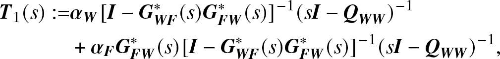
Based on the four steady-state measures expressed by Eqs. (3.5), (3.6), (3.8), (3.10), (3.11), and (3.13), we only need to consider essentially two terms, which are
 \begin{align}
{{\bf{T}}_1}(s): =& {{\bf{\alpha }}_{\bf{W}}}{[{\bf{I}} - {\bf{G}}_{{\bf{WF}}}^*(s){\bf{G}}_{{\bf{FW}}}^*(s)]^{- 1}}{(s{\bf{I}} - {{\bf{Q}}_{{\bf{WW}}}})^{- 1}} \notag \\
& + {{\bf{\alpha }}_{\bf{F}}} {\bf{G}}_{{\bf{FW}}}^*(s){[{\bf{I}} - {\bf{G}}_{{\bf{WF}}}^*(s){\bf{G}}_{{\bf{FW}}}^*(s)]^{- 1}}{(s{\bf{I}} - {{\bf{Q}}_{{\bf{WW}}}})^{- 1}},
\end{align}
\begin{align}
{{\bf{T}}_1}(s): =& {{\bf{\alpha }}_{\bf{W}}}{[{\bf{I}} - {\bf{G}}_{{\bf{WF}}}^*(s){\bf{G}}_{{\bf{FW}}}^*(s)]^{- 1}}{(s{\bf{I}} - {{\bf{Q}}_{{\bf{WW}}}})^{- 1}} \notag \\
& + {{\bf{\alpha }}_{\bf{F}}} {\bf{G}}_{{\bf{FW}}}^*(s){[{\bf{I}} - {\bf{G}}_{{\bf{WF}}}^*(s){\bf{G}}_{{\bf{FW}}}^*(s)]^{- 1}}{(s{\bf{I}} - {{\bf{Q}}_{{\bf{WW}}}})^{- 1}},
\end{align} \begin{align}
{{\bf{T}}_2}(s): = {{\bf{\beta }}_1}{\bf{G}}_{{\bf{FW}}}^*(s){[{\bf{I}} - {\bf{G}}_{{\bf{WF}}}^*(s){\bf{G}}_{{\bf{FW}}}^*(s)]^{- 1}}{(s{\bf{I}} - {{\bf{Q}}_{{\bf{WW}}}})^{- 1}}.
\end{align}
\begin{align}
{{\bf{T}}_2}(s): = {{\bf{\beta }}_1}{\bf{G}}_{{\bf{FW}}}^*(s){[{\bf{I}} - {\bf{G}}_{{\bf{WF}}}^*(s){\bf{G}}_{{\bf{FW}}}^*(s)]^{- 1}}{(s{\bf{I}} - {{\bf{Q}}_{{\bf{WW}}}})^{- 1}}.
\end{align} Note: when we replace the subsets  ${{\bf{S}}_1}$ and ${{\bf{S}}_2}$, ${{\bf{S}}_1}$ and ${{\bar{\bf{S}}}_1}$, ${{\bf{S}}_0}$ and ${{\bar{\bf{S}}}_0}$ by F and W in the corresponding equations, respectively, then the two terms presented in Eqs. (3.14) and (3.15) are given.
Summarizing the above cases, we need to calculate the following two limits:  $\mathop {\lim }\limits_{s \downarrow 0} [s{{\bf{T}}_i}(s)]$ $ (i = 1,2)$ for getting the four steady-state measures under the case that s approaches to zero from the right side, which is equivalent to the case that time t approaches to infinity.
4. Proofs on the limiting results
As mentioned above, the four limits do not depend on the initial state probability vector of the underlying Markov process considered, which is a well-known result in Markov processes. However, when using the results in aggregated stochastic process, it is not directly known that the four limits are not relevant to the initial state probability vector. In the following, we present a detailed proof on this conclusion. Before giving the main results, two Lemmas are needed first.
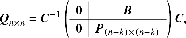
Lemma 4.1. Given a matrix  ${{\bf{Q}}_{n \times n}}$, if ${\rm{Rank}}({{\bf{Q}}_{n \times n}}) = n - k$ $(k \in \{1,2, \ldots ,n - 1\} )$, then there exists a nonsingular matrix C such that
 \begin{equation}
{{\bf{Q}}_{n \times n}} = {{\bf{C}}^{- 1}}\left(
\begin{array}{c|c}
{\bf{0}} &{\bf{B}} \\ \hline
{\bf{0}} & {{{\bf{P}}_{(n - k) \times (n - k)}}}
\end{array}
\right){\bf{C}},
\end{equation}
\begin{equation}
{{\bf{Q}}_{n \times n}} = {{\bf{C}}^{- 1}}\left(
\begin{array}{c|c}
{\bf{0}} &{\bf{B}} \\ \hline
{\bf{0}} & {{{\bf{P}}_{(n - k) \times (n - k)}}}
\end{array}
\right){\bf{C}},
\end{equation}where  ${\rm{Rank}}({{\bf{P}}_{(n - k) \times (n - k)}}) = n - k$.
Proof. See Fang et al. [Reference Fang, Zhou and Li17] .
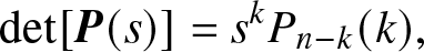
Corollary 4.1. Let matrix  ${\bf{P}}(s): = s{\bf{I}} - {\bf{Q}}$ and ${\rm{Rank}}({\bf{Q}}) = n - k$ $(k \in \{1,2, \ldots ,n - 1\} )$, where Q is the transition rate matrix of Markov process $\{X(t),t \ge 0\} $ with state space ${\bf{S}} = \{1,2, \ldots ,n\} $, then
 \begin{equation}
\det [{\bf{P}}(s)] = {s^k}{P_{n - k}}(k),
\end{equation}
\begin{equation}
\det [{\bf{P}}(s)] = {s^k}{P_{n - k}}(k),
\end{equation}where  ${P_{n - k}}(s)$ is a polynomial of s with degree n − k and ${P_{n - k}}(0) \ne 0$.
Proof. Based on Lemma 4.1, we have
 \begin{equation*}\begin{array}{rlrlrlrlrlrl}\operatorname{det}\lbrack\bf P(s)\rbrack&=\operatorname{det}\left[{s\bf I-\bf C^{-1}\left(\begin{array}{c|c}\mathbf0&\bf B\\\hline\mathbf0&{\bf P}_{(n-k)\times(n-k)}\end{array}\right)\bf C}\right]\\[12pt]
&=\operatorname{det}\left[{\bf C^{-1}\left(s\bf I-{\left(\begin{array}{c|c}\mathbf0&\bf B\\\hline\mathbf0&{\bf P}_{(n-k)\times(n-k)}\end{array}\right)}\right)\bf C}\right]\end{array}\end{equation*}
\begin{equation*}\begin{array}{rlrlrlrlrlrl}\operatorname{det}\lbrack\bf P(s)\rbrack&=\operatorname{det}\left[{s\bf I-\bf C^{-1}\left(\begin{array}{c|c}\mathbf0&\bf B\\\hline\mathbf0&{\bf P}_{(n-k)\times(n-k)}\end{array}\right)\bf C}\right]\\[12pt]
&=\operatorname{det}\left[{\bf C^{-1}\left(s\bf I-{\left(\begin{array}{c|c}\mathbf0&\bf B\\\hline\mathbf0&{\bf P}_{(n-k)\times(n-k)}\end{array}\right)}\right)\bf C}\right]\end{array}\end{equation*} \begin{equation*}\begin{array}{rlrlrlrlrlrl}&=\operatorname{det}{\left[ s\bf I-{\left(\begin{array}{c|c}\mathbf0&\bf B\\\hline\mathbf0&{\bf P}_{(n-k)\times(n-k)}\end{array}\right)}\right]}\\[12pt]&
=\operatorname{det}{\left[{\left(\begin{array}{ccc|c}s&&\mathbf0&\\&\ddots&&-\bf B\\\mathbf0&&s&\\\hline&\mathbf0&&s\bf I-{\bf P}_{(n-k)\times(n-k)}\end{array}\right)}\right]}=s^kP_{n-k}(s).\end{array}\end{equation*}
\begin{equation*}\begin{array}{rlrlrlrlrlrl}&=\operatorname{det}{\left[ s\bf I-{\left(\begin{array}{c|c}\mathbf0&\bf B\\\hline\mathbf0&{\bf P}_{(n-k)\times(n-k)}\end{array}\right)}\right]}\\[12pt]&
=\operatorname{det}{\left[{\left(\begin{array}{ccc|c}s&&\mathbf0&\\&\ddots&&-\bf B\\\mathbf0&&s&\\\hline&\mathbf0&&s\bf I-{\bf P}_{(n-k)\times(n-k)}\end{array}\right)}\right]}=s^kP_{n-k}(s).\end{array}\end{equation*} On the other hand,  ${\rm{Rank}}( - {{\bf{P}}_{(n - k) \times (n - k)}}(0)) = n - k,$ that is, ${P_{n - k}}(0) \ne 0$, which completes the proof.
Lemma 4.2. For the Markov process  $\{X(t),t \ge 0\} $ with state space ${\bf{S}} = {\bf{W}} \cup {\bf{F}}$ and ${\bf{W}} \cap {\bf{F}} = \phi $ and transition rate matrix ${\bf{Q}} = \left( {\matrix{{{{\bf{Q}}_{{\bf{WW}}}}} & {{{\bf{Q}}_{{\bf{WF}}}}} \cr {{{\bf{Q}}_{{\bf{FW}}}}} & {{{\bf{Q}}_{{\bf{FF}}}}} \cr } } \right)$, then
 \begin{equation}
\det [{{\bf{Q}}_{{\bf{WW}}}}({\bf{I}} - {{\bf{G}}_{{\bf{WF}}}}{{\bf{G}}_{{\bf{FW}}}})] = 0.
\end{equation}
\begin{equation}
\det [{{\bf{Q}}_{{\bf{WW}}}}({\bf{I}} - {{\bf{G}}_{{\bf{WF}}}}{{\bf{G}}_{{\bf{FW}}}})] = 0.
\end{equation}Proof. We have
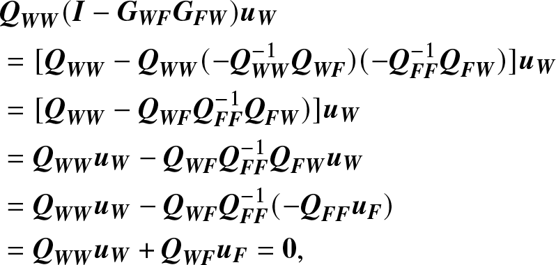 \begin{align*}
& {{\bf{Q}}_{{\bf{WW}}}}({\bf{I}} - {{\bf{G}}_{{\bf{WF}}}}{{\bf{G}}_{{\bf{FW}}}}){{\bf{u}}_{\bf{W}}}\\
& = [ {{\bf{Q}}_{{\bf{WW}}}} - {{\bf{Q}}_{{\bf{WW}}}}( - {\bf{Q}}_{{\bf{WW}}}^{- 1}{{\bf{Q}}_{{\bf{WF}}}})( - {\bf{Q}}_{{\bf{FF}}}^{- 1}{{\bf{Q}}_{{\bf{FW}}}})]{{\bf{u}}_{\bf{W}}} \\
& = [ {{\bf{Q}}_{{\bf{WW}}}} - {{\bf{Q}}_{{\bf{WF}}}}{\bf{Q}}_{{\bf{FF}}}^{- 1}{{\bf{Q}}_{{\bf{FW}}}})]{{\bf{u}}_{\bf{W}}} \\
& = {{\bf{Q}}_{{\bf{WW}}}}{{\bf{u}}_{\bf{W}}} - {{\bf{Q}}_{{\bf{WF}}}}{\bf{Q}}_{{\bf{FF}}}^{- 1}{{\bf{Q}}_{{\bf{FW}}}}{{\bf{u}}_{\bf{W}}} \\
& = {{\bf{Q}}_{{\bf{WW}}}}{{\bf{u}}_{\bf{W}}} - {{\bf{Q}}_{{\bf{WF}}}}{\bf{Q}}_{{\bf{FF}}}^{- 1}( - {{\bf{Q}}_{{\bf{FF}}}}{{\bf{u}}_{\bf{F}}}) \\
& = {{\bf{Q}}_{{\bf{WW}}}}{{\bf{u}}_{\bf{W}}} + {{\bf{Q}}_{{\bf{WF}}}}{{\bf{u}}_{\bf{F}}} = {\bf{0}},
\end{align*}
\begin{align*}
& {{\bf{Q}}_{{\bf{WW}}}}({\bf{I}} - {{\bf{G}}_{{\bf{WF}}}}{{\bf{G}}_{{\bf{FW}}}}){{\bf{u}}_{\bf{W}}}\\
& = [ {{\bf{Q}}_{{\bf{WW}}}} - {{\bf{Q}}_{{\bf{WW}}}}( - {\bf{Q}}_{{\bf{WW}}}^{- 1}{{\bf{Q}}_{{\bf{WF}}}})( - {\bf{Q}}_{{\bf{FF}}}^{- 1}{{\bf{Q}}_{{\bf{FW}}}})]{{\bf{u}}_{\bf{W}}} \\
& = [ {{\bf{Q}}_{{\bf{WW}}}} - {{\bf{Q}}_{{\bf{WF}}}}{\bf{Q}}_{{\bf{FF}}}^{- 1}{{\bf{Q}}_{{\bf{FW}}}})]{{\bf{u}}_{\bf{W}}} \\
& = {{\bf{Q}}_{{\bf{WW}}}}{{\bf{u}}_{\bf{W}}} - {{\bf{Q}}_{{\bf{WF}}}}{\bf{Q}}_{{\bf{FF}}}^{- 1}{{\bf{Q}}_{{\bf{FW}}}}{{\bf{u}}_{\bf{W}}} \\
& = {{\bf{Q}}_{{\bf{WW}}}}{{\bf{u}}_{\bf{W}}} - {{\bf{Q}}_{{\bf{WF}}}}{\bf{Q}}_{{\bf{FF}}}^{- 1}( - {{\bf{Q}}_{{\bf{FF}}}}{{\bf{u}}_{\bf{F}}}) \\
& = {{\bf{Q}}_{{\bf{WW}}}}{{\bf{u}}_{\bf{W}}} + {{\bf{Q}}_{{\bf{WF}}}}{{\bf{u}}_{\bf{F}}} = {\bf{0}},
\end{align*}that is, the sum of each row of matrix  ${{\bf{Q}}_{{\bf{WW}}}}({\bf{I}} - {{\bf{G}}_{{\bf{WF}}}}{{\bf{G}}_{{\bf{FW}}}})$ is zero, then it completes the proof.
Lemma 4.3. Let  $\{X(t),t \ge 0\} $ be a finite-state time-homogenous Markov process with state space ${\bf{S}} = \{1,2, \ldots ,n\} $, and its transition rate matrix be Q. If ${\bf{S}} = {\bf{W}} \cup {\bf{F}}$ and ${\bf{W}} \cap {\bf{F}} = \phi $ and ${\rm{Rank}}({\bf{Q}}) = n - 1$, then $\mathop {\lim }\limits_{s \downarrow 0} [s{{\bf{T}}_1}(s)]$ and $\mathop {\lim }\limits_{s \downarrow 0} [s{{\bf{T}}_2}(s)]$ are independent of the initial probability vectors ${{\bf{\alpha }}_0}$ and ${{\bf{\beta }}_1}$, respectively.
Proof. First we have
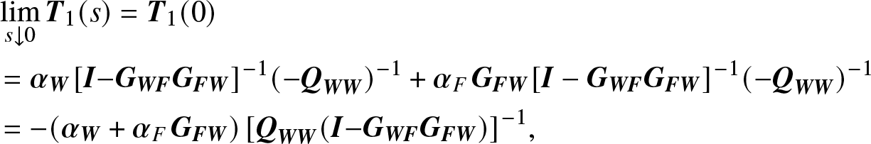 \begin{align*}
& \mathop {\lim }\limits_{s \downarrow 0} {{\bf{T}}_1}(s) = {{\bf{T}}_1}(0) \\
& = {{\bf{\alpha }}_{\bf{W}}} {[{\bf{I}}{\rm{- }}{{\bf{G}}_{{\bf{WF}}}}{{\bf{G}}_{{\bf{FW}}}}]^{- 1}}{( - {{\bf{Q}}_{{\bf{WW}}}})^{- 1}} + {{\bf{\alpha }}_F}{\kern 1pt} {{\bf{G}}_{{\bf{FW}}}}{[{\bf{I}} - {{\bf{G}}_{{\bf{WF}}}}{{\bf{G}}_{{\bf{FW}}}}]^{- 1}}{( - {{\bf{Q}}_{{\bf{WW}}}})^{- 1}} \\
& = - ({{\bf{\alpha }}_{\bf{W}}} + {{\bf{\alpha }}_F}{\kern 1pt} {{\bf{G}}_{{\bf{FW}}}}){\kern 1pt} {[{{\bf{Q}}_{{\bf{WW}}}}({\bf{I}}{\rm{- }}{{\bf{G}}_{{\bf{WF}}}}{{\bf{G}}_{{\bf{FW}}}})]^{- 1}},
\end{align*}
\begin{align*}
& \mathop {\lim }\limits_{s \downarrow 0} {{\bf{T}}_1}(s) = {{\bf{T}}_1}(0) \\
& = {{\bf{\alpha }}_{\bf{W}}} {[{\bf{I}}{\rm{- }}{{\bf{G}}_{{\bf{WF}}}}{{\bf{G}}_{{\bf{FW}}}}]^{- 1}}{( - {{\bf{Q}}_{{\bf{WW}}}})^{- 1}} + {{\bf{\alpha }}_F}{\kern 1pt} {{\bf{G}}_{{\bf{FW}}}}{[{\bf{I}} - {{\bf{G}}_{{\bf{WF}}}}{{\bf{G}}_{{\bf{FW}}}}]^{- 1}}{( - {{\bf{Q}}_{{\bf{WW}}}})^{- 1}} \\
& = - ({{\bf{\alpha }}_{\bf{W}}} + {{\bf{\alpha }}_F}{\kern 1pt} {{\bf{G}}_{{\bf{FW}}}}){\kern 1pt} {[{{\bf{Q}}_{{\bf{WW}}}}({\bf{I}}{\rm{- }}{{\bf{G}}_{{\bf{WF}}}}{{\bf{G}}_{{\bf{FW}}}})]^{- 1}},
\end{align*}and  $\mathop {\lim }\limits_{s \downarrow 0} {{\bf{T}}_2}(s) = - {\bf{\beta }}_1 {{\bf{G}}_{{\bf{FW}}}} {[{{\bf{Q}}_{{\bf{WW}}}}({\bf{I}}{\rm{- }}{{\bf{G}}_{{\bf{WF}}}}{{\bf{G}}_{{\bf{FW}}}})]^{- 1}}$. But from Lemma 4.2, we can know that both $\mathop {\lim }\limits_{s \downarrow 0} {{\bf{T}}_1}(s)$ and $\mathop {\lim }\limits_{s \downarrow 0} {{\bf{T}}_2}(s)$ do not exist. Thus, we cannot directly get the $\mathop {\lim }\limits_{s \downarrow 0} [s{{\bf{T}}_i}(s)]$ $(i = 1,2)$ by replacing s with zero.
Now we consider the inversed matrix  ${\bf{P}}(s)$ directly for a given transition rate matrix Q when ${\rm{Rank}}({\bf{Q}}) = n - 1$,
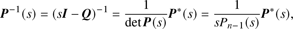 \begin{equation}
{{\bf{P}}^{- 1}}(s) = {(s{\bf{I}} - {\bf{Q}})^{- 1}} = {1 \over {\det {\bf{P}}(s)}}{{\bf{P}}^*}(s) = {1 \over {s{P_{n - 1}}(s)}}{{\bf{P}}^*}(s),
\end{equation}
\begin{equation}
{{\bf{P}}^{- 1}}(s) = {(s{\bf{I}} - {\bf{Q}})^{- 1}} = {1 \over {\det {\bf{P}}(s)}}{{\bf{P}}^*}(s) = {1 \over {s{P_{n - 1}}(s)}}{{\bf{P}}^*}(s),
\end{equation}where  ${P_{n - 1}}(s)$ is a polynomial of s such that ${P_{n - 1}}(0) \ne 0$, and the adjugate matrix ${{\bf{P}}^*}(s)$ given by
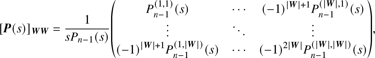
 \begin{equation*}
{{\bf{P}}^*}(s) = \left(
\begin{matrix}
{\det [{{\bf{P}}_{11}}(s)]} & {- \det [{{\bf{P}}_{21}}(s)]} & \cdots & {{{( - 1)}^{n + 1}}\det [{{\bf{P}}_{n1}}(s)]} \\
{- \det [{{\bf{P}}_{12}}(s)]} & {\det [{{\bf{P}}_{22}}(s)]} & \cdots & {{{( - 1)}^{n + 2}}\det [{{\bf{P}}_{n2}}(s)]} \\
\vdots & \vdots & \ddots & \vdots \\
{{{( - 1)}^{n + 1}}\det [{{\bf{P}}_{1n}}(s)]} & {{{( - 1)}^{n + 2}}\det [{{\bf{P}}_{2n}}(s)]} & \cdots & {\det [{{\bf{P}}_{nn}}(s)]}
\end{matrix}
\right).
\end{equation*}
\begin{equation*}
{{\bf{P}}^*}(s) = \left(
\begin{matrix}
{\det [{{\bf{P}}_{11}}(s)]} & {- \det [{{\bf{P}}_{21}}(s)]} & \cdots & {{{( - 1)}^{n + 1}}\det [{{\bf{P}}_{n1}}(s)]} \\
{- \det [{{\bf{P}}_{12}}(s)]} & {\det [{{\bf{P}}_{22}}(s)]} & \cdots & {{{( - 1)}^{n + 2}}\det [{{\bf{P}}_{n2}}(s)]} \\
\vdots & \vdots & \ddots & \vdots \\
{{{( - 1)}^{n + 1}}\det [{{\bf{P}}_{1n}}(s)]} & {{{( - 1)}^{n + 2}}\det [{{\bf{P}}_{2n}}(s)]} & \cdots & {\det [{{\bf{P}}_{nn}}(s)]}
\end{matrix}
\right).
\end{equation*} On the other hand, we have  ${{\bf{P}}_{ij}}(s) = s{\bf{I}} - {{\bf{Q}}_{ij}},{\rm{~}}i,j \in {\bf{S}},$ where ${{\bf{Q}}_{ij}}$ is a matrix obtained by deleting the ith row and jth column of Q. Obviously, we known that $\det[ {{\bf{P}}_{ij}}(s)]$ is a polynomial of s with degree n − 1. Let $\det [{{\bf{P}}_{ij}}(s)] = P_{n - 1}^{(i,j)}(s)$. Thus, we have
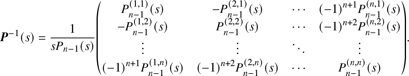 \begin{equation*}\bf P^{-1}(s)=\frac1{sP_{n-1}(s)}{\left(
\begin{matrix}
P_{n-1}^{(1,1)}(s)& -P_{n-1}^{(2,1)}(s)& \cdots & {(-1)}^{n+1}P_{n-1}^{(n,1)}(s)\\
-P_{n-1}^{(1,2)}(s)& P_{n-1}^{(2,2)}(s)& \cdots& {(-1)}^{n+2}P_{n-1}^{(n,2)}(s)\\
\vdots&\vdots&\ddots&\vdots\\
{(-1)}^{n+1}P_{n-1}^{(1,n)}(s)& {(-1)}^{n+2}P_{n-1}^{(2,n)}(s)& \cdots& P_{n-1}^{(n,n)}(s)\end{matrix}\right)}.\end{equation*}
\begin{equation*}\bf P^{-1}(s)=\frac1{sP_{n-1}(s)}{\left(
\begin{matrix}
P_{n-1}^{(1,1)}(s)& -P_{n-1}^{(2,1)}(s)& \cdots & {(-1)}^{n+1}P_{n-1}^{(n,1)}(s)\\
-P_{n-1}^{(1,2)}(s)& P_{n-1}^{(2,2)}(s)& \cdots& {(-1)}^{n+2}P_{n-1}^{(n,2)}(s)\\
\vdots&\vdots&\ddots&\vdots\\
{(-1)}^{n+1}P_{n-1}^{(1,n)}(s)& {(-1)}^{n+2}P_{n-1}^{(2,n)}(s)& \cdots& P_{n-1}^{(n,n)}(s)\end{matrix}\right)}.\end{equation*} Besides, we can prove that  ${( - 1)^{i + j}}\det [{{\bf{P}}_{ij}}(0)] = {( - 1)^{i + l}}\det [{{\bf{P}}_{il}}(0)]$ for any $i,j,l \in {\bf{S}}$. This is because, if we denote ${p_{ij}}(0) \equiv {p_{ij}},$ for any $i,j \in {\bf{S}},$ then it is clear that ${\bf{P}}(0) = {\left( {{p_{ij}}(0)} \right)_{n \times n}} = - {\bf{Q}}: = {\left( {{p_{ij}}} \right)_{n \times n}}$. Without loss of generality, it is assumed j < l, and then
 \begin{align*}&\operatorname{det}\lbrack{\bf P}_{ij}(0)\rbrack\\
&=\operatorname{det}\lbrack{\left(\begin{array}{@{\kern-0.1pt}cccccccccc@{\kern-0.1pt}}p_{11}& \cdots & p_{1(j-1)} & p_{1(j+1)} & \cdots & p_{1(l-1)} & p_{1l} & p_{1(l+1)} & \cdots & p_{1n}\\
\vdots & \ddots & \vdots & \vdots & \ddots & \vdots & \vdots & \vdots & \ddots & \vdots\\
p_{(i-1)1} & \cdots & p_{(i-1)(j-1)} & p_{(i-1)(j+1)} & \cdots & p_{(i-1)(l-1)} & p_{(i-1)l} & p_{(i-1)(l+1)} & \cdots & p_{(i-1)n}\\
p_{(i+1)1} & \cdots & p_{(i+1)(j-1)} & p_{(i+1)(j+1)} & \cdots & p_{(i+1)(l-1)} & p_{(i+1)l} & p_{(i+1)(l+1)} & \cdots & p_{(i+1)n}\\\vdots & \ddots & \vdots & \vdots & \ddots & \vdots & \vdots & \vdots & \ddots & \vdots\\
p_{n1} & \cdots & p_{n(j-1)} & p_{n(j+1)} & \cdots & p_{n(l-1)} & p_{nl} & p_{n(l+1)} & \cdots & p_{nn}\end{array}\right)}\rbrack\\
& =\operatorname{det}\lbrack{\left(\begin{array}{@{\kern-0.1pt}cccccccccc@{\kern-0.1pt}}p_{11} & \cdots & p_{1(j-1)} & p_{1(j+1)} & \cdots & p_{1(l-1)} &- p_{1j} & p_{1(l+1)} & \cdots & p_{1n}\\
\vdots & \ddots & \vdots & \vdots & \ddots & \vdots & \vdots & \vdots & \ddots & \vdots\\
p_{(i-1)1} & \cdots & p_{(i-1)(j-1)} & p_{(i-1)(j+1)} & \cdots & p_{(i-1)(l-1)} & -p_{(i-1)j} & p_{(i-1)(l+1)} & \cdots & p_{(i-1)n}\\
p_{(i+1)1} & \cdots & p_{(i+1)(j-1)} & p_{(i+1)(j+1)} & \cdots & p_{(i+1)(l-1)} & -p_{(i+1)j} & p_{(i+1)(l+1)} & \cdots & p_{(i+1)n}\\
\vdots & \ddots & \vdots & \vdots & \ddots & \vdots & \vdots & \vdots & \ddots & \vdots\\
p_{n1} & \cdots & p_{n(j-1)} & p_{n(j+1)} & \cdots & p_{n(l-1)} & -p_{nj} & p_{n(l+1)} & \cdots & p_{nn}\end{array}\right)}\rbrack.\end{align*}
\begin{align*}&\operatorname{det}\lbrack{\bf P}_{ij}(0)\rbrack\\
&=\operatorname{det}\lbrack{\left(\begin{array}{@{\kern-0.1pt}cccccccccc@{\kern-0.1pt}}p_{11}& \cdots & p_{1(j-1)} & p_{1(j+1)} & \cdots & p_{1(l-1)} & p_{1l} & p_{1(l+1)} & \cdots & p_{1n}\\
\vdots & \ddots & \vdots & \vdots & \ddots & \vdots & \vdots & \vdots & \ddots & \vdots\\
p_{(i-1)1} & \cdots & p_{(i-1)(j-1)} & p_{(i-1)(j+1)} & \cdots & p_{(i-1)(l-1)} & p_{(i-1)l} & p_{(i-1)(l+1)} & \cdots & p_{(i-1)n}\\
p_{(i+1)1} & \cdots & p_{(i+1)(j-1)} & p_{(i+1)(j+1)} & \cdots & p_{(i+1)(l-1)} & p_{(i+1)l} & p_{(i+1)(l+1)} & \cdots & p_{(i+1)n}\\\vdots & \ddots & \vdots & \vdots & \ddots & \vdots & \vdots & \vdots & \ddots & \vdots\\
p_{n1} & \cdots & p_{n(j-1)} & p_{n(j+1)} & \cdots & p_{n(l-1)} & p_{nl} & p_{n(l+1)} & \cdots & p_{nn}\end{array}\right)}\rbrack\\
& =\operatorname{det}\lbrack{\left(\begin{array}{@{\kern-0.1pt}cccccccccc@{\kern-0.1pt}}p_{11} & \cdots & p_{1(j-1)} & p_{1(j+1)} & \cdots & p_{1(l-1)} &- p_{1j} & p_{1(l+1)} & \cdots & p_{1n}\\
\vdots & \ddots & \vdots & \vdots & \ddots & \vdots & \vdots & \vdots & \ddots & \vdots\\
p_{(i-1)1} & \cdots & p_{(i-1)(j-1)} & p_{(i-1)(j+1)} & \cdots & p_{(i-1)(l-1)} & -p_{(i-1)j} & p_{(i-1)(l+1)} & \cdots & p_{(i-1)n}\\
p_{(i+1)1} & \cdots & p_{(i+1)(j-1)} & p_{(i+1)(j+1)} & \cdots & p_{(i+1)(l-1)} & -p_{(i+1)j} & p_{(i+1)(l+1)} & \cdots & p_{(i+1)n}\\
\vdots & \ddots & \vdots & \vdots & \ddots & \vdots & \vdots & \vdots & \ddots & \vdots\\
p_{n1} & \cdots & p_{n(j-1)} & p_{n(j+1)} & \cdots & p_{n(l-1)} & -p_{nj} & p_{n(l+1)} & \cdots & p_{nn}\end{array}\right)}\rbrack.\end{align*}On the other hand, we have
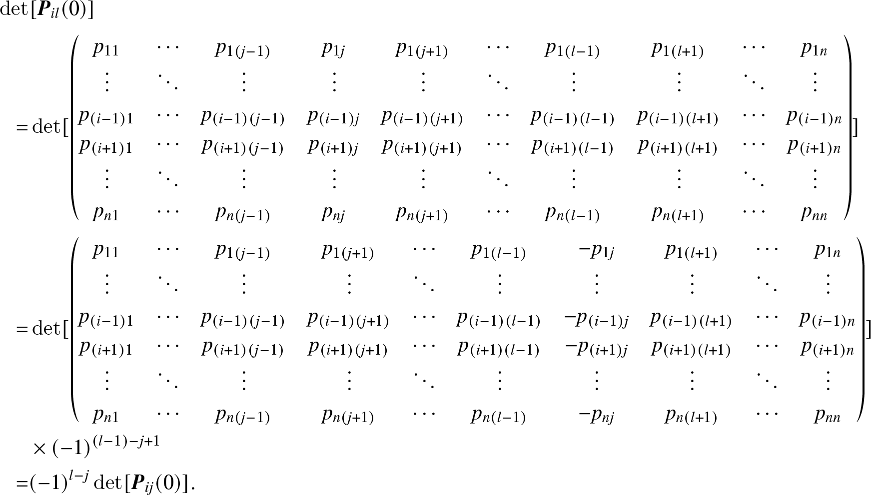 \begin{align*}\operatorname{det}&\lbrack{\bf P}_{il}(0)\rbrack\\=&\operatorname{det}\lbrack{\left(\begin{array}{@{\kern-0.1pt}cccccccccc@{\kern-0.1pt}}p_{11}&\cdots&p_{1(j-1)}&p_{1j}&p_{1(j+1)}&\cdots&p_{1(l-1)}&p_{1(l+1)}&\cdots&p_{1n}\\\vdots&\ddots&\vdots&\vdots&\vdots&\ddots&\vdots&\vdots&\ddots&\vdots\\p_{(i-1)1}&\cdots&p_{(i-1)(j-1)}&p_{(i-1)j}&p_{(i-1)(j+1)}&\cdots&p_{(i-1)(l-1)}&p_{(i-1)(l+1)}&\cdots&p_{(i-1)n}\\p_{(i+1)1}&\cdots&p_{(i+1)(j-1)}&p_{(i+1)j}&p_{(i+1)(j+1)}&\cdots&p_{(i+1)(l-1)}&p_{(i+1)(l+1)}&\cdots&p_{(i+1)n}\\\vdots&\ddots&\vdots&\vdots&\vdots&\ddots&\vdots&\vdots&\ddots&\vdots\\p_{n1}&\cdots&p_{n(j-1)}&p_{nj}&p_{n(j+1)}&\cdots&p_{n(l-1)}&p_{n(l+1)}&\cdots&p_{nn}\end{array}\right)}\rbrack\\=&\operatorname{det}\lbrack{\left(\begin{array}{@{\kern-0.1pt}cccccccccc@{\kern-0.1pt}}p_{11}&\cdots&p_{1(j-1)}&p_{1(j+1)}&\cdots&p_{1(l-1)}&-p_{1j}&p_{1(l+1)}&\cdots&p_{1n}\\\vdots&\ddots&\vdots&\vdots&\ddots&\vdots&\vdots&\vdots&\ddots&\vdots\\p_{(i-1)1}&\cdots&p_{(i-1)(j-1)}&p_{(i-1)(j+1)}&\cdots&p_{(i-1)(l-1)}&-p_{(i-1)j}&p_{(i-1)(l+1)}&\cdots&p_{(i-1)n}\\p_{(i+1)1}&\cdots&p_{(i+1)(j-1)}&p_{(i+1)(j+1)}&\cdots&p_{(i+1)(l-1)}&-p_{(i+1)j}&p_{(i+1)(l+1)}&\cdots&p_{(i+1)n}\\\vdots&\ddots&\vdots&\vdots&\ddots&\vdots&\vdots&\vdots&\ddots&\vdots\\p_{n1}&\cdots&p_{n(j-1)}&p_{n(j+1)}&\cdots&p_{n(l-1)}&-p_{nj}&p_{n(l+1)}&\cdots&p_{nn}\end{array}\right)}\rbrack\\&\times{(-1)^{(l-1)-j+1}}\\=&{(-1)^{l-j}}\operatorname{det}\lbrack{\bf P}_{ij}(0)\rbrack.\end{align*}
 Thus, we have proved that  $\det ({{\bf{P}}_{i1}}(0)) = -\det ({{\bf{P}}_{i2}}(0)) = \cdots = {( - 1)^{n - 1}}\det ({{\bf{P}}_{in}}(0))$, for any $i \in {\bf{S}}$, which implies that matrix ${{\bf{P}}^*}(0)$ has the same row, that is, each column in matrix ${{\bf{P}}^*}(0)$ consists in the same value.
Furthermore, based on the result of inversion of partitioned matrix presented in Section 2, we have
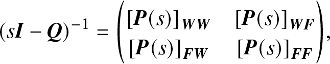 \begin{equation*}{(s\bf I-\bf Q)^{-1}}={\left(\begin{array}{@{\kern-0.1pt}cc@{\kern-0.1pt}}{\lbrack\bf P(s)\rbrack}_{\bf W\bf W}&{\lbrack\bf P(s)\rbrack}_{\bf W\bf F}\\{\lbrack\bf P(s)\rbrack}_{\bf F\bf W}&{\lbrack\bf P(s)\rbrack}_{\bf F\bf F}\end{array}\right)},\end{equation*}
where  ${[{\bf{P}}(s)]_{{\bf{WW}}}} = {[{\bf{I}} - {\bf{G}}_{{\bf{WF}}}^*(s){\bf{G}}_{{\bf{FW}}}^*(s)]^{- 1}}{\bf{P}}_{{\bf{WW}}}^*(s),$ and
 \begin{equation*}{[{\bf{P}}(s)]_{{\bf{FW}}}} = {\bf{G}}_{{\bf{FW}}}^*(s){[{\bf{I}} - {\bf{G}}_{{\bf{WF}}}^*(s){\bf{G}}_{{\bf{FW}}}^*(s)]^{- 1}}{\bf{P}}_{{\bf{WW}}}^*(s).\end{equation*}
On the other hand, from Eq. (4.4), we have
 \begin{equation*}{\lbrack\bf P(s)\rbrack_{\bf W\bf W}}=\frac1{sP_{n-1}(s)}{\left(\begin{array}{@{\kern-0.1pt}ccc@{\kern-0.1pt}}P_{n-1}^{(1,1)}(s)&\cdots&{(-1)}^{\vert\bf W\vert+1}P_{n-1}^{(\vert\bf W\vert,1)}(s)\\\vdots&\ddots&\vdots\\{(-1)}^{\vert\bf W\vert+1}P_{n-1}^{(1,\vert\bf W\vert)}(s)&\cdots&{(-1)}^{2\vert\bf W\vert}P_{n-1}^{(\vert\bf W\vert,\vert\bf W\vert)}(s)\end{array}\right)},\end{equation*}
 \begin{equation*}{\lbrack\bf P(s)\rbrack_{\bf F\bf W}}=\frac1{sP_{n-1}(s)}{\left(\begin{array}{@{\kern-0.1pt}ccc@{\kern-0.1pt}}{(-1)}^{\vert\bf W\vert+2}P_{n-1}^{(1,\vert\bf W\vert+1)}(s)&\cdots&{(-1)}^{2\vert\bf W\vert+1}P_{n-1}^{(\vert\bf W\vert,\vert\bf W\vert+1)}(s)\\\vdots&\ddots&\vdots\\{(-1)}^{\vert\bf W\vert+\vert\bf F\vert+1}P_{n-1}^{(1,\vert\bf W\vert+\vert\bf F\vert)}(s)&\cdots&{(-1)}^{2\vert\bf W\vert+\vert\bf F\vert}P_{n-1}^{(\vert\bf W\vert,\vert\bf W\vert+\vert\bf F\vert)}(s)\end{array}\right)}.\end{equation*}
Thus, we have
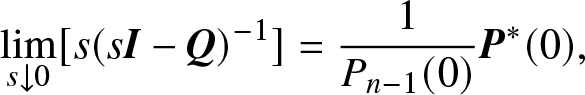 \begin{equation}
\mathop {\lim }\limits_{s \downarrow 0} [s{(s{\bf{I}} - {\bf{Q}})^{- 1}}] = {1 \over {{P_{n - 1}}(0)}}{{\bf{P}}^*}(0),
\end{equation}
\begin{equation}
\mathop {\lim }\limits_{s \downarrow 0} [s{(s{\bf{I}} - {\bf{Q}})^{- 1}}] = {1 \over {{P_{n - 1}}(0)}}{{\bf{P}}^*}(0),
\end{equation}with the same row, that is,
 \begin{equation*}
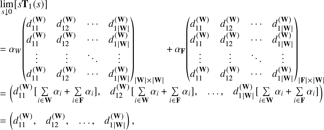
\begin{array}{*{20}{@{\kern-0.1pt}llll@{\kern-0.1pt}}}
{\mathop {\lim }\limits_{s \downarrow 0} [s{{\mathbf{T}}_1}(s)]} \\
{ = {{\mathbf{\alpha }}_W}{{\left( {\begin{array}{*{20}{@{\kern-0.1pt}cccc@{\kern-0.1pt}}}
{d_{11}^{({\mathbf{W}})}}&{d_{12}^{({\mathbf{W}})}}& \cdots &{d_{1|{\mathbf{W}}|}^{({\mathbf{W}})}} \\
{d_{11}^{({\mathbf{W}})}}&{d_{12}^{({\mathbf{W}})}}& \cdots &{d_{1|{\mathbf{W}}|}^{({\mathbf{W}})}} \\
\vdots & \vdots & \ddots & \vdots \\
{d_{11}^{({\mathbf{W}})}}&{d_{12}^{({\mathbf{W}})}}& \cdots &{d_{1|{\mathbf{W}}|}^{({\mathbf{W}})}}
\end{array}} \right)}_{|{\mathbf{W}}| \times |{\mathbf{W}}|}} + {{\mathbf{\alpha }}_{\mathbf{F}}}{{\left( {\begin{array}{*{20}{@{\kern-0.1pt}cccc@{\kern-0.1pt}}}
{d_{11}^{({\mathbf{W}})}}&{d_{12}^{({\mathbf{W}})}}& \cdots &{d_{1|{\mathbf{W}}|}^{({\mathbf{W}})}} \\
{d_{11}^{({\mathbf{W}})}}&{d_{12}^{({\mathbf{W}})}}& \cdots &{d_{1|{\mathbf{W}}|}^{({\mathbf{W}})}} \\
\vdots & \vdots & \ddots & \vdots \\
{d_{11}^{({\mathbf{W}})}}&{d_{12}^{({\mathbf{W}})}}& \cdots &{d_{1|{\mathbf{W}}|}^{({\mathbf{W}})}}
\end{array}} \right)}_{|{\mathbf{F}}| \times |{\mathbf{W}}|}}} \\ [18pt]
{ = \left( {\begin{array}{*{20}{@{\kern-0.1pt}cccc@{\kern-0.1pt}}}
{d_{11}^{({\mathbf{W}})}[\sum\limits_{i \in {\mathbf{W}}} {{\alpha _i}} + \sum\limits_{i \in {\mathbf{F}}} {{\alpha _i}],} }&{d_{12}^{({\mathbf{W}})}[\sum\limits_{i \in {\mathbf{W}}} {{\alpha _i}} + \sum\limits_{i \in {\mathbf{F}}} {{\alpha _i}],} }&{ \ldots ,}&{d_{1|{\mathbf{W}}|}^{({\mathbf{W}})}[\sum\limits_{i \in {\mathbf{W}}} {{\alpha _i}} + \sum\limits_{i \in {\mathbf{F}}} {{\alpha _i}]} }
\end{array}} \right)} \\ [12pt]
{ = \left( {\begin{array}{*{20}{@{\kern-0.1pt}cccc@{\kern-0.1pt}}}
{d_{11}^{({\mathbf{W}})},}&{d_{12}^{({\mathbf{W}})},}&{ \ldots ,}&{d_{1|{\mathbf{W}}|}^{({\mathbf{W}})}}
\end{array}} \right),}
\end{array}
\end{equation*}
\begin{equation*}
\begin{array}{*{20}{@{\kern-0.1pt}llll@{\kern-0.1pt}}}
{\mathop {\lim }\limits_{s \downarrow 0} [s{{\mathbf{T}}_1}(s)]} \\
{ = {{\mathbf{\alpha }}_W}{{\left( {\begin{array}{*{20}{@{\kern-0.1pt}cccc@{\kern-0.1pt}}}
{d_{11}^{({\mathbf{W}})}}&{d_{12}^{({\mathbf{W}})}}& \cdots &{d_{1|{\mathbf{W}}|}^{({\mathbf{W}})}} \\
{d_{11}^{({\mathbf{W}})}}&{d_{12}^{({\mathbf{W}})}}& \cdots &{d_{1|{\mathbf{W}}|}^{({\mathbf{W}})}} \\
\vdots & \vdots & \ddots & \vdots \\
{d_{11}^{({\mathbf{W}})}}&{d_{12}^{({\mathbf{W}})}}& \cdots &{d_{1|{\mathbf{W}}|}^{({\mathbf{W}})}}
\end{array}} \right)}_{|{\mathbf{W}}| \times |{\mathbf{W}}|}} + {{\mathbf{\alpha }}_{\mathbf{F}}}{{\left( {\begin{array}{*{20}{@{\kern-0.1pt}cccc@{\kern-0.1pt}}}
{d_{11}^{({\mathbf{W}})}}&{d_{12}^{({\mathbf{W}})}}& \cdots &{d_{1|{\mathbf{W}}|}^{({\mathbf{W}})}} \\
{d_{11}^{({\mathbf{W}})}}&{d_{12}^{({\mathbf{W}})}}& \cdots &{d_{1|{\mathbf{W}}|}^{({\mathbf{W}})}} \\
\vdots & \vdots & \ddots & \vdots \\
{d_{11}^{({\mathbf{W}})}}&{d_{12}^{({\mathbf{W}})}}& \cdots &{d_{1|{\mathbf{W}}|}^{({\mathbf{W}})}}
\end{array}} \right)}_{|{\mathbf{F}}| \times |{\mathbf{W}}|}}} \\ [18pt]
{ = \left( {\begin{array}{*{20}{@{\kern-0.1pt}cccc@{\kern-0.1pt}}}
{d_{11}^{({\mathbf{W}})}[\sum\limits_{i \in {\mathbf{W}}} {{\alpha _i}} + \sum\limits_{i \in {\mathbf{F}}} {{\alpha _i}],} }&{d_{12}^{({\mathbf{W}})}[\sum\limits_{i \in {\mathbf{W}}} {{\alpha _i}} + \sum\limits_{i \in {\mathbf{F}}} {{\alpha _i}],} }&{ \ldots ,}&{d_{1|{\mathbf{W}}|}^{({\mathbf{W}})}[\sum\limits_{i \in {\mathbf{W}}} {{\alpha _i}} + \sum\limits_{i \in {\mathbf{F}}} {{\alpha _i}]} }
\end{array}} \right)} \\ [12pt]
{ = \left( {\begin{array}{*{20}{@{\kern-0.1pt}cccc@{\kern-0.1pt}}}
{d_{11}^{({\mathbf{W}})},}&{d_{12}^{({\mathbf{W}})},}&{ \ldots ,}&{d_{1|{\mathbf{W}}|}^{({\mathbf{W}})}}
\end{array}} \right),}
\end{array}
\end{equation*}where  $d_{ij}^{({\bf{W}})} = {( - 1)^{i + j}}{{P_{n - 1}^{(j,i)}(0)} \over {{P_{n - 1}}(0)}}$, $i,j \in {\bf{S}}$. Thus, we can have that $\mathop {\lim }\limits_{s \downarrow 0} [s{{\bf{T}}_1}(s)]$ does not depend on the initial probability vector ${\bf{\alpha }_0} = ({{\bf{\alpha }}_{\bf{W}}},{{\bf{\alpha }}_{\bf{F}}}).$
Similarly, we have that  $\mathop {\lim }\limits_{s \downarrow 0} [s{{\bf{T}}_2}(s)]$ does not depend on ${{\bf{\beta }}_1}$. Thus, it completes the proof.
Theorem 4.1. Let  $\{X(t),t \ge 0\} $ be a finite-state time-homogenous Markov process with state space ${\bf{S}} = \{1,2, \ldots ,n\} $, and its transition rate matrix be Q. If ${\bf{S}} = {\bf{W}} \cup {\bf{F}}$, ${\bf{W}} \cap {\bf{F}} = \phi $, and ${\rm{Rank}}({\bf{Q}}) = n - 1$, then the steady-state availability $\mathop {\lim }\limits_{t \to \infty } A(t)$, the steady-state interval availability $\mathop {\lim }\limits_{t \to \infty } A([t,t + a])$, the steady-state transition probability between two subsets $\mathop {\lim }\limits_{t \to \infty } {p_{{{\bf{S}}_1}{{\bf{S}}_2}}}(t)$, and the steady-state probability staying in a given subset $\mathop {\lim }\limits_{t \to \infty } {p_{{{\bf{S}}_0}}}(t)$, given in matrix expressions by using aggregated stochastic process theory, are independent of the initial probability vectors ${{\bf{\alpha }}_0}$ and ${{\bf{\beta }}_1}$, respectively.
Proof. Based on the results given in Lemma 4.3, it is clear to know that Theorem 4.1 holds.
Note: For Theorem 4.1, it seems we can understand that the  $\mathop {\lim }\limits_{t \to \infty } A(t)$, $\mathop {\lim }\limits_{t \to \infty } A([t,t + a])$, $\mathop {\lim }\limits_{t \to \infty } {p_{{{\mathbf{S}}_1}{{\mathbf{S}}_2}}}(t)$, and $\mathop {\lim }\limits_{t \to \infty } {p_{{{\bf{S}}_0}}}(t)$ are independent of the initial probability condition for aggregated Markov processes when ${\rm{Rank}}({\bf{Q}}) = n - 1$, namely there is at most one absorbing state for the underlying Markov process, see Examples 5.1 and 5.2, for example. In fact, the limiting behaviors of a finite irreducible aggregated Markov process are independent of the initial probability condition, so that it is also true under condition ${\rm{Rank}}({\bf{Q}}) = n - 1$.
5. Numerical examples and discussion
In this section, some examples will be presented by using the direct computation way to illustrate the independence of initial probability vectors for direct limits such as steady-state interval and point availabilities, steady-state transition probability between two subsets, and steady-state probability staying in a given subset, which have all been proved and expressed in Theorem 4.1.
Example 5.1. (Case that  ${\rm{Rank}}({\bf{Q}}) = n - 1$ and all states communicate.) Suppose that n = 4, all states in ${\bf{S}} = \{1,2,3,4\} $ communicate with each other, with ${\bf{W}} = \{1,2,3\} ,{\bf{F}} = \{4\} $ and
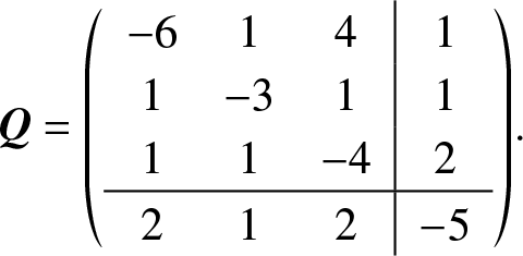 \begin{equation*}\bf Q={\left(\begin{array}{ccc|c}-6&1&4&1\\1&-3&1&1\\1&1&-4&2\\\hline2&1&2&-5\end{array}\right)}.\end{equation*}
 The transition diagram of  $\{X(t),t \ge 0\} $ is shown in Figure 1.

Figure 1. The transition diagram for Example 5.1.
We have  ${\rm{Rank}}({\bf{Q}}) = 3$, and
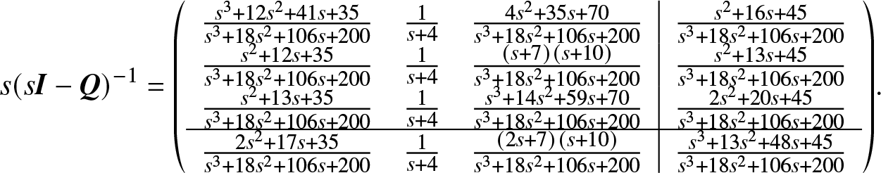 \begin{equation*}s{(s\bf I-\bf Q)^{-1}}={\left(\begin{array}{ccc|c}\frac{s^3+12s^2+41s+35}{s^3+18s^2+106s+200}&\frac1{s+4}&\frac{4s^2+35s+70}{s^3+18s^2+106s+200}&\frac{s^2+16s+45}{s^3+18s^2+106s+200}\\\frac{s^2+12s+35}{s^3+18s^2+106s+200}&\frac1{s+4}&\frac{(s+7)(s+10)}{s^3+18s^2+106s+200}&\frac{s^2+13s+45}{s^3+18s^2+106s+200}\\\frac{s^2+13s+35}{s^3+18s^2+106s+200}&\frac1{s+4}&\frac{s^3+14s^2+59s+70}{s^3+18s^2+106s+200}&\frac{2s^2+20s+45}{s^3+18s^2+106s+200}\\\hline\frac{2s^2+17s+35}{s^3+18s^2+106s+200}&\frac1{s+4}&\frac{(2s+7)(s+10)}{s^3+18s^2+106s+200}&\frac{s^3+13s^2+48s+45}{s^3+18s^2+106s+200}\end{array}\right)}.\end{equation*}
Taking the limit, we have
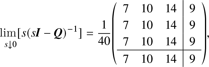 \begin{equation*}\underset{s\downarrow 0}{\operatorname{lim}\lbrack}{}s{(s\bf I-\bf Q)^{-1}}\rbrack=\frac1{40}{\left(\begin{array}{ccc|c}7&10&14&9\\7&10&14&9\\7&10&14&9\\\hline7&10&14&9\end{array}\right)},\end{equation*}
which shows that the matrixes  $\mathop {\lim }\limits_{s \downarrow 0} [s{{\bf{T}}_1}(s)] ={1 \over {40}} (7, 10,14)$ and $\mathop {\lim }\limits_{s \downarrow 0} [s{{\bf{T}}_2}(s)]={1 \over {40}} (7, 10,14)$ possess the same row; thus, the related steady-state indexes do not depend on the initial probability vector.
Example 5.2. (Case that  ${\rm{Rank}}({\bf{Q}}) = n - 1$ but not all states communicate with each other.) Suppose that n = 4, three states in ${\bf{S}} = \{1,2,3,4\} $ communicate with each other, but state 4 does not communicate with states 1, 2, and 3, with ${\bf{W}} = \{1,2,3\} ,{\bf{F}} = \{4\} $ and,
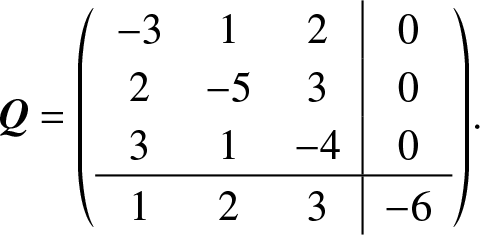 \begin{equation*}\bf Q={\left(\begin{array}{ccc|c}-3&1&2&0\\2&-5&3&0\\3&1&-4&0\\\hline1&2&3&-6\end{array}\right)}.\end{equation*}
 The transition diagram of  $\{X(t),t \ge 0\} $ is shown in Figure 2.

Figure 2. The transition diagram for Example 5.2.
We have  ${\rm{Rank}}({\bf{Q}}) = 3$, and
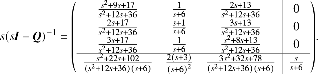 \begin{equation*}s{(s\bf I-\bf Q)^{-1}}={\left(\begin{array}{ccc|c}\frac{s^2+9s+17}{s^2+12s+36}&\frac1{s+6}&\frac{2s+13}{s^2+12s+36}&0\\\frac{2s+17}{s^2+12s+36}&\frac{s+1}{s+6}&\frac{3s+13}{s^2+12s+36}&0\\\frac{3s+17}{s^2+12s+36}&\frac1{s+6}&\frac{s^2+8s+13}{s^2+12s+36}&0\\\hline\frac{s^2+22s+102}{(s^2+12s+36)(s+6)}&\frac{2(s+3)}{{(s+6)}^2}&\frac{3s^2+32s+78}{(s^2+12s+36)(s+6)}&\frac s{s+6}\end{array}\right)}.\end{equation*}
Taking the limit, we have
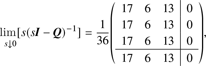 \begin{equation*}\underset{s\downarrow 0}{\operatorname{lim}\lbrack}{}s{(s\bf I-\bf Q)^{-1}}\rbrack=\frac1{36}{\left(\begin{array}{ccc|c}17&6&13&0\\17&6&13&0\\17&6&13&0\\\hline17&6&13&0\end{array}\right)},\end{equation*}
which shows that the matrixes  $\mathop {\lim }\limits_{s \downarrow 0} [s{{\bf{T}}_1}(s)] ={1 \over {36}} (17, 6,13)$ and $\mathop {\lim }\limits_{s \downarrow 0} [s{{\bf{T}}_2}(s)]={1 \over {36}} (17, 6,13)$ possess the same row; thus, the related steady-state indexes do not depend on the initial probability vector, although all states do not communicate anymore.
Example 5.3. (Case that  ${\rm{Rank}}({\bf{Q}}) = n - 2$, some states communicate and some not.) Suppose that n = 6, the state space ${\bf{S}} = \{1,2,3,4,5,6\} $, with ${\bf{W}} = \{1,2,3\} ,{}{\bf{F}} = \{4,5,6\}$ and
 \begin{equation*}\bf Q={\left(\begin{array}{ccc|ccc}-2&2&0&0&0&0\\1&-1&0&0&0&0\\1&2&-8&1&1&3\\\hline2&3&1&-10&3&1\\0&0&0&0&-2&2\\0&0&0&0&1&-1\end{array}\right)}.\end{equation*}
 Denote  ${\bf{S}} = {{\bf{S}}_1} \cup {{\bf{S}}_2} \cup {{\bf{S}}_3}$ with ${{\bf{S}}_1} = \{1,2\} $, ${{\bf{S}}_2} = \{3,4\}$, $ {{\bf{S}}_3} = \{5,6\} $. The states in ${{\bf{S}}_i}$ $ (i = 1,2,3)$ communicate with each other, and ${{\bf{S}}_2} \to {{\bf{S}}_1}, $ ${{\bf{S}}_1}\nrightarrow{{\bf{S}}_2}$ and ${{\bf{S}}_2} \to {{\bf{S}}_3},$ $ {{\bf{S}}_3}\nrightarrow{{\bf{S}}_2}$, that is, some states communicate each other, but some states do not. The transition diagram of $\{X(t),t \ge 0\} $ is shown in Figure 3.

Figure 3. The transition diagram for Example 5.3.
We have  ${\rm{Rank}}({\bf{Q}}) = 4$, and
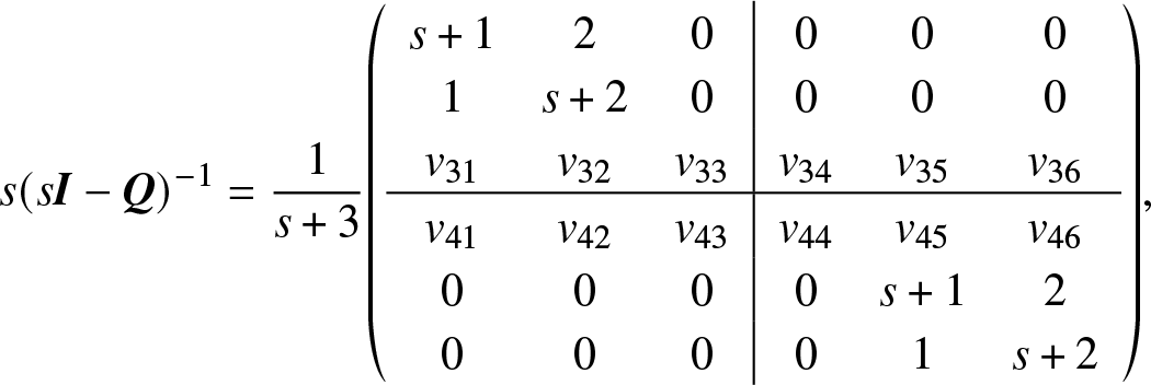 \begin{equation*}s{(s\bf I-\bf Q)^{-1}}=\frac1{s+3}{\left(\begin{array}{ccc|ccc}s+1&2&0&0&0&0\\1&s+2&0&0&0&0\\v_{31}&v_{32}&v_{33}&v_{34}&v_{35}&v_{36}\\\hline v_{41}&v_{42}&v_{43}&v_{44}&v_{45}&v_{46}\\0&0&0&0&s+1&2\\0&0&0&0&1&s+2\end{array}\right)},\end{equation*}
where
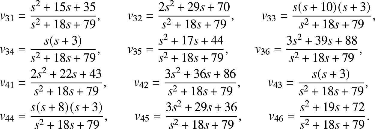 \begin{align*}
&{v_{31}} = {{{s^2} + 15s + 35} \over {{s^2} + 18s + 79}},\qquad {v_{32}} = {{2{s^2} + 29s + 70} \over {{s^2} + 18s + 79}},\qquad{v_{33}} = {{s(s+10)(s + 3)} \over {{s^2} + 18s + 79}},\\
&{v_{34}} = {{s(s + 3)} \over {{s^2} + 18s + 79}},\qquad{v_{35}} = {{{s^2} + 17s + 44} \over {{s^2} + 18s + 79}},\qquad{v_{36}} = {{3{s^2} + 39s + 88} \over {{s^2} + 18s + 79}},\\
&{v_{41}} = {{2{s^2} + 22s + 43} \over {{s^2} + 18s + 79}},\qquad{v_{42}} = {{3{s^2} + 36s + 86} \over {{s^2} + 18s + 79}},\qquad{v_{43}} = {{s(s + 3)} \over {{s^2} + 18s + 79}},\\
&{v_{44}} = {{s(s + 8)(s + 3)} \over {{s^2} + 18s + 79}},\qquad{v_{45}} = {{3{s^2} + 29s + 36} \over {{s^2} + 18s + 79}},\qquad{v_{46}} = {{{s^2} + 19s + 72} \over {{s^2} + 18s + 79}}.
\end{align*}
\begin{align*}
&{v_{31}} = {{{s^2} + 15s + 35} \over {{s^2} + 18s + 79}},\qquad {v_{32}} = {{2{s^2} + 29s + 70} \over {{s^2} + 18s + 79}},\qquad{v_{33}} = {{s(s+10)(s + 3)} \over {{s^2} + 18s + 79}},\\
&{v_{34}} = {{s(s + 3)} \over {{s^2} + 18s + 79}},\qquad{v_{35}} = {{{s^2} + 17s + 44} \over {{s^2} + 18s + 79}},\qquad{v_{36}} = {{3{s^2} + 39s + 88} \over {{s^2} + 18s + 79}},\\
&{v_{41}} = {{2{s^2} + 22s + 43} \over {{s^2} + 18s + 79}},\qquad{v_{42}} = {{3{s^2} + 36s + 86} \over {{s^2} + 18s + 79}},\qquad{v_{43}} = {{s(s + 3)} \over {{s^2} + 18s + 79}},\\
&{v_{44}} = {{s(s + 8)(s + 3)} \over {{s^2} + 18s + 79}},\qquad{v_{45}} = {{3{s^2} + 29s + 36} \over {{s^2} + 18s + 79}},\qquad{v_{46}} = {{{s^2} + 19s + 72} \over {{s^2} + 18s + 79}}.
\end{align*}Taking the limit, we have
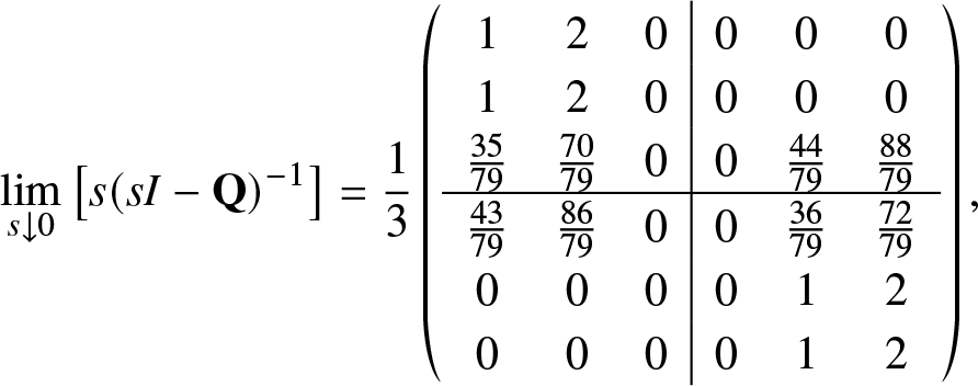 \begin{equation*}\mathop {\lim }\limits_{s \downarrow 0} \left[ {s{{\left( {s{\bf{\it{I}}} - {\mathbf{Q}}} \right)}^{ - 1}}} \right] = \frac{1}{3}\left( {\begin{array}{*{20}{ccc|ccc}}
1&2&0&0&0&0 \\
1&2&0&0&0&0 \\
{\frac{{35}}{{79}}}&{\frac{{70}}{{79}}}&0&0&{\frac{{44}}{{79}}}&{\frac{{88}}{{79}}} \\ \hline
{\frac{{43}}{{79}}}&{\frac{{86}}{{79}}}&0&0&{\frac{{36}}{{79}}}&{\frac{{72}}{{79}}} \\
0&0&0&0&1&2 \\
0&0&0&0&1&2
\end{array}} \right),\end{equation*}
\begin{equation*}\mathop {\lim }\limits_{s \downarrow 0} \left[ {s{{\left( {s{\bf{\it{I}}} - {\mathbf{Q}}} \right)}^{ - 1}}} \right] = \frac{1}{3}\left( {\begin{array}{*{20}{ccc|ccc}}
1&2&0&0&0&0 \\
1&2&0&0&0&0 \\
{\frac{{35}}{{79}}}&{\frac{{70}}{{79}}}&0&0&{\frac{{44}}{{79}}}&{\frac{{88}}{{79}}} \\ \hline
{\frac{{43}}{{79}}}&{\frac{{86}}{{79}}}&0&0&{\frac{{36}}{{79}}}&{\frac{{72}}{{79}}} \\
0&0&0&0&1&2 \\
0&0&0&0&1&2
\end{array}} \right),\end{equation*}which tells us that when  ${\rm{Rank}}({\bf{Q}}) \le n - 2$, the situation becomes complicated, which is our future research work.
In fact, from the knowledge of common finite irreducible Markov processes, we also have that the initial conditions do not affect the steady-state measures, regardless of the rank of transition rate matrix. Because, in general, for a finite state space of Markov process  $\{X(t),t \ge 0\} $, we have $\mathop {\lim }\limits_{t \to \infty } {P_{ij}}(t) = \mathop {\lim }\limits_{t \to \infty } P\{X(t) = j|X(0) = i\} = {\pi _j}$ and $\mathop {\lim }\limits_{t \to \infty } {P_i}(t) = \mathop {\lim }\limits_{t \to \infty } P\{X(t) = i\} = {\pi _i}$, both do not depend on the initial conditions of the underlying Markov process.
For aggregated Markov processes, if the steady-state measures are expressed by the Laplace transforms, it is not easy to known this result holds or not in terms of these Laplace transform formulas. In the previous contents, we prove it under the case of  ${\rm{Rank}}({\bf{Q}}) = n - 1$, while for the other cases that ${\rm{Rank}}({\bf{Q}}) \le n - 2$, it is sure that the conclusion holds too, but it seems to be complicated to prove it. Here a numerical example is presented for the case of ${\rm{Rank}}({\bf{Q}}) = n - 2$ in which the effects of the initial probability vector on the steady-state measures can be studied more deeply.
Example 5.3 also seems to provide a way to generate a transition rate matrix with  ${\rm{Rank}}({\bf{Q}}) = n - k, $ $k \in \{1,2, \ldots ,n - 1\} $, and gives some guidance to understand how the initial state probability vector affects the steady-state measures. Because, for example, the steady state probabilities staying at subsets ${{\bf{S}}_1}$ and ${{\bf{S}}_2}$ are $\mathop {\lim }\limits_{t \to \infty } {p_{{{\bf{S}}_1}}}(t) ={{\alpha}_1}+{{\alpha}_2}+{35\over {79}}{{\alpha}_3}+{43\over {79}}{{\alpha}_4}$ and $\mathop {\lim }\limits_{t \to \infty } {p_{{{\bf{S}}_3}}}(t) ={44\over {79}}{{\alpha}_3}+{36\over {79}}{{\alpha}_4}+{{\alpha}_5}+{{\alpha}_6}$. It is obvious to know that the steady-state probabilities depend on the initial probability vector ${{\bf{\alpha}}_0}=({{\alpha}_1},{{\alpha}_2},\ldots,{{\alpha}_6})$ through ${{\alpha}_1}+{{\alpha}_2}$ and ${{\alpha}_5}+{{\alpha}_6}$, respectively, instead of individual ${{\alpha}_1}$, ${{\alpha}_2}$ and ${{\alpha}_5},{{\alpha}_6}$.
6. Conclusion
In the paper, under the condition that  ${\rm{Rank}}({\bf{Q}}) = n - 1$, we directly prove that four limiting measures expressed by the Laplace transforms derived by using aggregated Markov processes do not depend on the initial state, which are well-known in common Markov processes. The condition ${\rm{Rank}}({\bf{Q}}) = n - 1$, which is more extensive than the case of time reversibility in ion channel modeling, includes the case that all states communicate with each other. Our work implies that (1) four limiting measures do not depend on the initial probability vector ${{\bf{\alpha }}_0}$, which is a well-known result in Markov repairable systems in terms of properties of Markov processes, but now this is a direct way to prove this result in aggregated Markov processes; (2) this proof can bridge a gap between the common knowledge in Markov processes and aggregated stochastic processes for the case of steady-state situation; (3) similar problems can be discussed, which are via a direct way based on the results in aggregated stochastic processes; (4) the initial probability vector ${{\bf{\alpha }}_0}$ appears in the formulas, but these limited results do not depend on this initial vector, which is an extension of one-dimensional case in which the initial value may disappear via the division of the same value in the formulas.
The possible future research work may include the study of similar problems under the cases of aggregated Semi-Markov processes, of  ${\rm{Rank}}({\bf{Q}}) \le n - 2$, and of time omission problems, and so on. We believe that our work can solid the theory and applications of aggregated Markov processes on the related limiting measures, especially in reliability field.
Acknowledgments
This work is supported by the National Natural Science Foundation of China under grants 72271134 and 71871021. We sincerely thank the Associate Editor and two anonymous referees for their valuable comments and suggestions.
Competing interests
There were no competing interests to declare which arose during the preparation or publication process of this article.


 Open access