


1. Introduction
Stellar luminosity varies slowly in the long-term evolution, but some stars exhibit noticeable luminosity changes on the short timescale (compared to the evolutionary timescale). These stars are called variable stars. Depending on the causes of variations, they are classified into intrinsic and extrinsic variables (Eyer & Mowlavi Reference Eyer and Mowlavi2008). Among them, the periodic variables display regular or semi-regular luminosity changes, and their periods are usually correlated with the physical or geometric properties of variables. The mass, luminosity, radius, and age of variables can be inferred from their periods using empirical relations (Chen et al. Reference Chen, Wang, Deng, de Grijs and Yang2018). Some variables, such as Cepheid stars and RR Lyrae stars, can serve as standard candles for distance measurement (Alloin & Gieren Reference Alloin and Gieren2003). Moreover, as tracers, they reveal the structure, chemical, and dynamical evolution of the Galaxy, as well as the substructure of the halo (Zhang, Zhang, & Zhao Reference Zhang, Zhang and Zhao2018; Koposov et al. Reference Koposov2019; Price-Whelan et al. Reference Price-Whelan2019; Prudil et al. Reference Prudil, Dékány, Grebel and Kunder2020). Therefore, periodic variables are not only crucial for studying the structure of galaxies but also can be used to constrain the stellar evolution model.
The development of large-scale sky survey projects, such as the Wide-field Infrared Survey Explorer (WISE; Wright et al. Reference Wright2010), Kepler (Koch et al. Reference Koch2010), and Catalina Real-Time Transient Survey (CRTS; Drake et al. Reference Drake2017), has enabled repeated observations of large areas of the sky every few nights. With the accumulation of abundant light curve data, the study of time-domain astronomy has become imperative. Time-domain astronomy is now entering a golden age, which spans across electromagnetic wavelengths from radio to gamma-rays (Graham et al. Reference Graham, Drake, Djorgovski, Mahabal and Donalek2017). In this new era of data explosion, it is impractical to classify variable stars by visual inspection alone. Therefore, it is essential to achieve automatic classification of massive variable stars and assign the unprecedented large number of light curves to known or unknown classes. To better understand periodic variables, many previous works have focused on their classification. Chen et al. (Reference Chen, Wang, Deng, de Grijs and Yang2018) used the colours, periods, and shapes of WISE light curves to classify periodic variable stars by physical cuts. Petrosky et al. (Reference Petrosky, Hwang, Zakamska, Chandra and Hill2021) applied the non-parametric features of WISE light curves and physical cuts to distinguish periodic and aperiodic variable stars and discussed the classification of periodic variables. The increasing amount of data makes automatic classification necessary. At present, machine learning has been widely used to solve classification problems in astronomy, such as Support Vector Machine (SVM; Peng, Zhang, & Zhao Reference Peng, Zhang and Zhao2013; Jin et al. Reference Jin2019), Random Forest (Gao, Zhang, & Zhao Reference Gao, Zhang and Zhao2009; Zhang, Zhao, & Wu Reference Zhang, Zhao and Wu2021), and so on. However, traditional machine learning algorithms may not be suitable for some cases, for example, when the dataset is extremely imbalanced. Standard machine learning algorithms assume that the number of samples belonging to different classes are roughly equal. Therefore, the uneven distribution of data can impair the performance of algorithms. The implicit optimisation goal behind the design of these learning algorithms is classification accuracy on the dataset, which causes the learning algorithm to be more biased towards the majority class.
There are three kinds of approaches for dealing with class imbalanced problems, namely data level, algorithm level, and ensemble methods (Liu et al. Reference Liu2020). Data-level methods are the earliest and most widely used methods in the field of imbalanced learning, which are also called re-sampling methods. They aim to modify the training data to improve the performance of machine learning algorithms. Algorithm-level methods mainly adapt traditional machine learning algorithms to correct their preference for the majority class. The most popular branch of such methods is cost-sensitive learning. By incorporating the costs into the classifier construction, cost-sensitive learning makes the prediction more favourable to the minority (Zhang, Zhang, & Zhao Reference Zhang, Zhang and Zhao2020). Ensemble methods combine data-level or algorithm-level method with ensemble learning to obtain powerful ensemble classifiers. Ensemble learning is favoured due to its excellent performance on imbalanced tasks. Hoyle et al. (Reference Hoyle2015) used a tree-based data augmentation method for apparent magnitudes, which provided low-bias redshift estimation of galaxies. Hosenie et al. (Reference Hosenie, Lyon, Stappers, Mootoovaloo and McBride2020, hereafter Reference Hosenie, Lyon, Stappers, Mootoovaloo and McBrideHo20) classified the periodic variable stars of CRTS catalogs using imbalanced learning, including Synthetic Minority Over-sampling Technique (SMOTE; Chawla et al. Reference Chawla, Bowyer, Hall and Kegelmeyer2002) and hierarchical classifier. However, the algorithm can be further improved by addressing the sample imbalance and feature selection issues. Liu et al. (Reference Liu2020) proposed a new approach (Self-paced Ensemble; SPE) for imbalanced learning. Compared with the traditional methods, the SPE algorithm is an efficient, general-purpose, and robust ensemble imbalanced learning framework. In this paper, we will apply the SPE algorithm to classify the variables.
In this work, our main objective is to classify the periodic variables by imbalanced learning. The paper is organised as follows. Section 2 introduces the CRTS survey and describes how we obtain the samples. In Section 3, we review the advantages and disadvantages of different imbalanced learning approaches, explain the feature extraction of the sample and the hyperparameter optimisation of SPE, and define the evaluation metrics of classification performance. In Section 4, we apply the SPE approach, compare and discuss its performance with Reference Hosenie, Lyon, Stappers, Mootoovaloo and McBrideHo20, and present a Voting Classifier, and then analyse the results. Finally, we conclude and outline future work.
2. The data
The CRTS (Drake et al. Reference Drake2017) is an astronomical time-domain survey that covers 33000 deg $^2$
of the sky to discover rare and interesting transient phenomena. The survey used three dedicated telescopes of the highly successful Catalina Sky Survey (CSS) project to acquire data. Its limiting magnitude is about 20–21 mag per exposure with time baselines from 10 min to 6 yr. The survey has detected about 500 million sources, which is a scientific and technological test bed and precursor for the larger sky survey. It also has produced a catalogue of 11 classes of periodic variable stars for 6 yr of optical photometry. Here, we take these 11 classes into account from the Catalina Surveys Data Release 2Footnote a for our analysis, as shown in Table 1. For clarity, Fig. 1 presents folded light curves of different kinds of variable stars. As shown in Fig. 1, most kinds of variables have different light curve shapes and so they are easy to discriminate; while some kinds of variables have similar shapes, we need consider other parameters (e.g., period) if we want to separate them.
$^2$
of the sky to discover rare and interesting transient phenomena. The survey used three dedicated telescopes of the highly successful Catalina Sky Survey (CSS) project to acquire data. Its limiting magnitude is about 20–21 mag per exposure with time baselines from 10 min to 6 yr. The survey has detected about 500 million sources, which is a scientific and technological test bed and precursor for the larger sky survey. It also has produced a catalogue of 11 classes of periodic variable stars for 6 yr of optical photometry. Here, we take these 11 classes into account from the Catalina Surveys Data Release 2Footnote a for our analysis, as shown in Table 1. For clarity, Fig. 1 presents folded light curves of different kinds of variable stars. As shown in Fig. 1, most kinds of variables have different light curve shapes and so they are easy to discriminate; while some kinds of variables have similar shapes, we need consider other parameters (e.g., period) if we want to separate them.
Table 1. The number of different classes of variables in the CRTS dataset.

Table 2. Comparison of different imbalance methods.
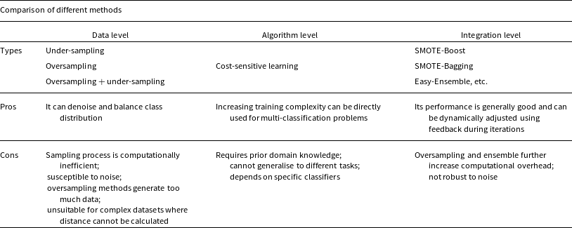

Figure 1. Folded light curves of different kinds of variable stars reported in magnitudes as a function of phase. The data points are represented in light blue dots along with the error bars, and the fitted light curves are illustrated in purple lines.
3. The method
3.1. Imbalanced learning
The existing traditional imbalanced learning algorithms can be categorised into three types: data-level, algorithm-level and integration-level methods. The advantages and disadvantages (Liu et al. Reference Liu2020) of each method are summarised in Table 2. The main reason why the existing methods fail in such tasks is that they ignore the difficulties inherent in the nature of imbalanced learning. These difficulties may arise from the data collection process (such as noise and missing values), or from the characteristics of the dataset (such as class overlap and large data volume), or from the machine learning model (the model capacity is too small or too large) and the task itself (class imbalance). Besides the class imbalance, these factors also significantly degrade the classification performance. Their impact can be further amplified by the high imbalance ratio. Traditional imbalanced learning methods usually only address one or several of these factors, and the final performance depends on the choice of hyperparameters. For instance, the number of neighbours considered in the distance-based re-sampling will affect the sensitivity to noise (Liu et al. Reference Liu2020). The cost matrix in the cost-sensitive learning needs to be set by experts. Since SPE (Liu et al. Reference Liu2020) does not require any predefined distance metric or computation, it is more convenient for application and more efficient for computation. Moreover, SPE is adaptive to different models and robust to noises and missing values.
In this paper, we use SPE to classify the variables. Fig. 2 illustrates the SPE framework. Compared with traditional methods, it has some advantages as follows (Liu et al. Reference Liu2020):
-
1. It can get better classification performance.
-
2. It uses less training data.
-
3. For sampling, it requires less computation time.
-
4. It is robust for data with noise or missing values.
-
5. Compared to traditional imbalanced learning, SPE is less influenced by hyperparameters since it belongs to ensemble learning methods.
-
6. It provides various base classifiers for choice.
-
7. It does not depend on the distance metric and can also be applied for discrete data without modification.

Figure 2. The pipeline of Self-paced Ensemble from Liu et al. (Reference Liu2020). Instead of simply balancing the data or directly adjusting class weights, classification hardness is taken into account over the dataset, and the most informative majority data samples are iteratively selected according to the hardness distribution. The under-sampling strategy is controlled by a self-paced procedure, which enables SPE to gradually focus on the harder data samples but still retains the information of the majority sample to prevent over-fitting.
The SPE algorithm introduces the concept of ‘classification hardness distribution’, which reflects the task difficulty related to factors such as noise, model capacity, and class imbalance. Instinctively, hardness means the difficulty of accurately classifying a sample with a classifier. So hardness distribution is helpful to guide the re-sampling strategy to obtain better performance. Rather than simply balancing dataset or directly assigning class weights, the distribution of classification hardness is taken into account, and SPE iteratively selects the most informative majority datasets based on the hardness distribution. Boosting-like serial training is performed using under-sampling and ensemble strategy, and finally an additive model is obtained. Specifically, the under-sampling is controlled by a self-paced procedure, which makes the structure gradually concentrate on the harder samples (i.e., minority sample). All the majority samples are split into k bins based on their hardness values. To harmonise the hardness contribution of each bin, the sample probability of those bins gradually decreases for the majority samples and the declining level is controlled by a self-paced factor. In the first few iterations, the framework primarily focuses on informative samples. In the later iterations when a self-paced factor becomes very large, the information of the majority sample is still retained to prevent over-fitting. So SPE is an efficient, general-purpose, and robust ensemble imbalanced learning algorithm. Now SPE is a part of imbalanced-ensemble toolbox, built on the basis of both scikit-learn (Pedregosa et al. Reference Pedregosa2011) and imbalanced-learn.Footnote b So SPE is directly utilised from the imbalanced-ensemble package in our work.
3.2. Feature extraction
In time-domain astronomy, the data collected from telescopes are usually expressed in the form of light curves. These light curves show the brightness changes of stars over a period of time. The extraction of light curve features is a part of this work, which can be used to characterise and distinguish different variables. Features can range from basic statistical attributes such as mean and standard deviation, to more complex time series features such as autocorrelation functions. Ideally, these features should be informative and discriminative, enabling machine learning algorithms to distinguish the categories of light curves. FATS (Nun et al. Reference Nun2015) is used for feature extraction. We select the features that can best capture the properties of the light curves for imbalanced classification of periodic variable stars.
We choose seven features for classification. They are mean magnitude, standard deviation, mean variance, skew, kurtosis, amplitude, and period. Six of these features are computed by FATS, and the period is from the downloaded catalogue. These features reflect the location, scale, variability, morphology, and observation time of the light curves. They are easy to interpret and robust against bias.
3.3. Hyperparameter optimisation
In previous works, researchers usually used the greedy grid search for hyperparameter optimisation. Hutter, Hoos, & Leyton-Brown (Reference Hutter, Hoos and Leyton-Brown2011) found that Bayesian optimisation, also called sequential model-based optimisation (SMBO), outperformed grid search for large parameter spaces. Compared to SMBO, grid search has slower speed and more computation cost. Moreover, it is affected by setting range of each hyperparameter. In reality, it is impossible to try all possible values of hyperparameters. Considering these factors, we adopt SMBO for selecting optimal hyperparameters. In this work, SMBO is combined with the SPE algorithm to establish a better classifier at high speed.
Table 3. Confusion matrix of binary classification.

3.4. Evaluation metric
For imbalanced learning, the accuracy is not a good measure of the performance of a classifier. So, we usually use other evaluation metrics based on true positive (TP), false negative (FN), false positive (FP), and true negative (TN). For the binary classification, they can be recorded in a confusion matrix, as shown in Table 3. For evaluating the performance of algorithms, Recall and Precision are commonly used. For imbalanced datasets, we also consider Balanced Accuracy, $G-Mean$
(harmonic or geometric mean of Precision and Recall; García, Sánchez, & Mollineda Reference García, Sánchez and Mollineda2007), and AUCROC (the area under receiver operator characteristic curve; Sahiner et al. Reference Sahiner, Chen, Pezeshk and Petrick2017).
$G-Mean$
(harmonic or geometric mean of Precision and Recall; García, Sánchez, & Mollineda Reference García, Sánchez and Mollineda2007), and AUCROC (the area under receiver operator characteristic curve; Sahiner et al. Reference Sahiner, Chen, Pezeshk and Petrick2017).
 \begin{equation} Recall = \frac{TP}{TP+FN} \end{equation}
 \begin{equation} Precision = \frac{TP}{TP+FP} \end{equation}
 \begin{equation} Specificity = \frac{TN}{FP+TN} \end{equation}
 \begin{equation} Balanced\,Accuracy= \frac{Recall+Specificity}{2} \end{equation}
 \begin{equation} G\,Mean=\sqrt{Recall \times Precision}\end{equation}
4. Results and discussion
Our aim is to classify periodic variables based on the CRTS database. Sample imbalance and the performance of a classifier may influence classification results. Our work involves the imbalance problem. Here, we plan to apply the SPE algorithm and Voting Classifier to solve it.
The samples are randomly split into training and test sets for 10 times, with a ratio of 7:3. For the SPE algorithm, it can be used to boost any canonical classifier’s performance (e.g., SVM, C4.5 Quinlan Reference Quinlan1986, Random Forest, or Neural Networks Haykin Reference Haykin2009). Random Forest is selected as the base classifier in our work. Because the number of base classifiers ( $n\_estimators$
) significantly influences the performance of ensemble methods,
$n\_estimators$
) significantly influences the performance of ensemble methods, $n\_estimators$
should be tuned. We use SMBO to select the optimal number of base classifiers.
$n\_estimators$
should be tuned. We use SMBO to select the optimal number of base classifiers.
4.1. Comparing SPE with hierarchical tree classifier
Reference Hosenie, Lyon, Stappers, Mootoovaloo and McBrideHo20 proposed a hierarchical tree classifier (HTC) with three layers for periodic variables using the CRTS catalog. They argued that simple under-sampling methods were not enough to deal with the class imbalance problem. Instead, they applied GpFit (Williams & Rasmussen Reference Williams and Rasmussen2006) to generate artificial data and increase the number of training samples. They used GpFit for data augmentation and Random Forest as the base algorithm for each layer of the HTC. This approach combined data-level and algorithm-level solutions for imbalanced learning. In contrast, our work uses a self-paced under-sampling procedure that gradually focuses on the harder samples and prevents over-fitting. We train and test the SPE algorithm directly on the original data without building a HTC or augmenting the data. To compare the performance of Reference Hosenie, Lyon, Stappers, Mootoovaloo and McBrideHo20’s method and our SPE method, we use AUCROC as a comprehensive metric that reflects the trade-off between sensitivity and specificity. We find that Reference Hosenie, Lyon, Stappers, Mootoovaloo and McBrideHo20’s method performs poorly for classes with small sample sizes, such as Rotational, RRd, Type-II Cepheid, and Blazhko RR Lyrae variables. Fig. 3 shows that our SPE method significantly improves the performance for Blazhko RR Lyrae variables but slightly worse for RRc variables. We also use confusion matrices to compare the methods, as shown in Figs. 4–5. For Reference Hosenie, Lyon, Stappers, Mootoovaloo and McBrideHo20’s method, the HTC divides all variables into Eclipsing, Rotational, and Pulsating variables in the first layer, with Recall values of 72%, 67%, and 88%, respectively. These values are not very high, and any misclassification in this layer will propagate to the next layers. For the second layer, the classification of Eclipsing and Pulsating variables seems good, but it may be influenced by the previous layer. For the third layer, Fig. 5 shows poor performance for separating RRd and Blazhko variables. In fact, for Reference Hosenie, Lyon, Stappers, Mootoovaloo and McBrideHo20’s method, misclassification accumulates from the top layer to the bottom layer. Therefore, the final classification metrics should be computed by multiplying the metrics obtained in three layers. Compared to Reference Hosenie, Lyon, Stappers, Mootoovaloo and McBrideHo20’s method, our SPE method improves the classification Recall of Blazhko RR Lyrae stars from 12% to 85% and of mixed-mode RR Lyrae variables from 29% to 64%; for detached binaries, the classification Recall increases from 68% to 97%; for LPV, the classification Recall rises from 87% to 99%. The only exceptions are RRab, RRc, and contact and semi-detached binary classes.

Figure 3. The AUCROC of SPE for different classes.

Figure 4. Comparison of confusion matrix of SPE with the first-layer classifier of Reference Hosenie, Lyon, Stappers, Mootoovaloo and McBrideHo20.

Figure 5. Confusion matrix of the second-layer and third-layer classifier in Reference Hosenie, Lyon, Stappers, Mootoovaloo and McBrideHo20.
There are some evaluation metrics for imbalanced problems. Here, we consider $Balanced\,Accuracy$
and
$Balanced\,Accuracy$
and $G\,Mean$
. Tables 4–5 represent
$G\,Mean$
. Tables 4–5 represent $Balanced\,Accuracy$
and
$Balanced\,Accuracy$
and $G\,Mean$
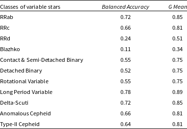
for SPE and the method of Reference Hosenie, Lyon, Stappers, Mootoovaloo and McBrideHo20. We observe that our SPE method increases
$G\,Mean$
for SPE and the method of Reference Hosenie, Lyon, Stappers, Mootoovaloo and McBrideHo20. We observe that our SPE method increases $Balanced\,Accuracy$
of Blazhko stars from 11% to 60% and of RRd stars from 24% to 60%. However, this improvement comes with a slight decrease in the classification of RRab and RRc subtypes. For detached binaries, our SPE method improves
$Balanced\,Accuracy$
of Blazhko stars from 11% to 60% and of RRd stars from 24% to 60%. However, this improvement comes with a slight decrease in the classification of RRab and RRc subtypes. For detached binaries, our SPE method improves $Balanced\,Accuracy$
from 52% to 87% and
$Balanced\,Accuracy$
from 52% to 87% and $G\,Mean$
from 75% to 93%. For rotational variables, our SPE method performs worse than Reference Hosenie, Lyon, Stappers, Mootoovaloo and McBrideHo20’s method, because we separate rotational variables from all the subtypes in one step, while Reference Hosenie, Lyon, Stappers, Mootoovaloo and McBrideHo20’s method uses a three-layer HTC. If we use a similar HTC as Reference Hosenie, Lyon, Stappers, Mootoovaloo and McBrideHo20, Recall of Eclipsing, Rotational, and Pulsating variables by our SPE method is 69%, 73%, and 89%, respectively. Recall (73%) of Rotational variables by our SPE method is higher than that (67%) of Reference Hosenie, Lyon, Stappers, Mootoovaloo and McBrideHo20’s method. Therefore, our approach significantly improves the classification performance compared to Reference Hosenie, Lyon, Stappers, Mootoovaloo and McBrideHo20’s work and achieves good results for most classes of variables except RRab, RRc, and contact and semi-detached binary.
$G\,Mean$
from 75% to 93%. For rotational variables, our SPE method performs worse than Reference Hosenie, Lyon, Stappers, Mootoovaloo and McBrideHo20’s method, because we separate rotational variables from all the subtypes in one step, while Reference Hosenie, Lyon, Stappers, Mootoovaloo and McBrideHo20’s method uses a three-layer HTC. If we use a similar HTC as Reference Hosenie, Lyon, Stappers, Mootoovaloo and McBrideHo20, Recall of Eclipsing, Rotational, and Pulsating variables by our SPE method is 69%, 73%, and 89%, respectively. Recall (73%) of Rotational variables by our SPE method is higher than that (67%) of Reference Hosenie, Lyon, Stappers, Mootoovaloo and McBrideHo20’s method. Therefore, our approach significantly improves the classification performance compared to Reference Hosenie, Lyon, Stappers, Mootoovaloo and McBrideHo20’s work and achieves good results for most classes of variables except RRab, RRc, and contact and semi-detached binary.
Table 4. Mean $Balanced\,Accuracy$
and
$Balanced\,Accuracy$
and $G\,Mean$
for SPE.
$G\,Mean$
for SPE.
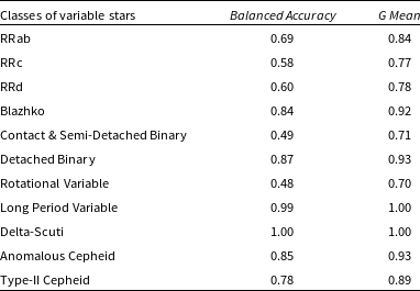
Table 5. Mean $Balanced\,Accuracy$
and
$Balanced\,Accuracy$
and $G\,Mean$
for the work of Reference Hosenie, Lyon, Stappers, Mootoovaloo and McBrideHo20.
$G\,Mean$
for the work of Reference Hosenie, Lyon, Stappers, Mootoovaloo and McBrideHo20.
To summarise, the SPE algorithm can classify all the variables in one step without using HTC, and its ability to increase Recall makes it desirable. The results show that the SPE algorithm favours the small sample classes, such as RRd, Blazhko, Delta-scuti, and Cepheid stars, and achieves high classification performance for them. However, the base algorithm of HTC is Random Forest, which is similar to other traditional classifiers and tends to select the majority classes, such as RRab and RRc stars. Therefore, there is a trade-off between SPE and Random Forest. To balance their performance, we will use a Voting Classifier that combines SPE and Random Forest in Section 4.2.
4.2. Voting Classifier
The Voting Classifier is a method that combines different machine learning classifiers and uses a majority vote or the average predicted probabilities (soft vote) to predict the class labels. We use soft voting and return the class label as argmax of the average of predicted probabilities, as explained in the websiteFootnote c and Fig. 6. The voting mechanism may help us to balance the performance between SPE and Random Forest and thus improve the classification accuracy. We build Random Forest and SPE models separately and then use voting to return the class label based on the average predicted probabilities of both models. Figs. 7 and 8 show that Voting Classifier can correct errors made by any individual classifier, leading to better performance. Specifically, Voting Classifier finds a balance between Random Forest and SPE. Compared to the SPE classifier, Voting Classifier increases the classification Recall of the RRab and RRc stars but decreases it for the RRd and Blazhko stars. Compared to Random Forest, Voting Classifier retains some advantages of the SPE classifier. So it can also be sensitive to small sample classes, such as Delta-scuti and Cepheid stars. We also compute $Balanced\,Accuracy$
for Random Forest, SPE, and Voting Classifier, which are 71%, 78%, and 77%, respectively. Table 6 shows that Voting Classifier can balance the performance of classifiers. Therefore, for different research goals, we may adopt different strategies. For large surveys, a comprehensive classifier is necessary, and Voting Classifier is useful to obtain a balanced classification. If we are interested in the small classes, such as Blazhko and Delta-Scuti stars, we may use the SPE classifier. Similarly, if we tend to select the majority classes, we may use the Random Forest algorithm.
$Balanced\,Accuracy$
for Random Forest, SPE, and Voting Classifier, which are 71%, 78%, and 77%, respectively. Table 6 shows that Voting Classifier can balance the performance of classifiers. Therefore, for different research goals, we may adopt different strategies. For large surveys, a comprehensive classifier is necessary, and Voting Classifier is useful to obtain a balanced classification. If we are interested in the small classes, such as Blazhko and Delta-Scuti stars, we may use the SPE classifier. Similarly, if we tend to select the majority classes, we may use the Random Forest algorithm.
4.3. Some factors affecting the performance of a classifier
Since class imbalance is not the fundamental cause of classification difficulty (Liu et al. Reference Liu2020), there are other factors influencing the performance of a classifier, as follows:
-
1. Some minority class samples appear in the distribution of dense majority class samples.
-
2. Overlapping between classes (García et al. Reference García, Sánchez and Mollineda2007).
-
3. Minority class is split into small disjuncts due to sparsity, which is abbreviated as small disjuncts (Prati, Batista, & Monard Reference Prati, Batista and Monard2004).
In our work, overlapping between classes makes it hard for a classifier to separate the minority from the majority. For example, subtypes of RR Lyrae stars overlap because they have no clear physical differences. RRab stars pulsate in fundamental mode while RRc stars pulsate in the first overtone, so they can be separated well. However, RRd stars pulsate in both modes, so they are tricky to distinguish from RRab and RRc stars. Furthermore, Blazhko effect occurs among RRab, RRc, and RRd stars. Fig. 9 shows that it is not easy to separate RRc stars from RRd stars, and RRab from Blazhko stars. Only for show, the scatter plot of Period versus Smallkurtosis is given here, actually it is difficult to distinguish different RR Lyrae stars by any pairwise combination of features due to their overlapping. Rotating variables show small luminosity changes from patches of light spots on their surfaces, and they may have bright spots at the magnetic poles. Moreover, they often belong to binary systems. All these facts lead to the confusion of rotating stars with other classes.

Figure 6. The flowchart of the Voting Classifier. In Soft voting, classifiers or base models are fed with training data to predict the class output of n possibilities. Each classifier independently assigns the occurrence probability of each class. In the end, the average of the possibilities of each class is calculated, and the final output is labelled as the class with maximum average.

Figure 7. Confusion matrix of SPE.

Figure 8. A Voting Classifier is built by combining Random Forest and SPE. As shown in Fig. 7, the left and right panels depict the confusion matrices of Random Forest and Voting Classifier, respectively.
Table 6. Mean $Balanced\,Accuracy$
and
$Balanced\,Accuracy$
and $G\,Mean$
for Voting Classifier.
$G\,Mean$
for Voting Classifier.


Figure 9. The Period versus Smallkurtosis distribution of RRab, RRc, RRd, and Blazhko stars.
Another reason is that the labels of periodic variables depend on the classification of existing sky surveys or different experts. The classifier’s performance will suffer from the wrong labels. If the standard variable star sets or accurate labels are provided, the classifier will obtain a more reliable performance.
As a result, the SPE algorithm is suitable for the classification task of targeting minority samples, compared to traditional imbalanced learning. By combining SPE with Random Forest in a Voting Classifier, we can achieve better balanced classification performance.
5. Conclusion
In this work, we use the SPE algorithm and Voting Classifier to classify different variables and address the imbalanced classification problem. Compared to Reference Hosenie, Lyon, Stappers, Mootoovaloo and McBrideHo20’s work, which uses GpFit for data augmentation and Random Forest for hierarchical classification, our SPE method uses the original dataset without data processing and classifies all variables in one step. Moreover, our SPE method avoids the propagation of misclassification from one layer to another in the hierarchical trees. Therefore, our SPE method is better when these factors are considered. The results also show that the SPE algorithm improves the performance for minority classes at the expense of some majority classes without losing the overall accuracy. Considering the trade-off between SPE and Random Forest, we use the Voting Classifier to balance the overall classification performance. In practice, the overlapping of classes and inconsistent labels may lead to misclassification and affect the performance of classifiers. Therefore, a complete and representative known sample is essential for building an excellent classifier. However, such samples are scarce, especially for rare objects. In this case, the SPE algorithm shows its superiority. For the identification of minority classes, the SPE algorithm and Voting Classifier are efficient and reliable, and they can be applied to the time-domain data of other larger sky survey projects (LSST, etc.).
Acknowledgements
We are grateful to the anonymous referee for the constructive comments, which significantly helps improve our paper. This paper is funded by the National Natural Science Foundation of China under grants Nos.12203077, No.12273076, No.12133001, and No.11873066, the science research grants from the China Manned Space Project with Nos. CMS-CSST-2021-A04 and CMS-CSST-2021-A06, and Natural Science Foundation of Hebei Province No.A2018106014. We acknowledgement the CRTS databases.
Data availability
Variables of the Catalina Surveys DR2 are available from


 Open access