


Introduction
The information obtained from molecular dynamics (MD) simulations of protein–ligand complexes can be leveraged to predict enzymatic activity. The most common strategy is to use the MD trajectory to compute the binding energy of the complex, which is expected to be correlated with the enzymatic activity (Limongelli, Reference Limongelli2020). The main challenge of calculating binding energies from simulations is that enough conformational space needs to be explored, making the approach expensive (Li and Gilson, Reference Li and Gilson2018). Another strategy is to directly analyse how the ligand interacts with the enzyme during the simulation. The behaviour of the complex of interest during the simulation can hint to how well the enzyme will be able to accommodate the ligand, and hence catalyse the reaction (Bruice, Reference Bruice2002; Voss et al., Reference Voss, Das, Genz, Kumar, Kulkarni, Kustosz, Kumar, Bornscheuer and Höhne2018; Ramírez-Palacios et al., Reference Ramírez-Palacios, Wijma, Thallmair, Marrink and Janssen2021). However, identification of the set of geometric criteria that can distinguish good from bad ligands or enzymes is a laborious task.
Deep learning (DL) can help in the identification of interesting molecular events taking place during an MD simulation (Berishvili et al., Reference Berishvili, Perkin, Voronkov, Radchenko, Syed, Venkata Ramana Reddy, Pillay, Kumar, Choonara, Kamal and Palyulin2019; Terao, Reference Terao2020; Wang et al., Reference Wang, Lamim Ribeiro and Tiwary2020). The main advantage of DL is the reduced manual intervention needed to perform analysis of data, often yielding better accuracies than traditional methods (i.e. hard-coded algorithms). The high-dimensionality of MD trajectories complicates any analysis, and DL can help alleviate this factor by, for example, meaningfully projecting the high-dimensional (high-d) trajectory into a low-d space to facilitate visualisation and analysis (Taufer et al., Reference Taufer, Estrada and Johnston2020; Frassek et al., Reference Frassek, Arjun and Bolhuis2021; Glielmo et al., Reference Glielmo, Husic, Rodriguez, Clementi, Noé and Laio2021). There are several possibilities for projecting simulations into low-d representations, but which one to use will depend on the type of representation used to describe the trajectories. For example, one can view trajectories as a regular-grid of pixels (images), and use the repertory of computer vision machine learning methods to perform the desired task. Or one can view trajectories as time-series data, and use DL to perform time-series forecasting.
The architecture of excellence in DL is the convolutional neural network (CNN; LeCun et al., Reference LeCun, Boser, Denker, Henderson, Howard, Hubbard and Jackel1989). CNNs work by sequentially performing convolution operations on subsets of pixels across the entire input image. The convolution operation between an input signal, $ f $
, and a filter,
$ f $
, and a filter, $ g $
, can be computed as:
$ g $
, can be computed as: $ {s}_t={\left(f\star g\right)}_t={\sum}_{a=-\propto}^{a=\propto}\hskip2pt {f}_{(a)}{g}_{\left(a+t\right)} $
, where
$ {s}_t={\left(f\star g\right)}_t={\sum}_{a=-\propto}^{a=\propto}\hskip2pt {f}_{(a)}{g}_{\left(a+t\right)} $
, where $ {s}_t $
is the feature map. The filter,
$ {s}_t $
is the feature map. The filter, $ g $
, is learned through training. The most popular CNN is 2D-CNN, which works on 2D images, but a simplified version, the 1D-CNN, is more appropriate for trajectories (Jiang and Zavala, Reference Jiang and Zavala2021). A 3D-CNN has also been proposed (Tran et al., Reference Tran, Bourdev, Fergus, Torresani and Paluri2015) to be used in molecular representations but it is not as common (Fukuya and Shibuta, Reference Fukuya and Shibuta2020). In this work, both 1D-CNN and 2D-CNN are used to analyse the MD trajectories.
$ g $
, is learned through training. The most popular CNN is 2D-CNN, which works on 2D images, but a simplified version, the 1D-CNN, is more appropriate for trajectories (Jiang and Zavala, Reference Jiang and Zavala2021). A 3D-CNN has also been proposed (Tran et al., Reference Tran, Bourdev, Fergus, Torresani and Paluri2015) to be used in molecular representations but it is not as common (Fukuya and Shibuta, Reference Fukuya and Shibuta2020). In this work, both 1D-CNN and 2D-CNN are used to analyse the MD trajectories.
Additionally, analysis of MD simulations by DL algorithms can be done through time-series forecasting. Time-series forecasting aims to making predictions about the future values of a series based on its history (e.g. predict tomorrow’s temperature given historical weather data of temperature and humidity). Recurrent neural networks (RNNs) are the standard architecture for time-series forecasting (Petneházi, Reference Petneházi2019; Hewamalage et al., Reference Hewamalage, Bergmeir and Bandara2021). A potential pitfall of RNN-based models is that they can suffer from vanishing or exploding gradients if the distance from the input to the output layers becomes too large (Bengio et al., Reference Bengio, Simard and Frasconi1994). The most popular RNNs are long short-term memory (LSTM; Hochreiter and Schmidhuber, Reference Hochreiter and Schmidhuber1997) and the simpler gated recurrent unit (GRU; Chung et al., Reference Chung, Gulcehre, Cho and Bengio2014). Both LSTM and GRU use gating units to control the flow of information from the distant past to the distant future, preventing degradation of the input signal (Sherstinsky, Reference Sherstinsky2020). A promising alternative for long sequences are attention-based architectures (Vaswani et al., Reference Vaswani, Shazeer, Parmar, Uszkoreit, Jones, Gomez, Kaiser and Polosukhin2017). Autoencoders (AEs) have also been used for time-series forecasting of MD trajectories (e.g. time-lagged AEs), where the aim of the AE is not to reproduce the current but a future simulation frame (Wehmeyer and Noé, Reference Wehmeyer and Noé2018). The LSTM architecture was chosen to model the time-series, because of its ability to identify patterns at multiple frequencies (Lange et al., Reference Lange, Brunton and Kutz2020), and molecular events emerge from the combination of molecular motions taking place at different time scales. A neural network trained on a time-series forecasting task may implicitly learn to separate trajectories in classes. Then, projecting the latent space representations of the trajectories into some orthogonal vector in a way that reproduces proximity or passing the embeddings through a dense layer should allow for binary classification. Algorithms for making meaningful projections from high-d to low-d representations are principal component analysis (PCA; Wold et al., Reference Wold, Esbensen and Geladi1987), time-independent component analysis (TICA; Molgedey and Schuster, Reference Molgedey and Schuster1994), t-distributed stochastic neighbour embedding (t-SNE; van der Maaten and Hinton, Reference van der Maaten and Hinton2008), among others (Das et al., Reference Das, Moll, Stamati, Kavraki and Clementi2006; Ceriotti et al., Reference Ceriotti, Tribello and Parrinello2011; Ferguson et al., Reference Ferguson, Panagiotopoulos, Kevrekidis and Debenedetti2011; Spiwok and Králová, Reference Spiwok and Králová2011; Tribello et al., Reference Tribello, Ceriotti and Parrinello2012; Noé and Clementi, Reference Noé and Clementi2015; Chen and Ferguson, Reference Chen and Ferguson2018; Lemke and Peter, Reference Lemke and Peter2019; Spiwok and Kříž, Reference Spiwok and Kříž2020). t-SNE aims to reproduce proximities rather than distances (PCA) or divergences (TICA).
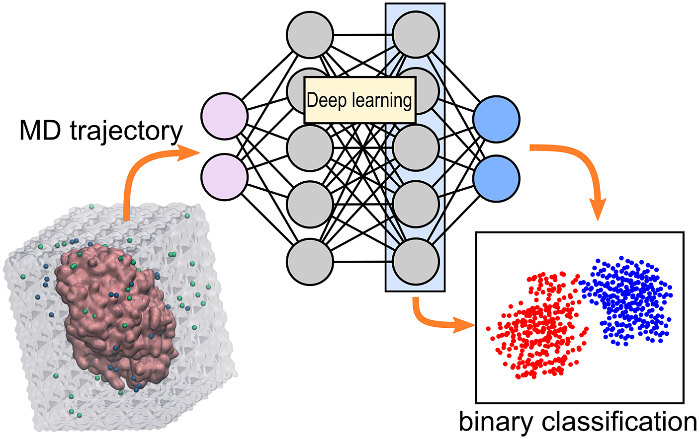
ω-Transaminases are pyridoxal-5′-phosphate (PLP)-dependent enzymes that can catalyse the conversion of chiral amines from more accessible achiral ketones (Cassimjee et al., Reference Cassimjee, Manta and Himo2015). ω-Transaminases are desirable catalysts in industry for the production of chiral amines but the substrate scope and selectivity usually need to be fine-tuned to the molecule of interest (Breuer et al., Reference Breuer, Ditrich, Habicher, Hauer, Keßeler, Stürmer and Zelinski2004; Kelly et al., Reference Kelly, Pohle, Wharry, Mix, Allen, Moody and Gilmore2018). Hence, the development of computational algorithms to predict the selectivity of ω-transaminases can accelerate enzyme design and discovery campaigns. Previously, we presented a framework for predicting the enantiopreference of an ω-transaminase from Vibrio fluvialis (Vf-TA; Ramírez-Palacios et al., Reference Ramírez-Palacios, Wijma, Thallmair, Marrink and Janssen2021). The approach consisted in counting the number of near-attack conformations (NACs) observed during MD trajectories to quantitatively predict the enantiopreference of the enzyme towards a given ligand ( Fig. 1a). However, some fine-tuning was needed to find appropriate geometric criteria to define a NAC. Herein, we use a machine learning approach to tackle the same problem ( Fig. 1b). The MD trajectories are viewed as vectors consisting of descriptors (distances, angles and dihedrals) and labelled as ‘reactive’ when containing the preferred enantiomer and as ‘non-reactive’ otherwise. The dataset to train the DL models consists of 100 examples per class and per ligand, summing up to a total of (100 × 2 × 49) 9,800 examples, split into training (80%) and validation (20%) datasets. Binary classification is achieved by supervised (CNN) or semi-supervised (LSTM) training of a neural network.
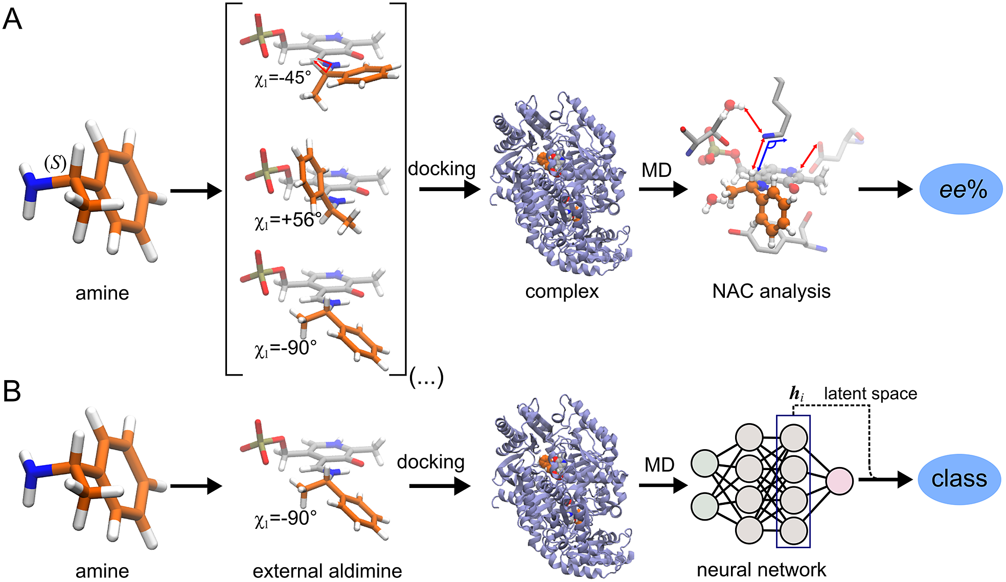
Fig. 1. Computational prediction of the ω-TA selectivity by (a) geometric analysis of near-attack conformations (NACs) and (b) deep learning. In both methodologies, short MD simulations (20 ps) are run using the docked complex as starting conformation. In the NAC-based methodology, presented in Ramírez-Palacios et al. (Reference Ramírez-Palacios, Wijma, Thallmair, Marrink and Janssen2021), a combination of docking and MD simulations was needed to sample through a slow-moving dihedral (χ1). The DL-based methodology, presented in this work, does not necessitate such a strategy of sampling through slow-moving parameters, which reduces the number of MD simulations required. Furthermore, no hand-crafted geometric features are needed for the NN to learn to distinguish between trajectories that contain ‘reactive’ or ‘non-reactive’ enantiomers, which would reduce the number of man-hours required for its implementation to new systems.
The trained CNNs achieved excellent accuracy in the binary classification task. Nonetheless, from a molecular modelling perspective, it is more useful if explanations can also be retrieved from the trained models to identify descriptors that the CNN found to be relevant in achieving the assigned task. Knowledge on the importance of each descriptor can be useful, for example, to refine the set of geometric criteria used to define binding poses or to identify interesting events taking place in the trajectories that might characterise the classes. Many deep-learning models are explainable by design (intrinsic interpretability), while others are built as black boxes and obtaining explanations requires actions (post hoc interpretability; Bodria et al., Reference Bodria, Giannotti, Guidotti, Naretto, Pedreschi and Rinzivillo2021). Owing to the visual nature of the representations used as input to train CNN models (and the maturity of the architecture), convolutional networks allow a more visual description of the decision-making process in the form of saliency maps. A saliency map shows the relative contribution from each input region (pixel) to the final prediction. One of the first saliency maps proposed was class activation map (CAM; Zhou et al., Reference Zhou, Khosla, Lapedriza, Oliva and Torralba2016) but it requires the feature maps to directly precede the softmax layers (which means that not every topology allows this type of saliency map). CAM was later improved to gradient-weighted class activation map (Grad-CAM) and guided Grad-CAM (Selvaraju et al., Reference Selvaraju, Cogswell, Das, Vedantam, Parikh and Batra2017). Other saliency maps worth mentioning are LIME (Ribeiro et al., Reference Ribeiro, Singh and Guestrin2016), RISE (Petsiuk et al., Reference Petsiuk, Das and Saenko2018), IntGrad (Sundararajan et al., Reference Sundararajan, Taly and Yan2017) and SmoothGrad (Smilkov et al., Reference Smilkov, Thorat, Kim, Viégas and Wattenberg2017). Bodria et al. (Reference Bodria, Giannotti, Guidotti, Naretto, Pedreschi and Rinzivillo2021) provide an excellent up-to-date review on explanation methods.
Methods
MD simulations
Enzyme–ligand complexes obtained by Rosetta docking were used as starting conformations for 20 ps-long atomistic MD simulations. The enzyme is the wild-type Vf-TA (PDB: 4E3Q), and the ligand is the external aldimine intermediate of a set of 49 compounds (Fig. 2, Fig. 3). Exact details about the methodology for running the MD simulations was presented in Ramírez-Palacios et al. (Reference Ramírez-Palacios, Wijma, Thallmair, Marrink and Janssen2021).

Fig. 2. Structures of the compounds used in this study. The ligands were the external aldimine form of the amines shown in the figure. Following CIP rules, all compounds shown are (S)-enantiomers, except 32, 33, 35, 36 and 45 which formally are (R)-enantiomers.
Dataset construction
The dataset was constructed from 9,800 MD trajectories (100 per ligand), half belonging to the class labelled as ‘reactive’ and the other half to the class ‘non-reactive’. The trajectories containing the preferred enantiomer [typically the (S)-enantiomer] were labelled as ‘reactive’, whereas the trajectories containing the non-preferred enantiomer [typically the (R)-enantiomer] were labelled as ‘non-reactive’. The input tensors used for training the DL models consisted of 15 descriptors (distances, angles and dihedrals) taken from each 1,000-frame trajectory (20 ps of simulation), $ {\boldsymbol{x}}_i\in {\mathbb{R}}^{N\times F} $
, where
$ {\boldsymbol{x}}_i\in {\mathbb{R}}^{N\times F} $
, where $ N $
is the number of timesteps and
$ N $
is the number of timesteps and $ F $
is the number of descriptors per trajectory. The descriptors are distances, angles or dihedrals that are considered important for the transamination reaction to take place (Fig. 3, Fig. 4; Cassimjee et al., Reference Cassimjee, Manta and Himo2015). Descriptors relating to a water molecule near Lys285 and Thr322 were also included. Some descriptors are redundant (e.g. d
5 and d
6). The training dataset was split into training (80%) and validation sets (20%). To facilitate – but not guarantee – generalisation to unseen ligands, the split between training and validation sets was not random but ligand-dependent: all trajectories containing ligands 01–38 were assigned to the training dataset, and all trajectories containing ligands 39–49 were assigned to the validation dataset.
$ F $
is the number of descriptors per trajectory. The descriptors are distances, angles or dihedrals that are considered important for the transamination reaction to take place (Fig. 3, Fig. 4; Cassimjee et al., Reference Cassimjee, Manta and Himo2015). Descriptors relating to a water molecule near Lys285 and Thr322 were also included. Some descriptors are redundant (e.g. d
5 and d
6). The training dataset was split into training (80%) and validation sets (20%). To facilitate – but not guarantee – generalisation to unseen ligands, the split between training and validation sets was not random but ligand-dependent: all trajectories containing ligands 01–38 were assigned to the training dataset, and all trajectories containing ligands 39–49 were assigned to the validation dataset.
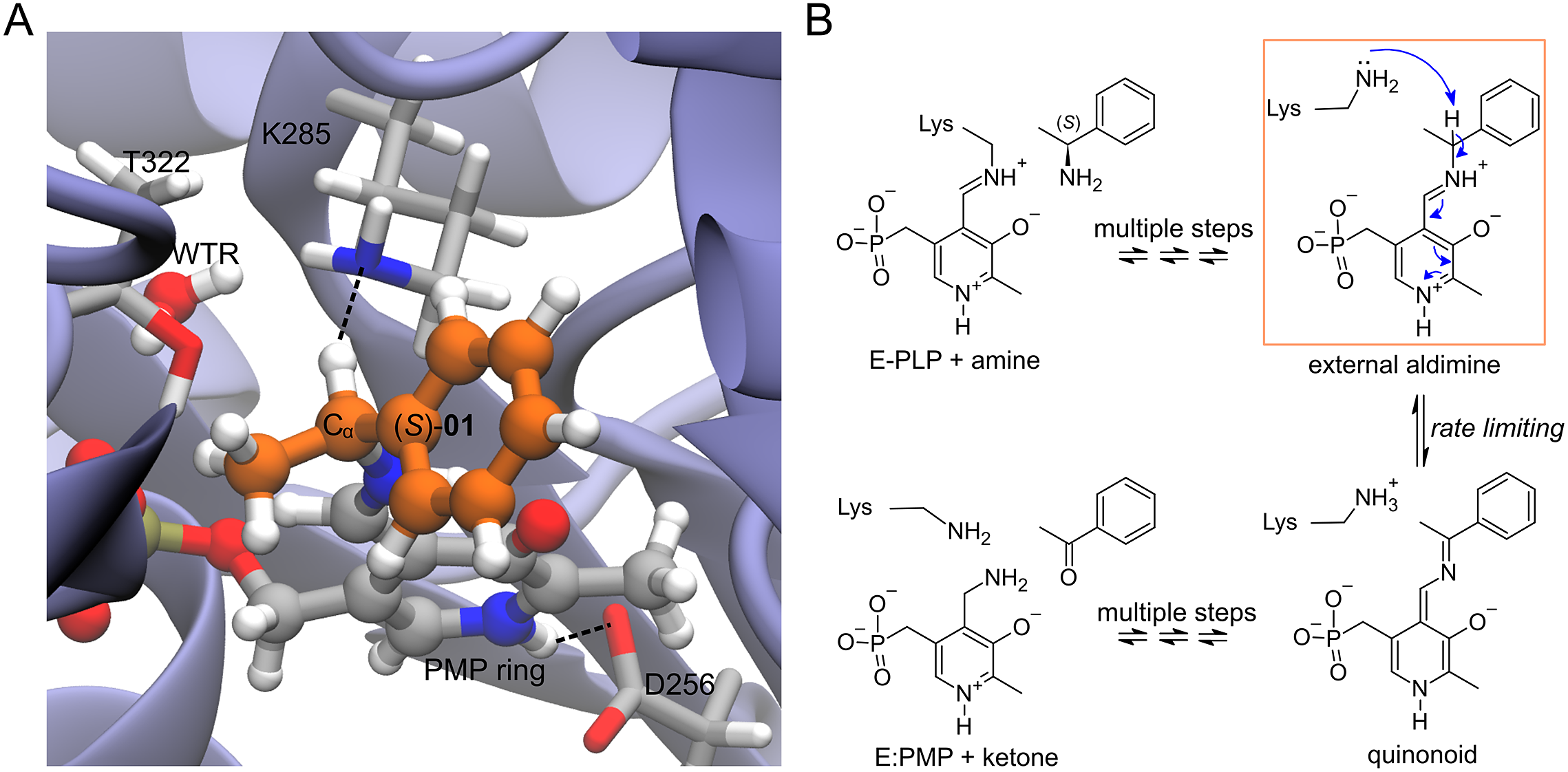
Fig. 3. (a) Structure of the complex of Vf-TA with the external aldimine intermediate of compound (S)-01. (b) Transamination reaction. The fully reversible transamination reaction consists of multiple steps in which an amino group is transferred from the substrate to the cofactor or, in the reverse direction, from the cofactor to the substrate. Among the reaction intermediates, we only modelled the external aldimine intermediate, because it is most likely involved in the rate-limiting step of the reaction. In this step, the nucleophilic proton abstraction of the external aldimine by the catalytic lysine leads to the formation of the quinonoid intermediate. Short MD simulations of the external aldimine intermediate complex were used as input for the neural networks, which were tasked with classifying them.
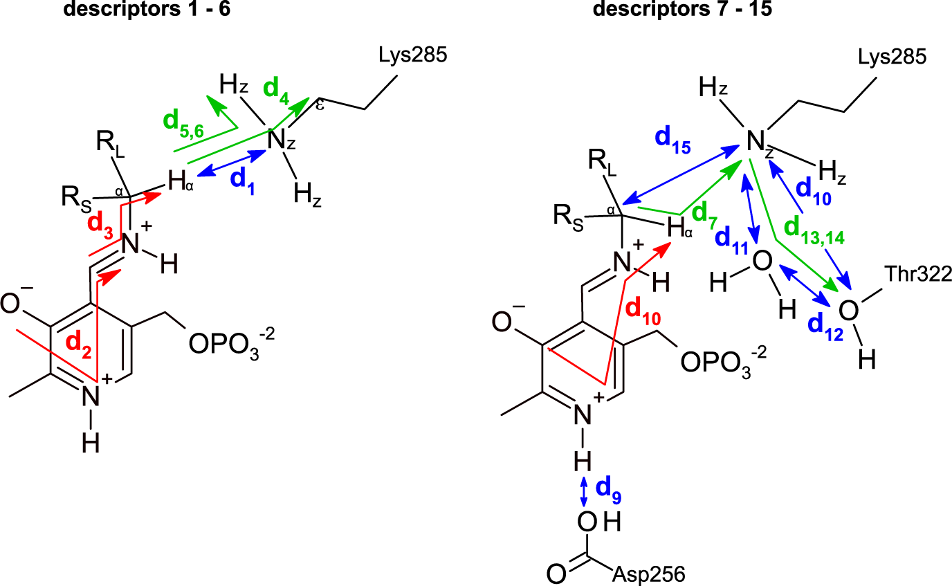
Fig. 4. Descriptors used to represent the MD trajectories. Colour codes are: blue, distances; green, angles; red, dihedrals. The 15 descriptors are shown in two parts only for clarity.
Class labels
Each trajectory was labelled as either ‘reactive’ or ‘non-reactive’, depending exclusively on whether the ligand contained in the complex was the preferred enantiomer (class ‘reactive’) or the non-preferred enantiomer (class ‘non-reactive’). The label is referring to whether the ligand can be accommodated by Vf-TA and lead to catalysis. Typically for Vf-TA, the (S)-enantiomer is the preferred enantiomer (Fig. 2). The assumption is that all simulations obtained from the preferred enantiomer would behave similar among each other but dissimilar from the simulations of the opposite enantiomer, and vice versa. Here, the word similar is in terms of the metric found by the neural network to better accomplish the binary classification task.
Network building and training procedure
All models were built using the TensorFlow 2.4 library (Abadi et al., Reference Abadi, Barham, Chen, Chen, Davis, Dean, Devin, Ghemawat, Irving, Isard, Kudlur, Levenberg, Monga, Moore, Murray, Steiner, Tucker, Vasudevan, Warden, Wicke, Yu and Zheng2016; sequential API). Unless otherwise indicated, all layers use the rectified linear unit (ReLU) activation function. Hereby a description of the construction and training procedure for the CNN (1D- and 2D-CNN) and LSTM models for the binary classification of MD trajectories, as well as the CAM and latent space visualisation (Fig. 5).

Fig. 5. Configuration of the NNs used to classify the MD trajectories. Each trajectory consists of 1,000 frames and each frame is represented by 15 descriptors (distances, angles and dihedrals thought to be relevant in the studied reaction). (a) In the 1D-CNN model, an MD trajectory is treated as a signal with multiple channels (descriptors). The input signal (sized 1,000 × 15) passes through multiple convolutional, pooling and dense layers until the final neuron outputs 0 or 1 to represent the class ‘non-reactive’ or ‘reactive’, respectively. (b) In the 2D-CNN model, the trajectory is represented as an image of size 1,000 × 15 (binary classification) or 320 × 320 (CAM visualisation), with one colour channel (analogous to a black-and-white picture). The input image passes through multiple convolutional, pooling, dropout and dense layers until the final neuron outputs the class prediction. (c) The LSTM model is trained to predict the next frame based on information from all other frames that came before it. After training, the embeddings obtained from the second LSTM layer are used to predict the trajectory’s class.
1D-CNN model
Input vectors for the 1D-CNN model were of shape [batch,1000,15]. The 1D-CNN model was constructed using the following stack of Keras layers: (1) Conv1D (16 filters, kernel of length 7), (2) MaxPooling1D (size of pooling window = 5), (3) Conv1D (16 filters, kernel of length 7), (4) GlobalMaxPooling1D and (5) Dense (one output unit, sigmoid activation). The network was trained via backpropagation for 10 epochs using the RMSprop (learning rate = 1 × 10⁻⁴) optimiser in minibatches of eight examples. Binary cross-entropy was used as the loss function.
2D-CNN model
Input vectors for the 2D-CNN model were of shape [batch,15,1000,1]. The model was constructed using the following stack of Keras layers: (1) Conv2D (eight filters, kernel of size 1 × 5), (2) MaxPooling2D (pool size = 1 × 3), (3) Dropout (dropout rate = 0.3), (4) Conv2D (four filters, kernel of size 1 × 5), (5) MaxPooling2D (pool size = 1 × 3), (6) Flatten, (7) Dense (one output unit, sigmoid activation). The network was trained in minibatches (size 16) via backpropagation for 20 epochs using the RMSprop (learning rate = 1 × 10⁻⁴) optimiser. Binary cross-entropy was used as the loss function.
LSTM model
The LSTM model was constructed using the following stack of Keras layers: (1) LSTM (16 units, tanh activation function), (2) LSTM (8 units, tanh activation function), (3) Dense (1 output unit, without activation). Input vectors were of shape [batch,50,15]. The network was trained for five epochs using the ADAM optimiser (Kingma and Ba, Reference Kingma and Ba2017; learning rate = 0.01) with a batch size of 128. The dataset contained ~500,000 input vectors. The task of the LSTM model can be simplified as: given the following input vector containing 15 descriptors measured at 50 timesteps ( $ {\boldsymbol{x}}_i\in {\mathbb{R}}^{50\times 15} $
), predict the value of the query descriptor (d
4) at the next timestep (
$ {\boldsymbol{x}}_i\in {\mathbb{R}}^{50\times 15} $
), predict the value of the query descriptor (d
4) at the next timestep ( $ {\hat{\boldsymbol{y}}}_i\in \mathbb{R} $
). The mean-squared error (MSE) between the predicted (
$ {\hat{\boldsymbol{y}}}_i\in \mathbb{R} $
). The mean-squared error (MSE) between the predicted ( $ {\hat{\boldsymbol{y}}}_i $
) and true (
$ {\hat{\boldsymbol{y}}}_i $
) and true ( $ {\boldsymbol{y}}_i $
) label was used as the loss function. After training the LSTM model, the embeddings obtained from the penultimate layer (
$ {\boldsymbol{y}}_i $
) label was used as the loss function. After training the LSTM model, the embeddings obtained from the penultimate layer ( $ {\boldsymbol{h}}_i^{LSTM}\in {\mathbb{R}}^8 $
) were used as input data.
$ {\boldsymbol{h}}_i^{LSTM}\in {\mathbb{R}}^8 $
) were used as input data.
2D-CNN model for CAM visualisation
The 2D-CNN model used to create the activation maps used pixel images as input vectors. The input vectors were created using the ImageDataGenerator Keras class to resize the trajectories to [batch,320,320,1]. The overparameterised model was constructed using the following stack of Keras layers: (1) Conv2D (128 filters, kernel of size 3 × 3), (2) MaxPooling2D (pool size = 2 × 2), (3) Conv2D (64 filters, kernel of size 3 × 3), (4) MaxPooling2D (pool size = 2 × 2), (5) Conv2D (32 filters, kernel of size 3 × 3), (6) MaxPooling2D (pool size = 2 × 2), (7) Conv2D (16 filters, kernel of size 3 × 3), (8) MaxPooling2D (pool size = 2 × 2), (9) Flatten, (10) Dense (256 units) and (11) Dense (one output unit, sigmoid activation). The network was trained in minibatches (size 1) via backpropagation for 20 epochs using the RMSprop (learning rate = 1 × 10⁻⁴) optimiser. Binary cross-entropy was used as the loss function.
Latent space visualisation
A two-dimensional projection of the vector embeddings produced by the penultimate layer of the 1D-CNN ( $ {\boldsymbol{h}}_i\in {\mathbb{R}}^{16} $
) model were produced by t-SNE (t-distributed stochastic network embeddings; van der Maaten and Hinton, Reference van der Maaten and Hinton2008), as implemented in the SkLearn library (Pedregosa et al., Reference Pedregosa, Varoquaux, Gramfort, Michel, Thirion, Grisel, Blondel, Prettenhofer, Weiss, Dubourg, Vanderplas, Passos, Cournapeau, Brucher, Perrot and Duchesnay2011; with perplexity = 30).
$ {\boldsymbol{h}}_i\in {\mathbb{R}}^{16} $
) model were produced by t-SNE (t-distributed stochastic network embeddings; van der Maaten and Hinton, Reference van der Maaten and Hinton2008), as implemented in the SkLearn library (Pedregosa et al., Reference Pedregosa, Varoquaux, Gramfort, Michel, Thirion, Grisel, Blondel, Prettenhofer, Weiss, Dubourg, Vanderplas, Passos, Cournapeau, Brucher, Perrot and Duchesnay2011; with perplexity = 30).
Results and discussion
Dynamics of the studied system
The length of the MD trajectories was capped at only 20 ps to keep the computational cost low, which is useful for its applicability in high-throughput screening. Longer simulations in the order of hundreds of ns can easily differentiate between ‘reactive’ and ‘non-reactive’ enantiomers, because the ‘non-reactive’ enantiomer has enough time to evolve and adopt a non-catalytic orientation (χ1 = d 3 = +90°), whereas the ‘reactive’ enantiomer remains in a catalytic orientation (χ1 = d 3 = −90°; Ramírez-Palacios et al., Reference Ramírez-Palacios, Wijma, Thallmair, Marrink and Janssen2021). However, the initial conformation is mostly retained during the shorter simulations, as shown in Supplementary Fig. 1. We were unable to tell the two classes apart by visual inspection of the trajectories, and wondered whether a NN could.
Distribution of input descriptors
To assess whether a NN is even needed to classify the trajectories, one can first look at the distribution of the input descriptors to see if differences between classes are already present. The distribution of descriptors used as input data shows no difference in distribution between the two classes (Supplementary Fig. 2). This means that any algorithm used for classification of the trajectories cannot rely solely on the position-dependent values of one descriptor, and instead needs a combination of descriptors [as was shown in the previous work (Ramírez-Palacios et al., Reference Ramírez-Palacios, Wijma, Thallmair, Marrink and Janssen2021)] or patterns (e.g. time-dependent changes in position). CNNs can do both, and are thus a good choice to classify the trajectories.
Trained CNNs achieve high accuracy in the binary classification of MD trajectories
The trained CNNs achieved a good accuracy in the binary classification task in both the training and validation datasets (Table 1; see below for the LSTM model). The training and validation datasets contained trajectories from ligands 01–38 and 39–49, respectively. The split between training and validation datasets was done based on the ligand identity instead of randomly, to allow testing the model’s generalisation to unseen ligands. While it is impossible to know for certain whether the probability distribution of the training dataset is large enough to cover every possible ligand, the high accuracy the model achieves in the validation dataset, which contains unseen ligands, does suggest some generalisation. Fig. 6 shows that most ligands in both the training and validation datasets had a low number of misclassified trajectories. For example, ligand 01 had only one misclassified trajectory: the trajectory belonged to the class ‘reactive’ (blue) but the NN incorrectly classified it as belonging to the class ‘non-reactive’ (red). The ligand with the highest number of misclassified trajectories was ligand 35 (see Ramírez-Palacios et al., Reference Ramírez-Palacios, Wijma, Thallmair, Marrink and Janssen2021 for more details on ligands 35 and 36). Most ligands had only a small number of misclassified trajectories, and 11 of them did not have any misclassified trajectory.
Table 1. Results of the tested NNs in the binary classification of MD trajectories

Abbreviations: LSTM, long short-term memory; ROC-AUC, area under the curve of the receiver-operator characteristic curve.

Fig. 6. Bar plot showing the number of misclassified trajectories per ligand molecule when evaluated with the trained 1D-CNN model. We want the number of misclassified trajectories to be small. The total number of trajectories per ligand is 200, half of which are labelled as ‘non-reactive’ and the other half are labelled as ‘reactive’. For example, ligand 06 has 100 trajectories containing the non-preferred enantiomer (class ‘non-reactive’) of which 37 were misclassified (red bars), and 100 trajectories containing the enantiomer preferred by Vf-TA (class ‘reactive’) of which 23 were misclassified (blue bars) by the NN. There are 49 ligands in total, adding up to a total of 9,800 trajectories.
Disentanglement of input channels
After seeing the 1D-CNN model was accurate in the classification of trajectories, an obvious step forward is to understand what the NN is looking at to arrive to a final decision about the class to which the input vector belongs. The simplest would be to determine on which descriptors (input channels) the NN relies the most. However, disentanglement of the input channels is not an easy task (Cui et al., Reference Cui, Wang and Wang2020), because individual channels are not processed individually in a 1D-CNN architecture. For this reason, an ablation study was performed to evaluate the contribution of each channel to the model’s performance. An ablation study consists of evaluating the performance of the model after removing one or more of its components (Sheikholeslami et al., Reference Sheikholeslami, Meister, Wang, Payberah, Vlassov and Dowling2021). To get an overall picture about the importance of each channel, 15 independent 1D-CNNs were constructed, and each were trained and evaluated using only one descriptor as input vector ( $ {\boldsymbol{x}}_i\in {\mathbb{R}}^{N\times 1} $
). While the approach of using one descriptor at a time does not tell the whole story (because it ignores synergies between descriptors), it does give an impression of which descriptors might be important, for example, for the enzymatic reaction to take place. The results of these 15 1D-CNNs are presented in Fig. 7. For the neural network, descriptor d
1 is not a good descriptor by itself to discriminate between the two classes, which is surprising, because d
1 corresponds to the distance from the proton to be abstracted to the attacking atom (H
α – N
z), and thus a close distance would be needed for the reaction to take place. And similarly, neither is the distance between N
z – C
α (d
15) a good descriptor for the classification task. It is important to clarify that this result is only telling us that neither d
1 nor d
15 alone are enough for the NN to do the classification task, but a combination with other descriptors might produce a different outcome. Fig. 7 shows that while the distance from the water molecule to the oxygen in Thr-OH (d
12) is not important, the distance from the same water to the Lys-NH2 is important (d
11). Lys285 is believed to require water assistance for proton abstraction from the external aldimine intermediate, but there is an alternative mechanism that does not require water (Cassimjee et al., Reference Cassimjee, Manta and Himo2015). The descriptor that better achieves a good accuracy is the angle between H
α – N
z – C
E (d
4), which is expected, because Lys285-NH2 needs to be positioned at the correct angle for the nucleophilic proton abstraction to take place. An interesting observation is that the two ‘siblings’ of d
4 [d
5 and d
6, both refer to the same angle (H
α – N
z – H
z; see Fig. 4)] do not achieve the same accuracy as d
4. The observation is interesting, because in the previous protocol (Ramírez-Palacios et al., Reference Ramírez-Palacios, Wijma, Thallmair, Marrink and Janssen2021), the angles between H
α – N
z – H
z1,2 (d
5,6, previously known as θ1 and θ2) were part of the geometric criteria used to define the reactive conformations of interest, but these results suggest that using the angle H
α – N
z – C
E instead might have been a better choice.
$ {\boldsymbol{x}}_i\in {\mathbb{R}}^{N\times 1} $
). While the approach of using one descriptor at a time does not tell the whole story (because it ignores synergies between descriptors), it does give an impression of which descriptors might be important, for example, for the enzymatic reaction to take place. The results of these 15 1D-CNNs are presented in Fig. 7. For the neural network, descriptor d
1 is not a good descriptor by itself to discriminate between the two classes, which is surprising, because d
1 corresponds to the distance from the proton to be abstracted to the attacking atom (H
α – N
z), and thus a close distance would be needed for the reaction to take place. And similarly, neither is the distance between N
z – C
α (d
15) a good descriptor for the classification task. It is important to clarify that this result is only telling us that neither d
1 nor d
15 alone are enough for the NN to do the classification task, but a combination with other descriptors might produce a different outcome. Fig. 7 shows that while the distance from the water molecule to the oxygen in Thr-OH (d
12) is not important, the distance from the same water to the Lys-NH2 is important (d
11). Lys285 is believed to require water assistance for proton abstraction from the external aldimine intermediate, but there is an alternative mechanism that does not require water (Cassimjee et al., Reference Cassimjee, Manta and Himo2015). The descriptor that better achieves a good accuracy is the angle between H
α – N
z – C
E (d
4), which is expected, because Lys285-NH2 needs to be positioned at the correct angle for the nucleophilic proton abstraction to take place. An interesting observation is that the two ‘siblings’ of d
4 [d
5 and d
6, both refer to the same angle (H
α – N
z – H
z; see Fig. 4)] do not achieve the same accuracy as d
4. The observation is interesting, because in the previous protocol (Ramírez-Palacios et al., Reference Ramírez-Palacios, Wijma, Thallmair, Marrink and Janssen2021), the angles between H
α – N
z – H
z1,2 (d
5,6, previously known as θ1 and θ2) were part of the geometric criteria used to define the reactive conformations of interest, but these results suggest that using the angle H
α – N
z – C
E instead might have been a better choice.

Fig. 7. Accuracy obtained by using one input channel for training, $ {\boldsymbol{x}}_i\in {\mathbb{R}}^{N\times 1} $
, and the accuracy obtained by using all the input channels,
$ {\boldsymbol{x}}_i\in {\mathbb{R}}^{N\times 1} $
, and the accuracy obtained by using all the input channels, $ {\boldsymbol{x}}_i\in {\mathbb{R}}^{N\times 15} $
(first bar, labelled as ‘All’). The error bars are standard deviations over five replicas.
$ {\boldsymbol{x}}_i\in {\mathbb{R}}^{N\times 15} $
(first bar, labelled as ‘All’). The error bars are standard deviations over five replicas.
Visualisation of the latent space representations
Visualising the latent space representations ( $ {\boldsymbol{h}}_i $
) onto which the trained models project the input vectors (
$ {\boldsymbol{h}}_i $
) onto which the trained models project the input vectors ( $ {\boldsymbol{x}}_i\boldsymbol{\mapsto}{\boldsymbol{h}}_i,{\boldsymbol{x}}_i\in {\mathbb{R}}^{1000\times 15},{\boldsymbol{h}}_i\in {\mathbb{R}}^{16} $
) is useful, because it can provide visual clues about whether subclasses are present (Fig. 8). The presence of subclasses would indicate that on top of trajectories being different, because they belong to distinct classes, they are also different in some other way. Here, the word different is according to the metric the NN learned through training as best-suited to do the classification task. The latent space visualisation did not reveal any major subclasses for the class ‘reactive’, but was indicative of 3–4 subclasses (i.e. clusters of points separated from each other) for the class ‘non-reactive’ (Fig. 8). However, because the LSTM approach was unsuccessful in the binary classification task (see later), these subclasses were not investigated any further.
$ {\boldsymbol{x}}_i\boldsymbol{\mapsto}{\boldsymbol{h}}_i,{\boldsymbol{x}}_i\in {\mathbb{R}}^{1000\times 15},{\boldsymbol{h}}_i\in {\mathbb{R}}^{16} $
) is useful, because it can provide visual clues about whether subclasses are present (Fig. 8). The presence of subclasses would indicate that on top of trajectories being different, because they belong to distinct classes, they are also different in some other way. Here, the word different is according to the metric the NN learned through training as best-suited to do the classification task. The latent space visualisation did not reveal any major subclasses for the class ‘reactive’, but was indicative of 3–4 subclasses (i.e. clusters of points separated from each other) for the class ‘non-reactive’ (Fig. 8). However, because the LSTM approach was unsuccessful in the binary classification task (see later), these subclasses were not investigated any further.

Fig. 8. t-SNE of the latent space representations ( $ {\boldsymbol{h}}_i\in {\mathbb{R}}^{16} $
) obtained from the penultimate layer of the 1D-CNN model. The evaluations were made in the validation dataset (n = 2,200 examples). The reader can think of the latent space as follows: imagine you show an image of a molecule to a chemist and scan their neurons to see which neurons are active and which are not. You then repeat the experiment with a non-expert in chemistry and compare the two scans. The scans will be different, because the expert can give meaning to the image shown. We expect the scan of the neuron activations of the expert to tell us something about the molecule that is not necessarily encoded in the input image (e.g. whether the molecule is realistic or not), coming from the experience (training) of the expert (neural network). That is latent space.
$ {\boldsymbol{h}}_i\in {\mathbb{R}}^{16} $
) obtained from the penultimate layer of the 1D-CNN model. The evaluations were made in the validation dataset (n = 2,200 examples). The reader can think of the latent space as follows: imagine you show an image of a molecule to a chemist and scan their neurons to see which neurons are active and which are not. You then repeat the experiment with a non-expert in chemistry and compare the two scans. The scans will be different, because the expert can give meaning to the image shown. We expect the scan of the neuron activations of the expert to tell us something about the molecule that is not necessarily encoded in the input image (e.g. whether the molecule is realistic or not), coming from the experience (training) of the expert (neural network). That is latent space.
CAM visualisation
Visualising how a model arrives to a particular decision about the input data can by itself be very useful, sometimes more than the task the model was assigned to perform (see below). Fig. 9 shows the CAM visualisation from the 1D-CNN model. The activations are evenly spread out throughout the trajectory which indicates that the neural network is looking at processes happening throughout the trajectory and not at just some specific portion of it. It also suggests that shorter trajectories (<<20 ps) would be enough to do the classification (Supplementary Fig. 3). An overlap of the input descriptors and the activations produced ( Fig. 9b) shows the dependency of the activations on the input signal. Some activations occur when the descriptor reaches a peak, a dip or a plateau, but the activation comes from all the descriptors taken together as a whole. This type of visualisation can be useful in identifying the temporal location of interesting molecular events.

Fig. 9. (a) Heatmap showing the CAM activations of the 1D-CNN model of one input trajectory, presented as example. The y-axis is the filter number, and the x-axis is the time dimension. (b) CAM activations (heatmap) of filter number 4 overlapped to the input vectors of descriptors 3, 4 and 10 (line plot), along a small 2.0 ps window (x-axis). The y-axis contains the normalised values from each descriptor. The hand-drawn arrows show the direction each descriptor follows. At 1.67 ps, the activations are at their highest, and at 1.55 ps, activations are low. The red rectangle shows a region with little activations but where descriptor 3 looks visually similar to the region in which the activations were at their maximum (~1.67 ps).
Visualisation of 2D-CNN is more illustrative than that of 1D-CNN. For this reason, a second CNN model was trained, this time using a 2D-CNN architecture. The CAM visualisation is presented in Fig. 10. As it can be seen, the neural network activates (yellow) in the regions of the 2D image where a trajectory signal is present. As expected, activations were low in the regions in-between channels.

Fig. 10. (a) Example of an input image of size 320 × 320 pixels, and (b) the CAM produced by the image after passing it through a 2D-CNN. Viridis colourmap: the regions with the lowest activations (low importance) are coloured blue, the regions that produce the highest activations are in yellow and the regions with middle importance are in green. The highest activations come from the pixels containing trajectory information.
As mentioned earlier, disentanglement of the contributions of each input descriptor to the classification is not an easy task. A way to make use of the trained model is to visualise the position-dependent activations of each descriptor. This would be useful, for example, in helping define reactive poses or simply to know which values are preferred. For example, in Supplementary Fig. 2 it is shown that descriptor d 1 has the same distribution in the two classes, which means that one cannot simply choose a cut-off value for d 1 and hard-code a solution for the classification task. Fig. 11 shows that the 1D-CNN model has no apparent position-dependent preference for descriptors d 1, d 8, d 9, d 12 and d 15, as both classes show the same distribution. On the other hand, descriptor d 4, the angle between H α – N z – C E, is preferred to be large for the NN to classify the simulation as ‘reactive’ and small to classify it as ‘non-reactive’. This makes sense as a larger angle implies that the electrons in N z can be pointing directly towards H α (Fig. 4). Descriptor d 11 is similar: the NN prefers it to have small values for ‘non-reactive’ trajectories and large values for ‘reactive’ trajectories. Descriptor d 11 is the distance between Lys285 and a water molecule in the vicinity of Lys285 and Thr322. Nevertheless, it must be noted that everything rationalised in this paragraph about Fig. 11 is only true for the filter number 4 of the trained 1D-CNN model, and that other filters might have different criteria for discerning between classes. Furthermore, Fig. 11 shows only the position-dependent component that makes the activation happen, and does not include the pattern-dependent component or the individual effect that each descriptor had in the activation. Therefore, while Fig. 11 can be useful, conclusions should be drawn with care of the context.

Fig. 11. Violin plots showing the position-dependent values (y-axis) at which each descriptor (x-axis) showed the maximum CAM activation to be classified as either class ‘reactive’ (blue) or class ‘non-reactive’ (red). The plot shows all 9,800 trajectories. CAM visualisation was obtained from the 1D-CNN model (filter 4 of Fig. 9).
Semi-supervised learning through LSTM
This approach was not successful in either the semi-supervised learning or the binary classification tasks. First, the results of the LSTM model on predicting the values of descriptor d
4 in the 51st timestep given the values of all descriptors (d
1–d
15) in the previous 50 timesteps gave a MSE of 0.114. For reference, the results of simpler models are as follows: baseline (0.155), linear (0.154), dense (0.152), 1D-CNN (0.121); where the number in parenthesis is the accuracy from the validation dataset (Supplementary Fig. 4). We tried, unsuccessfully, to improve the performance of the LSTM model by using time-lagged input data (i.e. instead of using every frame, use every third or fifth frame; Zeng et al., Reference Zeng, Cao, Huang and Yao2021) but the performance of the LSTM model was still poor. Therefore, it is not surprising that using the embeddings generated from the LSTM model from the time-series ( $ {\boldsymbol{x}}_i\boldsymbol{\mapsto}{\boldsymbol{h}}_i^{LSTM},{\boldsymbol{x}}_i\in {\mathbb{R}}^{1000\times 15},{\boldsymbol{h}}_i^{LSTM}\in {\mathbb{R}}^8 $
) as input data for binary classification was unsuccessful in separating the time-series as belonging to either of the two classes (loss = 0.699, acc = 0.500).
$ {\boldsymbol{x}}_i\boldsymbol{\mapsto}{\boldsymbol{h}}_i^{LSTM},{\boldsymbol{x}}_i\in {\mathbb{R}}^{1000\times 15},{\boldsymbol{h}}_i^{LSTM}\in {\mathbb{R}}^8 $
) as input data for binary classification was unsuccessful in separating the time-series as belonging to either of the two classes (loss = 0.699, acc = 0.500).
Results suggest an alternative to the sampling strategy presented in our previous work
We had presented a protocol for predicting the enantioselectivity of Vf-TA towards a query compound (Ramírez-Palacios et al., Reference Ramírez-Palacios, Wijma, Thallmair, Marrink and Janssen2021). The protocol consisted in counting the number of frames in which a set of geometric criteria were simultaneously met. Because one of the descriptors (d 3, known as χ1 in the previous work) evolved too slowly for a 20 ps simulation to sample enough conformational space, a combination of docking and MD simulations was needed. The method hereby presented does not necessitate such a strategy (Fig. 1). Instead, all complexes are docked in a catalytic orientation (χ1 = −90°) and a neural network analyses the simulations. Even with the slowly moving descriptor, d 3, the neural network is still able to extract patterns that differentiate trajectories from the class ‘non-reactive’ and the class ‘reactive’ (Fig. 7: descriptor 3). Such patterns are difficult to describe but one can imagine, for example, that the descriptor of one class might move up–down–up–down, whereas the descriptor of the other class might move up–up–down–down. Finding what those patterns are could also help refine the geometric criteria formerly used to predict the Vf-TA enantioselectivity. For example, our current analysis points to the importance of the angle H α – N z – C E, which could be included in the NAC definition to obtain better predictability.
Conclusions
Using DL to analyse MD simulations leverages the adaptability of neural networks to learn without manual intervention which descriptors are important in telling classes apart. The trained CNNs were capable of binary classification of MD trajectories with high accuracy, but the same is not true for the LSTM model. Knowing which descriptors are important can be useful in searching and fine-tuning geometric parameters to be used in the definition of binding poses. Furthermore, the trained models can highlight the time regions of the trajectory where interesting events (i.e. events that are important for discerning classes) are taking place. An updated framework is still needed to better explain the manner in which the neural network arrives to its final decisions. Better explanations could facilitate the integration of DL into MD workflows.
Abbreviations
- CAM
-
class-activation map
- CNN
-
convolutional neural network
- DL
-
deep learning
- LSTM
-
long short-term memory
- MD
-
molecular dynamics
- NN
-
neural network
- RNN
-
recurrent neural network
- Vf-TA
-
ω-transaminase from V. fluvialis
- ω-TA
-
ω-transaminase
Open peer review
To view the open peer review materials for this article, please visit http://doi.org/10.1017/qrd.2022.22.
Supplementary Materials
To view supplementary material for this article, please visit http://doi.org/10.1017/qrd.2022.22.
Acknowledgements
C.R.-P. thanks CONACYT for the doctoral fellowship.
Conflicts of interest
The authors declare no conflicts of interest.


 Open access
Comments
Comments to Author: The paper reports the use of sophisticated deep learning methods to analyse molecular dynamics trajectories. Such approaches have great promise for the future, so this paper is certainly of interest to the molecular dynamics (MD) community. To have the maximum impact, the authors should try and rewrite it so that it is more accessible to the molecular dynamics field, as currently it is very brief when describing the methods used and uses a lot of technical language and jargon that the MD community is currently unfamiliar with (e.g. latent space/input channels).
To improve readability within the MD field, I have the following suggestions:
1) Provide more background to the system of interest and why these calculations are useful. The role and importance of the protein itself has not been discussed.
2) The dataset used has been well described, but how does it interface with TensorFlow? The section on network building in TensorFlow is very technical for an MD audience, and should be described with simpler language.
3) The conclusions should relate more specifically to the chemistry results that were obtained, and the insight into the molecular structures that resulted. Currently it is focused on the technicalities of the machine learning. The attempt to track down the mechanism of the learning and decision making is very interesting, and it would be very helpful if the authors could pull out specific chemical examples from their study to explain what is happening from a structural perspective.