


INTRODUCTION
The last few years have seen a dramatic increase in the number of research projects constructing proxy time series of demographic change out of large lists of archaeological radiocarbon (14C) dates. Put simply, this approach assumes that, given a large enough set of 14C dates taken on anthropogenic samples, then the changing frequency of dates through time will preserve a signal of highs and lows in past human activity and, by extension, in human population. Rick’s (Reference Rick1987) work was pioneering in this regard, being the first to propose the key assumption that more people in a given chronological period would typically lead to more anthropogenic products entering the archaeological record in that period, implying more potential samples to date and ultimately more published 14C dates. He also already noted the presence of biases that were likely to distort such a signal (Reference Rick1987: fig.1). While early experiments with such methods sometimes considered a histogram of uncalibrated conventional 14C ages, researchers have since turned to the summation of the posterior probability distributions of calibrated dates, and the result has become commonly known as a summed probability distribution (hereafter SPD, although there have also been alternative names and formulations).
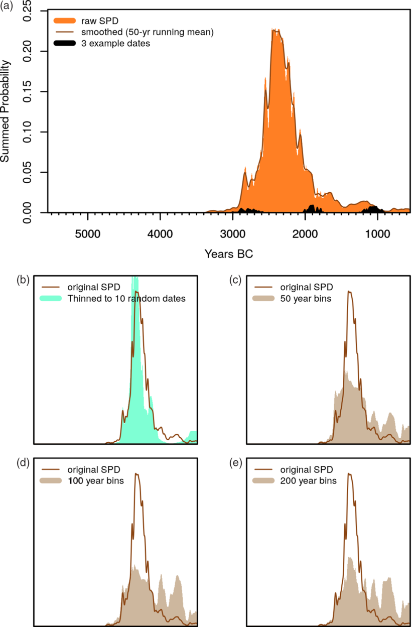
Figure 1 Summing, thinning, and binning: (a) a summed probability distribution of dates from one site only (n = 130 dates), with a slightly smoothed version also shown, as well as three example dates, followed by comparison of the smoothed raw density with (b) a randomly “thinned” dataset of just 10 dates from the same site, (c–e) binned datasets at clustering cut-offs of h = 50, 100 and 200 respectively.
The sharply increasing popularity of SPDs over the last decade or so has rightly also prompted criticism, not only with regard to the overall inferential assumptions behind the idea, but also with respect to the viability of particular SPD-based analytical methods. For example, several researchers have emphasised the fact that the sampling intensity of 14C dates might not be constant over time. A good example is the difference between the popularity of 14C sampling in early Mediterranean prehistory (e.g. Mesolithic-Neolithic) versus its almost complete avoidance for the Greek or Roman periods of the same region, even though the latter was manifestly a period of considerable population (Palmisano et al. Reference Palmisano, Bevan and Shennan2017). In addition to the impact of this differing prioritisation of absolute versus relative dating by archaeologists working on different time periods, researchers have further suggested that different kinds of societies (of otherwise roughly similar population size, for instance) might conceivably produce different 14C footprints and/or that, even if a correlation between dates and population exists, that these might not scale in a linear fashion (Freeman et al. Reference Freeman, Byers, Robinson and Kelly2017). Others have noted that there might be a taphonomic bias towards the preservation of more anthropogenic material from sites of later periods (Surovell and Brantingham Reference Surovell and Brantingham2007; Surovell et al. Reference Surovell, Byrd Finley, Smith, Brantingham and Kelly2009), again implying that over extended periods of thousands of years, we should probably assume a non-linear scaling to human activity. Such critiques are often valid to some degree and focus on how we should interpret summed probability distributions of 14C dates in the first place (see discussions in Contreras and Meadows Reference Contreras and Meadows2014; Mökkönen Reference Mökkönen2014; Tallavara et al. Reference Tallavaara, Pesonen, Oinonen and Seppä2014; Attenbrow and Hiscock Reference Attenbrow and Hiscock2015; Hiscock and Attenbrow Reference Hiscock and Attenbrow2016; Smith Reference Smith2016; Williams and Ulm Reference Williams and Ulm2016) Indeed, some of these very same issues also apply to other attempts to reconstruct past population (e.g. settlement counts where again it is sometimes difficult to compare evenly across periods and regions).
SPDs, however, also face a further challenge at a more fundamental level with regard to how best we might measure the changing frequencies of 14C dates through time. Because calibrated 14C dates comprise probability distributions spread across multiple calendar years and not discrete single estimates, the visual interpretation of aggregated SPDs becomes challenging and very often misleading at multiple scales. Peaks and troughs in SPDs might reflect changes in date intensity through time (and hence interpreted as population “booms” or “busts”), but they might also be a consequence of the changing steepness of the calibration curve, the size of the dates’ associated measurement errors and/or just a statistical fluke from small sample sizes. In response to these challenges, a number of studies (Shennan and Edinborough Reference Shennan and Edinborough2007; Shennan et al. Reference Shennan, Downey, Timpson, Edinborough, Colledge, Kerig, Manning and Thomas2013; Timpson et al. Reference Timpson, Colledge, Crema, Edinborough, Kerig, Manning, Thomas and Shennan2014; Crema et al. Reference Crema, Habu, Kobayashi and Madella2016, Reference Crema, Bevan and Shennan2017; Bevan et al. Reference Bevan, Colledge, Fuller, Fyfe, Shennan and Stevens2017; Bronk Ramsey Reference Bronk Ramsey2017; Brown Reference Brown2017; Edinborough et al. Reference Edinborough, Porčić, Martindale, Brown, Supernant and Ames2017; Freeman et al. Reference Freeman, Baggio, Robinson, Byers, Gayo, Finley, Meyer, Kelly and Anderies2018; McLaughlin Reference McLaughlin2019; Roberts et al. Reference Roberts, Woodbridge, Bevan, Palmisano, Shennan and Asouti2018) have developed new techniques to address some of these issues. Most notably, they have offered new approaches to the problem of discerning genuine fluctuations in the density of 14C dates as opposed to statistical artifacts arising from sampling error, the calibration process or taphonomic histories. Even so, replication and reuse of such methods remains limited, due both to an understandable experimentation across multiple software packages for calibration and statistical analysis (e.g. OxCal, CalPal, and in various forms via the R statistical environment, see Supplementary Figure 1) and to only patchy provision, so far, of transparent and reproducible workflows.
With a view to exploring and alleviating some of these issues, as well as with an eye to an increasing emphasis across archaeology and many other subjects on reproducible research (see Marwick Reference Marwick2017; Marwick et al. Reference Marwick, d’Alpoim Guedes, Barton, Bates, Baxter, Bevan, Bollwerk, Bocinsky, Brughmans, Carter, Conrad, Contreras, Costa, Crema, Daggett, Davies, Drake, Dye, France, Fullagar, Giusti, Graham, Harris, Hawks, Heath, Huffer, Kansa, Kansa, Madsen, Melcher, Negre, Neiman, Opitz, Orton, Przystupa, Raviele, Riel-Salvatore, Riris, Romanowska, Smith, Strupler, Ullah, Van Vlack, Van Valkenburgh, Watrall, Webster, Wells, Winters and Wren2017), we have recently developed rcarbon as an extension package for R (R Core Team 2018), one of the most popular software environments for statistical computing. The rcarbon package provides basic calibration, aggregation, and visualisation functions comparable to those that exist in other software packages, but also offers a suite of further functions for simulation-based statistical analysis of SPDs. This paper will discuss the main features of rcarbon, will highlight technical details and their implications in the creation and analyses of SPDs, and will offer some additional thoughts on the strengths and weakness of SPD-based methods overall.Footnote 1
CALIBRATION AND AGGREGATION
Basic Treatment: Calibration and Summation
In its most basic form, an SPD extends the idea of a plotting a simple histogram of either uncalibrated 14C ages or median calibrated dates to represent changing density of 14C samples over time. Hence, the construction of an SPD involves two steps: (1) 14C dates are calibrated so that for each sample we obtain a distribution of probabilities that the sample in question belongs to a particular calendar year; and (2) all of these per-year probabilities are summed.Footnote 2 The resulting curve thus no longer represents probabilities, but instead is taken as a measure of date intensity. The rationale is thus not dissimilar to intensity-based techniques such as a univariate kernel density estimate (KDE), although with a crucial difference. In the case of KDE, individual kernels associated to each sample have all the same shape defined by the kernel bandwidth, itself mathematically estimated. In contrast, in the case of SPDs, the probability distributions associated with each 14C date have different shapes depending on measurement error and the particularities of the relevant portion of the calibration curve. Consequently, SPDs are not explicitly and straightforwardly an estimate of the underlying distribution from which the observations are sampled from, and its absolute values cannot be directly compared across datasets. It follows that their visual interpretation within and across datasets is intrinsically biased.
Basic calibration in rcarbon is conducted with reference either to one of the established marine or terrestrial calibration curves or to a user-specific custom curve (in what follows, IntCal20 is used throughout: Reimer et al. Reference Reimer, Austin, Bard, Bayliss, Blackwell, Bronk Ramsey, Butzin, Cheng, Edwards, Friedrich, Grootes, Guilderson, Hajdas, Heaton, Hogg, Hughen, Kromer, Manning, Muscheler, Palmer, Pearson, van der Plicht, Reimer, Richards, Scott, Southon, Turney, Wacker, Adolphi, Büntgen, Capano, Fahrni, Fogtmann-Schulz, Friedrich, Köhler, Kudsk, Miyake, Olsen, Reinig, Sakamoto, Sookdeo and Talamo2020). The arithmetic method is for all intents and purposes identical to the the one adopted by OxCal (Bronk Ramsey Reference Bronk Ramsey2008; leaving aside for a moment the more sophisticated Bayesian routines the latter package uses for more complex phase modelling), and very similar to that used by most other calibration software (Weninger et al. Reference Weninger, Clare, Jöris, Jung and Edinborough2015; Parnell Reference Parnell2018). Some of the terminology used by rcarbon’s standard routine has also been made consistent with Bchron, a well-known R package for handling 14C dates and modelling pollen core chronologies and other age-depth relationships (Haslett and Parnell Reference Haslett and Parnell2008; Parnell Reference Parnell2018; see also the clam package; Blaaw Reference Blaauw2019). In rcarbon, the raw data stored for any given calibrated date consists of probability values per calibrated calendar year BP (but convertible to other calendars such as BC/AD), and it is these per-year probabilities that get summed to produce an SPD. For example, Figure 1a shows the result of adding up 130 dates from the Neolithic flint mines of Grimes Graves, Norfolk with three individual dates shown on top (for a full set and and more recent dates from the site, see Healy et al. Reference Healy, Marshall, Bayliss, Cook, Bronk Ramsey, van der Plicht and Dunbar2014). A final point to note is that many studies apply a final ‘smoothing function’ to the SPD (e.g. Kelly et al. Reference Kelly, Surovell, Shuman and Smith2013, Timpson et al. Reference Timpson, Colledge, Crema, Edinborough, Kerig, Manning, Thomas and Shennan2014, Crema et al. Reference Crema, Habu, Kobayashi and Madella2016, etc.), such as a running mean of between 50 and 200 years, to limit possible artifacts resulting from sampling error (but also from the effects of the calibration process) and discourage over-interpretation of the results (in Figure 1a an example with a 50-year running mean is shown). We return to the pros and cons of such smoothing in what follows.
Phase or Site Over-Representation: Thinning and Binning
In most instances, rather than the single site example provided above, an SPD is constructed across a wider region and using more than one site. As a result, there are further potential biases arising from the fact that not all sites (or indeed site phases) may have received equivalent levels of investment in 14C dating. The Neolithic flint mining site of Grimes Graves in southeastern England, for instance, is associated with an unusual number of radiocarbon dates compared to other British prehistoric sites, but such differences do not accurately reflect a site’s relative size or longevity of use. The cumulative effect of these differences in inter-site sampling intensity, and in particular the presence of abnormally high levels of sampling intensity of particular contexts, could thus generate artificial signals in the SPD. While the ideal approach to the problem is to select only samples referring to specific types of events (e.g. the construction of residential features) and control for sampling intensity via Bayesian inference (e.g. using OxCal’s R_Combine function), the use of larger datasets with heterogeneous samples makes this solution unfeasible.
There are two alternative approaches to account for heterogeneity in sampling intensity. The first one involves manually going through a list of 14C dates and choosing only a maximum number of better (e.g. short-lived, low-error) dates per phase or per site. In rcarbon, this thinning approach can also be achieved (in a less attentive but more automatic manner) using the thinDates function which either selects a maximum subset of dates at random or with a mixed approach that allows for some prioritisation of dates with lower errors (Figure 1b). This approach effectively replaces a set of 14C dates referring to the same “event” with a smaller subset with user-defined size and inclusion criteria. As a consequence, the potentially biased contribution to the SPD of events associated with a larger number of 14C dates can be reduced. A second solution to reduce the potential effect of such bias is to aggregate samples from the same site that are close in time, sum their probabilities, and divide the resulting SPD by the number of dates. Such site or phase-level “binning” was introduced by Shennan et al. (Reference Shennan, Downey, Timpson, Edinborough, Colledge, Kerig, Manning and Thomas2013) and discussed in detail by Timpson et al. (Reference Timpson, Colledge, Crema, Edinborough, Kerig, Manning, Thomas and Shennan2014). The rationale is effectively to generate a local SPD referring to a particular occupation phase and to normalize this curve to unity to reduce the impact of heterogeneous sampling intensity. The rcarbon package provides a routine (binPrep), similar but not identical to the ones used in those two discussions, whereby dates from the same sites are grouped based on their (uncalibrated or median calibrated) inter-distances in time, defined by the parameter h, and then put into bins. Dates within the same bins are then aggregated to produce a local SPD that is normalized to sum to unity before being aggregated with other dates (and local SPDs) to produce the final curve.
Different authors have already used different values for h (or comparable parameters) ranging anywhere from 50 to200 years (e.g. Shennan et al. Reference Shennan, Downey, Timpson, Edinborough, Colledge, Kerig, Manning and Thomas2013; Timpson et al. Reference Timpson, Colledge, Crema, Edinborough, Kerig, Manning, Thomas and Shennan2014; Crema et al. Reference Crema, Habu, Kobayashi and Madella2016; Bevan et al. Reference Bevan, Colledge, Fuller, Fyfe, Shennan and Stevens2017; Roberts et al. Reference Roberts, Woodbridge, Bevan, Palmisano, Shennan and Asouti2018). These choices can have a considerable effect on the resulting shape of the within site or within-phase local SPD, with higher values effectively leading to a more spread-out distribution of probabilities (Figures 1c–e) and we recommend exploring the implications of this empirically (e.g. via the binSense routine in rcarbon package (see for example Riris Reference Riris2018). It is also worth noting that there has been little or no discussion on what exactly constitutes a bin (or the “event” on which the thinning procedure is based), and how this might differ as a function of h, and ultimately affect the interpretation of SPDs. For example, bins generated from larger values of h effectively lead to an equal contribution of (potentially differently sized) sites to the SPD, effectively making this a proxy of site density rather than population size.
Normalized vs. Unnormalized Dates
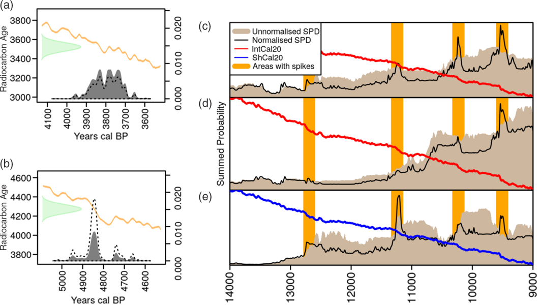
It is well-known that the shapes of individual calibrated probability distributions vary depending on the steepness or flatness of the calibration curve at that point in time. Less well-known is the fact that the area-under-the-curve of a date, calibrated in the usual arithmetic way, will not immediately sum to unity, but instead is typically normalized to ensure that it does (i.e. by dividing by the total sum under the curve for that date). Figures 2a–b provide two examples of dates at flat and steep portions of the calibration curve respectively which produce dramatically different areas-under-the-curve before normalization. Weninger et al. (Reference Weninger, Clare, Jöris, Jung and Edinborough2015) first noted that the presence of this normalizing correction explains the “artificial spikes” noted by several different studies of SPDs, in which such spikes occurred in predictable ways at steep portions of the calibration curve (and which sometimes prompted attempts to smooth them away via fairly aggressive moving averages and/or various forms of kernel density estimate (see Williams Reference Williams2012; Shennan et al. Reference Shennan, Downey, Timpson, Edinborough, Colledge, Kerig, Manning and Thomas2013; Timpson et al. Reference Timpson, Colledge, Crema, Edinborough, Kerig, Manning, Thomas and Shennan2014; Brown Reference Brown2015, Reference Brown2017; Ramsey Reference Bronk Ramsey2017; McLaughlin Reference McLaughlin2019). Figures 2c–e provide three globally wide-ranging examples from the literature of datasets where spikes have been observed, with those spikes being particularly pronounced in early Holocene time series. In contrast, when unnormalized dates are summed, such spikes are not present. On first consideration, it is tempting to deem the normalized dates more theoretically justifiable, regardless of the spikes, because each date is seemingly “treated equally” (i.e. each has a weight of 1 in the summation). However, because the summing a set of unnormalized calibrated dates (with varying post calibration areas under the curve) produces exactly the same result as first summing a set of uncalibrated Gaussians conventional 14C age distributions (each of unity weight) and then calibrating them in one go (the process in CalPal, and also achievable in rcarbon, although not the default: see Supplementary Figure 2), this theoretical premise of the “equal treatment” of each sample (i.e. the issue of unnormalized dates yielding an area under the curve equal to unity) can in fact be argued both ways (see Weninger et al. Reference Weninger, Clare, Jöris, Jung and Edinborough2015 for extensive discussion). Regardless, these issues urge a basic caution not to over-interpret SPD results without considerable attention to how individual highs and lows in the data may have arisen.

Figure 2 Comparisons of unnormalized and normalized dates and their consequences: (a) a single date at a flat portion of the calibration curve (area under the probability histogram: 1.337), (b) a single date at a steep portion of the calibration curve (area under the probability histogram: 0.452), (c) Southern Levantine SPD (ndates = 657, nsites = 119, nbins = 413; data from Roberts et al. Reference Roberts, Woodbridge, Bevan, Palmisano, Shennan and Asouti2018), (d) Sahara SPD (ndates = 643, nsites = 233, nbins = 551; data from Manning and Timpson Reference Manning and Timpson2014), and (e) Brazil SPD (ndates = 173, nsites = 97, nbins = 171; data from Bueno et al. Reference Bueno, Dias and Steele2013).The orange bar highlights time-intervals associated with steeper portions of the IntCal20 (Reimer et al. Reference Reimer, Austin, Bard, Bayliss, Blackwell, Bronk Ramsey, Butzin, Cheng, Edwards, Friedrich, Grootes, Guilderson, Hajdas, Heaton, Hogg, Hughen, Kromer, Manning, Muscheler, Palmer, Pearson, van der Plicht, Reimer, Richards, Scott, Southon, Turney, Wacker, Adolphi, Büntgen, Capano, Fahrni, Fogtmann-Schulz, Friedrich, Köhler, Kudsk, Miyake, Olsen, Reinig, Sakamoto, Sookdeo and Talamo2020) and SHCal20 (Hogg et al. Reference Hogg, Heaton, Hua, Palmer, Turney, Southon, Bayliss, Blackwell, Boswijk, Bronk Ramsey, Pearson, Petchey, Reimer, Reimer and Wacker2020) calibration curves.
STATISTICAL TESTING
While it is tempting to treat the SPD itself as an unproblematic end goal with which to make interpretations about past population dynamics, this is rarely true, and it is almost always important to pay additional analytical attention to a host of uncertainties that come with it. For example, aside from the concerns often voiced about whether the density of 14C dates can be regarded as a reliable proxy (see above), it is also worth noting at least two more issues. First, an ordinary SPD does not depict the uncertainty associated with the fact that certain calendar years are more likely to accrue a more narrowly defined dated sample than others (see Supplementary Figure 3 for a worked through example). Nor does it depict the further uncertainty associated with larger or smaller sample sizes of dates or their measurement errors. A large number of 14C dates for a given study may well improve the chance of a good signal, but there is no magic threshold, as this depends very much on the scope and goals of the analysis (e.g. inferences about multi-millennial trends versus those about sub-millennial trends, inferences about perceived growth rates through time or instead about regional differences across geographic space).
Model Fitting and Hypothesis Testing
There have been various attempts so far to address these uncertainties, most of them leveraging the flexibility of Monte Carlo-type conditional simulation in some fashion, although more formally Bayesian models have also been proposed (see final section). Perhaps the most well-known approach was introduced by Shennan et al. (Reference Shennan, Downey, Timpson, Edinborough, Colledge, Kerig, Manning and Thomas2013) and compares an observed SPD with a theoretical null hypothesis of population change, where the latter might for instance imply stability (e.g. a flat, uniform theoretical SPD), growth (e.g. an exponential theoretical model) or initial growth-and-plateau (e.g. a logistic model) to name just a few of the most common (e.g. Shennan et al. Reference Shennan, Downey, Timpson, Edinborough, Colledge, Kerig, Manning and Thomas2013; Crema et al. Reference Crema, Habu, Kobayashi and Madella2016; Bevan et al. Reference Bevan, Colledge, Fuller, Fyfe, Shennan and Stevens2017, Fernández-López de Pablo et al. Reference Fernández-López de Pablo, Gutiérrez-Roig, Gómez-Puche, McLaughlin, Silva and Lozano2019). The usual workflow involves (1) fitting such a theoretical model to the observed SPD, (2) drawing s dates proportional to the shape of this fitted model (where s matches the number of observed dates or the number of bins if the dates have been binned), (3) back-calibrating individual dates from calendar time to 14C age, and assigning an error to each by randomly sampling (with replacement) the observed 14C age errors in the input data, (4) generating a theoretical SPD from the simulated data obtained in steps 2 and 3, (5) repeating steps 2–4 n times and generating a critical (e.g. 95%) envelope for the theoretical SPD given the sample size, and (6) computing the amount that the observed SPD falls outside the simulation envelope compared to the randomised runs to produce a global p-value (as extensively described by Timpson et al. Reference Timpson, Colledge, Crema, Edinborough, Kerig, Manning, Thomas and Shennan2014). These general steps have separately implemented by several authors (Crema et al. Reference Crema, Habu, Kobayashi and Madella2016; Porčić and Nikolić Reference Porčić and Nikolić2016; Zahid et al. Reference Zahid, Robinson and Kelly2016; Silva and Vander Linden Reference Silva and Vander Linden2017) with some minor differences (e.g. the formula for calculating the p-value, screening for false positives, etc.), and effectively treats the observed SPD as something comparable to a test statistic.
This approach has had the great virtue of grappling with the uncertainties associated with SPDs directly, but it is worth noting nevertheless that the choice, fitting and simulation of a null model of this kind is not straightforward. First, there are non-trivial technical niceties to do with how such a model is fitted in terms of the error model (e.g. log-linear or non-linear), or the time interval over which the model is fitted versus the interval over which it is simulated (given that all SPDs suffer from edge effects at their start and end dates). Second and more importantly, a particular model of theoretical population change or stability has to be selected and justified on contextual grounds, with perhaps the idea of exponential growth carrying the most straightforward demographic assumptions (all other things being equal and in light of the very long-term trend towards higher global population densities that seems to support this), but with other models often providing better fit to data or allowing certain kinds of extrapolation (e.g. Silva and Vander Linden Reference Silva and Vander Linden2017). A final point to stress regards the general limitations associated with the whole null hypothesis-testing approach: with a large enough sample, it will always be possible to produce a “significant” result, but this may not warrant the kind of interpretation archaeologists and others are often looking for (e.g. about population “booms” and “busts”). It is also worth noting that intervals identified as positive or negative deviations from the null model are based on the density of dates and not on the trajectory of growth or decline even though the latter may be more interpretatively relevant in many situations. This means that, for example, intervals with positive deviations might well include instances of a decline in the density of 14C dates. The Monte-Carlo simulation framework can be easily adapted to take this into account, allowing for testing against growth rates (see Supplementary Figure 4). Finally, the 95% critical envelopes produced for assessments of localised departure of the observed SPD from a theoretical pattern or a second SPD (see below, figures 3-4 for examples) are indicators only and should not be read as a set of formal significance tests for all years as this runs the well-known risk of multiple testing (see Loosmore and Ford Reference Loosmore and Ford2006: 1926, for similar issues associated with the Monte Carlo envelopes produced for spatial point pattern analysis).

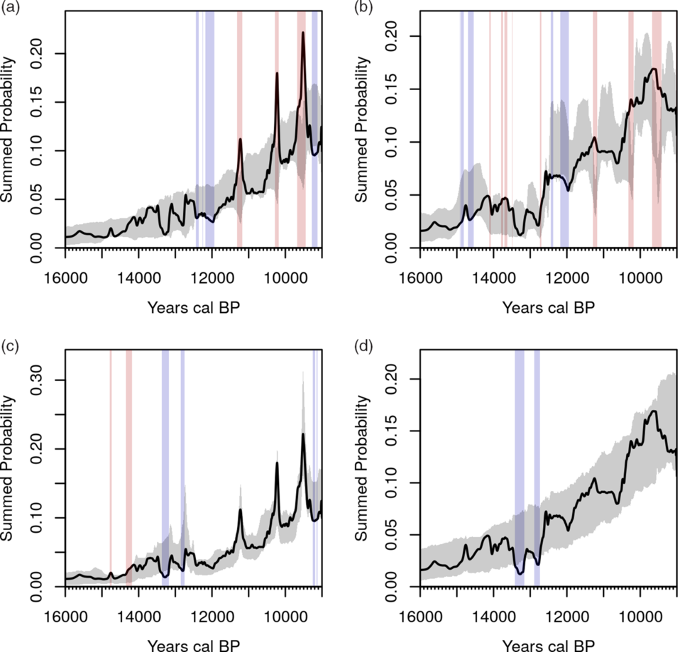
Figure 3 The relationship between observed data and simulations envelopes for four different methods (using the same data as in Figure 2c): calsample realizations of (a) normalized and (b) unnormalized dates, and uncalsample realizations of (c) normalized and (d) unnormalized dates. Temporal ranges highlighted in red and blue represent intervals where the observed SPD show a significant positive or negative deviation from the simulated envelope (they do not necessarily imply the onset point of significant growth or decline).

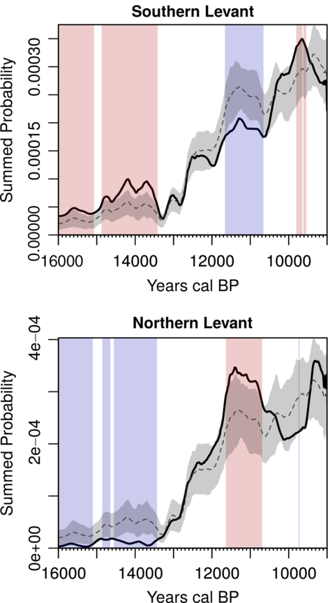
Figure 4 Example of mark permutation test (Crema et al. Reference Crema, Habu, Kobayashi and Madella2016), comparing the SPDs from the Southern (ndates = 657, nsites = 119, nbins = 413) and Northern Levant (ndates = 589, nsites = 41, nbins = 296). Temporal ranges highlighted in red and blue represents intervals where the observed SPD show a significant positive or negative deviation from the pan-regional null model. Data from Roberts et al. (Reference Roberts, Woodbridge, Bevan, Palmisano, Shennan and Asouti2018).
Many existing implementations of this technique both fit and sample from their theoretical models in calendar time. A set of individual calendar years are first drawn proportional to the fitted model, then these are back-calibrated individually to become a set of conventional (uncalibrated) 14C ages with small errors deriving from those associated with the calibration curve itself. Then, larger plausible error terms are added to mimic the instrumental measurement errors of the observed dates and each age (typically now a Gaussian probability distribution) is then calibrated back into calendar time before all of the simulated dates are then finally aggregated into an SPD. This procedure can be formally described by a marginal probability with the assumption of a discretized calendar timeline:
 $$p\left( r \right) = \mathop \sum \nolimits_t^T {\rm{Pr}}\left( t \right)\times p(r|{\mu _t},\sigma _t^2)$$
where p(r) is the probability of selecting a random sample with a 14C age r, Pr(t) is the probability obtained from the fitted theoretical model at the calendar year t within T points in time across the temporal window of analysis, μt and σt are their corresponding date in 14C age and the associated error on the calibration curve, and p(r|μt,σt) refers to the Gaussian probability density function. Thus, if we ignore binning, given an observed dataset with k 14C dates and a theoretical model Pr(t), one could apply Equation (1) to obtain k 14C ages, to which we can assign random instrumental measurement errors by resampling from the observed data.
The term Pr(t) is generally obtained by (1) fitting a curve (via regression) to an observed SPD over a defined temporal window; and (2) transforming the fitted values (e.g. for each discrete calendar year) so they sum to unity. Shennan et al. (Reference Shennan, Downey, Timpson, Edinborough, Colledge, Kerig, Manning and Thomas2013) initially fitted an exponential curve (as a null expectation for population with a constant growth rate), but other models have also been applied subsequently (cf. Crema et al. Reference Crema, Habu, Kobayashi and Madella2016; Bevan et al. Reference Bevan, Colledge, Fuller, Fyfe, Shennan and Stevens2017). It is also worth noting that Pr(t) does not have to be based on observed SPDs and could potentially be derived from theoretical expectations or other demographic proxies (see Crema and Kobayashi Reference Crema and Kobayashi2020 for an example).
The assumption behind this sampling and back-calibration procedure (referred to in rcarbon as the calsample method, due to its sampling in calendar time) is that it will directly emulate both the kinds of uncertainty associated with a given observed sample size, and the impact on an SPD of the non-linearities in the calibration curve itself. However, the relationship between calendar years and 14C ages is not commutative in the way such an approach implies (in agreement with Weninger et al. Reference Weninger, Clare, Jöris, Jung and Edinborough2015), and major problems are encountered in certain narrow parts of the calendar timescale, coincident with the same zones of artificial spiking first described above. Figures 3a–b depict the problem for the later Pleistocene and earlier Holocene time-frame using the same dated as in Figure 2c. As before, we can note the difference in terms of spiking observed at predictable portions of the calibration curve where such spikes are present if we normalize individual dates but absent if we do not. However, the simulated envelopes created by the calsample approach exhibit quite different statistical artifacts at these locations (slight, offset dips if dates are normalized and dramatic dips if they are not). In neither case, do they seem to emulate the observed patterns.
In contrast, one alternative for generating theoretical SPDs is to back-calibrate the entire fitted model in one go and then to weight the result p(r) by the expected probability of sampling r under a uniform model:
 $$v\left( r \right) = {\frac{{\mathop \sum \nolimits_t^T Pr\left( {t|null} \hskip 1pt\right)\times p(r|{\mu _t},\sigma _t^2)}}\over{{\mathop \sum \nolimits_t^T Pr\left( {t|uniform} \right)\times p(r|{\mu _t},\sigma _t^2)}}$$
Here Pr(t|null) is the fitted model under the null hypothesis, and Pr(t|uniform) is the probabilities associated with a uniform distribution covering for the same temporal range T. v(r) is then normalized to unity:
 $$w\left( r \right) = {\frac{{v\left( r \right)}}\over{{\mathop \sum \nolimits_r^R v\left( r \right)}}$$
with R being all the 14C ages examined, most typically the range covered by the calibration curve.
Simulations following this approach then draw samples of uncalibrated ages from the back-calibrated model and calibrate these, before summing (this is therefore referred to in rcarbon as the uncalsample method, see also Roberts et al. Reference Roberts, Woodbridge, Bevan, Palmisano, Shennan and Asouti2018; Bevan et al. Reference Bevan, Colledge, Fuller, Fyfe, Shennan and Stevens2017 for applications). The adjustment of the probability of sampling specific 14C ages according to a baseline uniform model allows for much better simulation of the presence and amplitude of artificial peaks in the SPD at steeper portions of the calibration curve when dates are normalized, and their absence when dates are left unnormalized (Figures 3c–d). However, we note that neither approach is likely to be ideal, and we discuss some promising alternatives in the sections below.
Comparison and Testing of Multiple SPDs
A key advantage of SPDs over more traditional proxies of prehistoric population change, such as settlement counts, is the greater ease with which trajectories across different geographical regions can be compared, without the analytically awkward frameworks imposed by different relative artifact-based chronologies. With this in mind, Crema et al. (Reference Crema, Habu, Kobayashi and Madella2016) developed a permutation-based test to statistically compare two or more SPDs. While the null hypothesis for the one-sample models discussed above is a user-supplied theoretical growth model (e.g. we should expect exponential population growth all other things being equal), the null hypothesis of the multi-sample approach is that the SPDs are samples derived from the same statistical population (e.g. there is no meaningful difference between the shape of the SPD for region A and the one for region B). As for the one-sample approach p-values are obtained via simulation, but in this case rather than generating samples from a theoretical fitted model, the label defining the membership of each date (or bin if binning is being used) is permuted (e.g. we shuffle which dates belong to group A and which ones belong to group B, then produce a new SPD for each group, and repeat many times). This approach can be used to compare SPDs from different regions (as in Crema et al. Reference Crema, Habu, Kobayashi and Madella2016; Bevan et al. Reference Bevan, Colledge, Fuller, Fyfe, Shennan and Stevens2017; Riris Reference Riris2018; Roberts et al. Reference Roberts, Woodbridge, Bevan, Palmisano, Shennan and Asouti2018) in order to infer where local population dynamics differ significantly through time, but it can also be used to consider other groupings of dates, such as those taken on different kinds of physical 14C sample (Bevan et al. Reference Bevan, Colledge, Fuller, Fyfe, Shennan and Stevens2017). Such a mark permutation test will generate simulation envelopes for each SPD whose width proportional to the sample size (i.e. the overall number of dates per region, or the overall number of bins if binning has been applied; Figure 4). Similar to the case of the one-sample approach, both one global and a set of local p-values can be obtained, the former assessing whether there are significant overall differences between sets and the latter identifying particular portions of the SPD with important differences in the summed probabilities.
While there are certainly still ways to mis- or over-interpret the results of this kind of mark permutation test, one major strength is that they do not face quite the same problems associated with model selection, fitting and simulation that the one sample approach does.
SPATIAL ANALYSIS
A regional mark permutation test such as described above already offers one way to compare different geographic regions, but its application requires a crisp definition of these regions from the outset and it is thus not a particularly flexible way to explore variation across continuously varying geographic spaces. Early extensions of the SPD approach already had further spatial inferences in mind when they made use of weighted kernel density estimates (KDE) to infer regions of high or low concentrations of dates across multiple temporal slices, occasionally using animations (e.g. Collard et al. Reference Collard, Edinborough, Shennan and Thomas2010; Manning and Timpson Reference Manning and Timpson2014). Such visual inspection can be the basis for developing specific hypotheses, but suffers from the same limitations as a non-spatial SPDs: it is hard to know what to interpret as interesting variation in date intensity, through time and space, versus variation introduced by the calibration process, by sampling error or by investigative bias. Recent spatio-temporal analyses of 14C dates have tackled this issue in two distinct ways, and we consider each one in turn below.
Flexible Timeslice Mapping
In rcarbon, for instance, it is possible to map the spatio-temporal intensity of observed 14C dates as relevant for a particular “focal” year (using the stkde function). This is achieved by first computing weights associated with each sampling point x given the “focal” year f and temporal bandwidth b using the following equation:
 $$w\left( {x,f,b} \right) = \mathop \sum \nolimits_i^T {p_i}\left( x \right){e^{\frac{{ - {{\left( {i - f} \right)}^2}}}\over{{2{b^2}}}}}$$
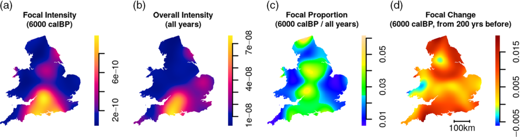
where p i (x) is the probability mass associated with the year i obtained from the calibration process. In other words, a temporal Gaussian kernel is placed around a chosen year and then the degree of overlap between this kernel and the probability distribution of each date is evaluated. Each georeferenced date also has a Gaussian distance-weighted influence on spatial intensity estimate at a given location on the map (with the help of the R package spatstat: Baddeley et al. Reference Baddeley, Rubak and Turner2015): in other words, a spatio-temporal kernel is applied, with both the spatial and the temporal Gaussian bandwidths defined by the user. The choice of appropriate spatial and the temporal bandwidth can arise from data exploration which suggests combinations that are both empirically-useful (e.g. for the particular problem or question of interest) and practically-aware (e.g. of the positional and temporal uncertainties in the underlying data), or it can be made via one of several automatic bandwidth selectors (see Davies et al. Reference Davies, Marshall and Hazelton2018 for a specific review tailored to spatio-temporal analysis). While the latter option has the advantage of avoiding somewhat arbitrary values for the kernel bandwidth, it is worth noting that the choice of different bandwidth selectors can lead to very different result, particularly in the context of spatio-temporal analysis where there is no single agreed algorithm Footnote 3 . Figure 5a shows an example of the resulting surface for the focal year 6000 cal BP, while Figure 5b shows an unchanging overall surface where all samples are treated equally regardless of their actual date (i.e. an ordinary kernel density map).

Figure 5 Example output of one focal year of a kernel density map of English and Welsh dates from the Euroevol Neolithic dataset (ndates = 2327, nsites = 653, nbins = 1461, data from Manning et al. Reference Manning, Colledge, Crema, Shennan and Timpson2016): (a) the spatio-temporal intensity for the focal year 6000 cal BP, (b) the overall spatial intensity for Neolithic dates (8000–4000 cal BP), (c) the proportion of (a) out of (b), and (d) a measure of the spatial pattern of change, mostly growth, from 6200 cal BP to 6000 cal BP.
Figure 5c shows the result of dividing one by the other which offers an indication of the proportion of local dates belonging to the focal, target time period, thereby to some extent detrending for any recovery biases present in the overall sample. This is analogous and consistent with the idea of relative risk mapping (Kelsall and Diggle Reference Kelsall and Diggle1995; Bevan Reference Bevan2012) and such an approach has been used by Chaput et al. (Reference Chaput, Kriesche, Betts, Martindale, Kulik, Schmidt and Gajewski2015) and Bevan et al. (Reference Bevan, Colledge, Fuller, Fyfe, Shennan and Stevens2017) to investigate spatial variation in the 14C density North America and in the British Isles respectively. Figure 5 d shows a further and final useful measure is of “change” between the focal year and some earlier reference or backsight year (e.g. 200 years before, with various options for how “change” or growth/decline is expressed). Color ramps can be standardized to allow comparison across time-slices and thus also animation through multiple timeslices.
Spatial Testing
The above spatial mapping emphasises flexible visualisation, but a complementary second approach to spatial analysis or georeferenced 14C lists instead prioritises the testing of any observed spatial trends, via an extension of the permutation method described above. It compares local SPDs (i.e. SPDs created at each observation point by weighting the 14C contribution of neighboring sites as a function of their distance to the focal point) to the expected local SPD under stationarity (i.e. all local SPD showing the same pattern), obtained via a random permutation of the spatial coordinates of each site. The result (Figure 6) provides a significance test for each site location, highlighting regions with higher or lower growth rates compared to the pan-regional trend (see also Crema et al. Reference Crema, Bevan and Shennan2017).

Figure 6 Spatial permutation test for the same data as Figure 5 showing: (a) the local mean geometric growth rates mean geometric growth rate between 6300–6100 to 6100–5900 cal BP; and (b) results of the spatial permutation test for the same interval showing local significant positive and negative significant departures from the null hypothesis.
CONCLUSION
As the above should make clear, we continue to see great promise in the aggregate treatment of 14C dates as proxies for activity intensity, and it is interesting to note that similar conclusions have been made in other fields that do not focus on human population, but instead use such lists to explore, amongst other things, alluvial accumulation, volcanic activity or peat deposition (Michczyńska and Pazdur Reference Michczyńska and Pazdur2004; Surovell et al. Reference Surovell, Byrd Finley, Smith, Brantingham and Kelly2009; Macklin et al. Reference Macklin, Lewin and Jones2014). The basic notion behind an SPD remains relatively easy to understand and in part this is probably the reason for its widespread appeal, even if some of the ensuing testing methods become more complicated. The rcarbon package is an attempt to provide a working environment within which to explore both the strengths and weaknesses of such an approach. There is also a useful transferability of SPD approaches to proxy time series constructed from other kinds of evidence, such as dendrochronological dates (Ljungqvist et al. Reference Ljungqvist, Tegel, Krusic, Seim, Gschwind, Haneca, Herzig, Heussner, Hofmann, Houbrechts, Kontic, Kyncl, Leuschner, Nicolussi, Perrault, Pfeifer, Schmidhalter, Seifert, Walder, Westphal and Büntgen2018) or even traditionally dated artifact datasets. Even so, there continues to be a real need to consider how alternatives, for example Gaussian mixtures (Parnell Reference Parnell2018), might offer superior and theoretically more coherent frameworks, and to grapple further with quantisation and calibration curve effects (Weninger and Clare Reference Weninger and Clare2018).
ACKNOWLEDGMENTS
We would like to thank several colleagues with whom we have discussed many aspects of this paper, as well those who provided constructive feedback on the rcarbon package, in particular: Anna Bloxam, Kyle Bocinsky, Kevan Edinborough, Martin Hinz, Alessio Palmisano, Phil Riris, Peter Schauer, Fabio Silva, Stephen Shennan, and Bernhard Weninger. We are also grateful to the three anonymous reviewers for their insightful comments on the manuscript. This project has received funding from the European Research Council (ERC) under the Horizon 2020 research and innovation program (Grant Agreement No 801953). This material reflects only the authors’ views and the Commission is not liable for any use that may be made of the information contained therein.
Supplementary material
To view supplementary material for this article, please visit https://doi.org/10.1017/RDC.2020.95


 Open access