


5.1 Introduction
International migration – especially of high-skilled, high-educated people – is on the rise. Accordingly, academic scholars have made efforts and great progress in better understanding the patterns of migration flows across countries and their composition and characteristics – for instance, skills and gender composition. In a similar vein, governments in high-income countries have become increasingly aware of the importance of attracting skilled labor abroad to tackle skills’ shortages and scant entrepreneurial talent. Indeed, research has documented that high-skilled immigrants make a strong contribution to their host economies (see Chapter 6). As a result, many governments have introduced selective immigration policies to increase the inward flows of knowledge workers. On their side, many sending economies – not necessarily only developing countries (EU and OECD 2016) – are struggling to retain their highly trained human capital. Further evidence on what attracts and retains knowledge workers is therefore required.
This chapter contributes to the literature by studying the causes of international migration and, in particular, the determinants of the international mobility of knowledge workers, which is still an underdeveloped research avenue (Brücker et al. Reference Brücker, Facchini, Bertoli, Mayda, Peri, Boeri, Brücker, Docquier and Rapoport2012; Ortega and Peri Reference Ortega and Peri2013). We make use of the original data set on migrant inventors described in detail in Chapter 4 as a proxy for knowledge workers and study their migration patterns over a long period of time. We first investigate whether knowledge migration patterns and trends can be studied within the same framework that has been applied to the international migration of all workers. To achieve this goal, we make use of the well-known gravity model of international migration (for a recent survey, see Beine et al. Reference Beine, Bertoli and Fernández-Huertas Moraga2016).
The theoretical foundations for the gravity approach come from Roy (Reference Roy1951), Sjaastad (Reference Sjaastad1962), and Borjas (Reference Borjas1987, Reference Borjas1989), who all build different models that formalize the decision to migrate as a function of income differentials between origin and destination economies, net of the costs of moving to another country. Recent data availability on a dyadic basis (origin-destination countries) – as commented on in Chapter 2 – has allowed researchers to empirically test these and other ideas and identify the push and pull factors of international migration. Thus research has shown that income differentials between receiving and sending countries positively influence the flow of migrants between countries (Beine et al. Reference Beine, Docquier and Özden2011; Belot and Hatton Reference Belot and Hatton2012; Grogger and Hanson Reference Grogger and Hanson2011; McKenzie and Rapoport Reference McKenzie and Rapoport2010; Ortega and Peri Reference Ortega and Peri2013; Pedersen et al. Reference Pedersen, Pytlikova and Smith2008). It has also shown how migration costs – generally proxied by geographic distance and other related variables – hamper bilateral migration flows, while cultural similarity facilitates these flows. Studies have also analyzed whether international migration is influenced by restrictive migration policies adopted in destination countries, with results being mixed (Clark et al. Reference Clark, Hatton and Williamson2007; Karemera et al. Reference Karemera, Oguledo and Davis2000; Mayda Reference Mayda2010).
In addition, we aim to investigate whether migrant inventors show any particularities that eventually would make them a special class of migrant workers. As Docquier and Rapoport (Reference Docquier and Rapoport2009) argue, there is considerable heterogeneity among skilled workers, and this is worth examining. For instance, recent studies show that a large number of scientists and technologists trained in developing countries – between 30 and 50 percent – actually live in the developed world (Barre et al. Reference Barre, Hernandez, Meyer and Vinck2003; Meyer and Brown Reference Meyer and Brown1999). Similarly, Docquier and Rapoport (Reference Docquier and Rapoport2012) report emigration rates of Ph.D. holders and researchers that are between 2.2 and 5.3 times larger than the average rate for tertiary-educated migrants. This is a distinction with important policy relevance because many countries of the Organization for Economic Cooperation and Development (OECD) have recently facilitated skilled immigration as a response to expected shortages of skilled labor (Chaloff and Lemaître Reference Chaloff and Lemaître2009). The US H-1B visa framework and the EU “Blue Card” initiative constitute clear examples of such a trend. Thus countries increasingly fine-tune their immigration policies to make them more skill selective (Brücker et al. Reference Brücker, Facchini, Bertoli, Mayda, Peri, Boeri, Brücker, Docquier and Rapoport2012).
To some extent, the availability of census data has allowed scholars to study the heterogeneity across migrants’ skills groups under the abovementioned framework. In particular, existing studies have tested whether the incidence of push and pull factors of international migration varies with their skills composition. Such studies can be grouped into three main categories. First, there are those studying whether income differentials or migration barriers positively or negatively select migrants on the basis of their skills. For instance, Beine et al. (Reference Beine, Docquier and Özden2011) find an association of income differentials with positive selection of skilled migrants. Similarly, they also find migration barriers to affect the skill composition of flows; in particular, larger migration costs are associated with higher-skilled migrants, and diaspora networks tend to favor lower-skilled migrants. Bertoli and Fernández-Huertas Moraga (Reference Bertoli and Fernández-Huertas Moraga2012) show that low-skilled migrants are more sensitive to changes in the costs of migration – including legal barriers – than skilled migrants.
A second avenue of research has attempted to shed light on what drives the attraction of knowledge workers. There is evidence that urban areas are more attractive to high-skilled, high-income workers due to their larger supply of amenities – for instance, public and social services, a vibrant cultural scene, and historical sites (Glaeser et al. Reference Glaeser, Kolko and Saiz2001). As income rises with skills, so does the demand for (cultural) amenities. If amenities are normal or superior goods, then inventors may be especially predisposed to move to high-amenity countries. Other studies have also introduced tax revenues as determinants of migration (Pedersen et al. Reference Pedersen, Pytlikova and Smith2008). High taxes and tax revenues might be associated with generous social welfare systems, which may attract immigrants. At the same time, tax revenues may affect the skills composition of immigrant flows because studies have shown that high-skilled, high-income workers such as inventors seek to minimize their tax burden when deciding on their location (Akcigit et al. Reference Akcigit, Baslandze and Stantcheva2016; Kleven et al. Reference Kleven, Landais and Saez2013).
Finally, some studies have employed the gravity framework to study the effects of immigration policies. Broadly speaking, they find that selective immigration policies tend to shift the skill composition of immigrants toward higher-skilled categories (Beine et al. Reference Beine, Docquier and Özden2011; Bertoli and Fernández-Huertas Moraga Reference Bertoli and Fernández-Huertas Moraga2012; Grogger and Hanson Reference Grogger and Hanson2011). These results are consistent with the notion that low-skilled migrants are more sensitive to changes in the costs of migration than skilled migrants. Interestingly, they also find that belonging to the Schengen Agreement, as a proxy for lower migration barriers across European countries, positively affects the migration of skilled workers over nonskilled ones, which seems counterintuitive, because lowering migration barriers should favor the migration of low-skilled workers over high-skilled ones.
However, most of the existing studies make use of skilled migration data sets referring to tertiary-educated migrants without further differentiating specific levels of education and areas of specialization. Indeed, there is hardly any research looking specifically at the international mobility of knowledge workers on a large scale and in comparison with the overall population of workers.1 We intend to fill this gap by making use of our new longitudinal data set on the international mobility of inventors applying for Patent Cooperation Treaty (PCT) patents. Following the existing literature (Agrawal et al. Reference Agrawal, Kapur, McHale and Oettl2011; Kerr Reference Kerr2008), we argue that this new data set characterizes international mobility at the upper tail of the skills’ distribution with unique coverage in terms of country pairs and time.
To summarize our main results, we find that inventors’ migration data can be reasonably used to study the migratory patterns of high-skilled workers. In particular, we find that income maximization drives inventor mobility and that it also shapes the educational mix of immigrants in favor of inventors. In addition, migration costs and amenities favor inward flows of this highly skilled class of workers relative to the general population of migrants.
The rest of this chapter is organized as follows: Section 5.2 presents our research strategy and econometric approach. Section 5.3 briefly describes our database, on which Chapter 4 elaborates in greater detail. Section 5.4 presents our econometric results, and Section 5.5 offers concluding remarks.
5.2 Methods
5.2.1 Empirical Model
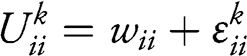
We follow Beine et al. (Reference Beine, Docquier and Özden2011, Reference Beine, Bertoli and Fernández-Huertas Moraga2016) in deriving an empirical model of bilateral migration, starting from a framework of utility maximization set out in previous theoretical work. In particular, in a simplified version of Beine et al. (Reference Beine, Docquier and Özden2011, Reference Beine, Bertoli and Fernández-Huertas Moraga2016), we assume that the utility of an individual k, who originates and lives in country i, is mainly a function of her income wii. Anything else that leads individual k to value the utility of staying in her home country differently from the average of the population residing in i is captured by a stochastic term ( ). Thus
 (5.1)
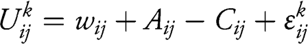
(5.1) Similarly, the utility of individual k, who moves from country i to country j, is a function of her expected income in j(Wij). It also depends on a number of other country-specific factors that may explain her decision to move to j(Aij) – such as amenities or quality-of-life factors – and negatively on the costs incurred when migrating from i to j(Cij). These latter costs consist of information costs, legal barriers, social and cultural differences, and the like. Again, anything else that leads individual k to value the utility of moving to country j differently from the average of the population residing in i is captured by a stochastic term ( ). Thus
 (5.2)
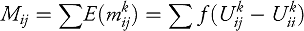
(5.2) If we define a random variable  such that it equals 1 if individual k decides to migrate from i to j and zero otherwise, then the expected gross migration flow from i to j(Mij) would be the sum of the expected values of
  for all k. In addition, we can also express the probability that a random individual from country i will migrate to country j as an increasing function of the difference between the expected utilities of k moving to country j and staying in i:
 (5.3)
(5.3)Assuming that the stochastic terms have a zero mean, we can reformulate Mij as a function of the average income per capita differentials between counties j and i, the migration costs between the two countries, and the factors that may influence positively the decision to move to j:
 (5.4)
(5.4)Following Beine et al. (Reference Beine, Docquier and Özden2011, Reference Beine, Bertoli and Fernández-Huertas Moraga2016) and Feenstra (Reference Feenstra2004), we define F(·) as an exponential function that varies over time t, includes the variables of interest in a linear manner, and also includes a number of additional controls (Zijt) and fixed effects for origin (δi), destination (δj), and time (δt):
 (5.5)
(5.5)In our framework, Mijt will mainly be the flow of inventors from country i to country j at time t, measured exploiting the nationality information contained in PCT patents. However, following the existing international migration literature, international mobility of the whole population will also sometimes be used as Mijt. Note that in order to test the role of income on the international mobility of inventors and overall populations, we have introduced the ratio between income at destination and income at origin as an explanatory variable. By testing the significance of α1, we can directly evaluate whether the income differential between home and host countries matters. We proxy income by countries’ gross domestic product (GDP) per capita. The ratio of the GDPs per capita captures income-differential effects on the expectation that if mean income in the destination exceeds mean income in the origin, all else equal, the incentive to migrate increases.
5.2.2 Econometric Estimation
Gravity model regressions on trade and migration flows typically log-linearize Equation (5.5) and employ ordinary least squares (OLS) and related estimation techniques. However, the international mobility of inventors is a rare phenomenon that translates into a dependent variable with a very large share of zero observations that cannot be logarithmically transformed. The commonly accepted alternative in the literature is the Poisson pseudo–maximum likelihood (PPML) estimation. Coming from the family of count models, it provides a natural way of dealing with the zero migration flows and the extreme skewness of the dependent variable (Cameron and Trivedi Reference Cameron and Trivedi1998; Santos Silva and Tenreyro Reference Santos Silva and Tenreyro2006).
The econometric results presented in the following sections are PPML estimations of variations of Equation (5.5). Since we observe pairs of countries over time, we do the appropriate clustering of standard errors at the pair level. This is important given that country-pair fixed effects were not included in order to identify the effect of time-invariant dyadic variables such as distance or language.2 Moreover, in order to reduce the risk of simultaneity bias, we lag all time-variant explanatory variables by one period.
5.3 Data and Variable Definitions
To measure inventor migration flows, we rely directly on the migratory background information revealed by inventors’ nationality (see Chapter 4) rather than indirectly inferring a possible migration history via the cultural origin of inventors’ names and surnames (see Chapter 3). A first look at the data already provides interesting insights for our study. First, as expected, a handful of OECD countries stand out as the main destinations for migration. Table 5.1 (upper panel) shows the top ten receiving countries for three separate four-year time windows in our sample, where the United States stands out as being the primary receiving country in the three time periods. Germany, the United Kingdom, Switzerland, and other European countries follow at a certain distance. Second, high-income economies are usually the largest senders of migrant inventors – mainly European economies, with China and India gradually taking the first positions in the last period analyzed (Table 5.1, lower panel). Third, and as a consequence of the preceding two, a look at the main migration corridors reveals the prominence of well-established OECD-to-OECD corridors and, to a lesser extent, non-OECD-to-OECD ones but virtually no non-OECD-to-non-OECD ones (Table 5.2). The United States emerges as the most typical destination country, especially in the second period, where only the Germany-Switzerland corridor ranks in the top ten.
Table 5.1 Top Ten Receiving and Sending Countries of Migrant Inventors during Three Four-Year Time Windows
| Country | Inflows 1991–4 | Country | Inflows 1999–2002 | Country | Inflows 2007–10 |
|---|---|---|---|---|---|
| US | 3,590 | US | 33,883 | US | 92,356 |
| Germany | 1,183 | Germany | 5,777 | Germany | 11,766 |
| UK | 945 | UK | 4,500 | Switzerland | 10,419 |
| Switzerland | 879 | Switzerland | 4,285 | UK | 7,289 |
| France | 639 | France | 2,269 | France | 4,349 |
| Australia | 555 | Netherlands | 2,181 | Netherlands | 3,995 |
| Belgium | 385 | Canada | 1,837 | Japan | 3,336 |
| Canada | 383 | Japan | 1,459 | Canada | 3,247 |
| Netherlands | 202 | Australia | 1,430 | Sweden | 2,710 |
| Sweden | 175 | Belgium | 1,201 | Belgium | 2,581 |
| Country | Outflows 1991–4 | Country | Outflows 1999–2002 | Country | Outflows 2007–10 |
|---|---|---|---|---|---|
| UK | 1,651 | China | 9,005 | China | 25,730 |
| Germany | 972 | Germany | 6,880 | India | 19,109 |
| China | 743 | UK | 6,797 | Germany | 14,233 |
| India | 614 | India | 5,633 | UK | 11,205 |
| US | 461 | France | 3,892 | Canada | 9,918 |
| France | 434 | Canada | 3,644 | France | 9,239 |
| Austria | 401 | US | 2,167 | Italy | 4,965 |
| Canada | 348 | Italy | 1,947 | R. of Korea | 4,858 |
| Italy | 321 | Netherlands | 1,831 | Netherlands | 3,800 |
| Netherlands | 312 | Russia | 1,759 | Russia | 3,252 |
| Origin | Destination | Flows 1991–4 | Origin | Destination | Flows 1991–4 |
|---|---|---|---|---|---|
| UK | US | 646 | China | US | 22,216 |
| India | US | 490 | India | US | 17,254 |
| China | US | 456 | Canada | US | 9,033 |
| Germany | Switzerland | 310 | UK | US | 6,469 |
| Austria | Germany | 282 | Germany | US | 4,698 |
| Canada | US | 273 | Germany | Switzerland | 4,101 |
| Germany | US | 194 | R. Korea | US | 4,038 |
| UK | Australia | 186 | France | US | 3,087 |
| Japan | US | 167 | Japan | US | 2,263 |
| UK | Germany | 158 | Russia | US | 1,741 |
On the basis of these stylized facts, we confine our study of the determinants of inventor migration flows to country pairs that include a large number of sending countries (ninety-one) and a more limited number of receiving countries (fifteen) over the period 1991–2010.3
Note also that our empirical approach compares inventor migration flows with overall migration flows, for which we collect the data from the Ortega-Peri data set (Ortega and Peri Reference Ortega and Peri2013).4 This data set provides an unbalanced panel of bilateral migration flows from 1980 to 2006, relying on information from the OECD’s Continuous Reporting System on Migration data (SOPEMI), the United Nations (2005), and the International Migration Database (IMD).
Our dependent variable captures inventor migration flows for annually repeated four-year moving time windows from 1991 to 2010. The explanatory variables are therefore computed from 1990 to 2006. We use GDP per capita in countries i and j to build the main explanatory variable relating to the income differential, that is, the ratio between wijt and wiit. Annual GDP per capita data come from the World Development Indicators of the World Bank. We proxy migration costs Cijt via several dyadic time-invariant variables. These are the log of geographic distance and a set of dummy variables capturing contiguous countries, common language, and common colonial history. They were sourced from the CEPII distance database (Mayer and Zignago Reference Mayer and Zignago2011).5
In order to supplement this analysis, we use a dummy variable capturing whether in relevant years both the sending and receiving countries belong to the European Union and the European Free Trade Association (EFTA) – agreements aimed at dismantling migration barriers.6 Note that in some cases entrance to the European Union did not coincide with the elimination of migration barriers, particularly in the case of the EU enlargement to Eastern European countries in 2004. Moreover, EU receiving countries granted the freedom to migrate on a bilateral basis and not as a block. For instance, with the enlargement of the European Union toward the East, some countries allowed the free movement of workers from the very beginning (Ireland, Sweden, and the United Kingdom), while others applied transitional periods to accept immigrants from the East. We take all these particularities into account in the construction of our dummy variable. Moreover, the variable is not symmetric, given that it might be that country i accepts immigrants from country j earlier than country j accepts migrants from country i. In any case, we expect inventors participating in the EU migration agreement to face lower legal barriers to move between them (“EU treaty”). Note that we build an alternative variable called “EU whole period,” which is a time-invariant dummy valued 1 if the sending and receiving countries belong to the EU treaty at any point in time. The idea is to account for potential anticipation effects of the treaty – that is to say, migration flows occurring due to the expectation of the two countries removing migration barriers between them.
We include two explanatory variables addressing the destination attractiveness for knowledge workers (Ajt). First, we include the share of population living in urban areas of the destination countries. Usually, urban areas are more attractive to high-skilled, high-income workers due to their larger supply of amenities (Glaeser et al. Reference Glaeser, Kolko and Saiz2001). The underlying data come from the UN Educational, Scientific, and Cultural Organization (UNESCO). Second, we include tax revenue as a share of GDP in the destination countries – also sourced from UNESCO.
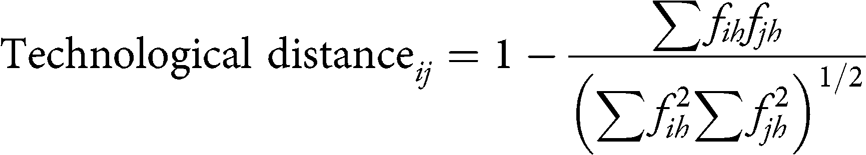
As described in Section 5.2, our estimation also includes a series of additional controls (Zijt). First, we include total bilateral trade – exports plus imports, in logs – as a measure of the intensity of economic linkages between country pairs (ln[EXP + IMP]). Data come from the UN Comtrade Database. Second, we account for the technological distance between countries, as captured by the following index:
 (5.6)
(5.6)where fih stands for the share of patents in country i accounted for by technological class h, and fjh stands for the share of patents in country j accounted for by technological class h.7 Values of the index close to 1 indicate that a given pair of countries is technologically different, and values close to 0 indicate that they are technologically similar (Jaffe Reference Jaffe1986). We use PCT patent data to compute this index.
We further include the number of resident inventors in origin country i and destination country j in order to control for the time-variant underlying geographic distribution of inventors and innovation across the globe – similar to the mass variables in a gravity model. We compute these for moving time windows of five years. Similarly, for the gravity models of overall migration flows, we use total population at the origin and the destination to control for size and the geographic distribution of population over time.
Table 5.3 contains summary statistics of the variables included in the estimations. Concerning our dependent variables, it is interesting to note that the coefficients of variation indicate greater variability in relative terms for inventor migration in our sample than for overall migration – as can be seen directly by the values of the coefficient of variation (CoV). The distance captured by the corridors in our sample range from 80 to 19,500 km. While not centered in this range, the average distance – approximately 4,800 km – can be considered high. This is partially explained by the fact that only 3 percent of corridors in our sample include contiguous countries. In a similar vein, only 12 percent of the corridors correspond to countries sharing the same language, only 4 percent have a past colonial link, and only 4 percent are among two EU or EFTA countries. Both tax revenue and urban population show high values and relatively low variability.
| Variable | Observations | Mean | SD | CoVa | Min | Max |
|---|---|---|---|---|---|---|
| Inventor flows | 20,845 | 56.51 | 533.80 | 9.45 | 0 | 22,216 |
| Population flows | 20,845 | 1,788.32 | 7,477.64 | 4.18 | 0 | 218,822 |
| ln(distance) | 20,845 | 8.40 | 1.01 | 0.12 | 4.39 | 9.88 |
| Contiguity | 20,845 | 0.03 | 0.17 | 5.66 | 0 | 1 |
| Common language | 20,845 | 0.12 | 0.33 | 2.70 | 0 | 1 |
| Colonial links | 20,845 | 0.04 | 0.21 | 4.62 | 0 | 1 |
| Ratio GDP per capita | 20,845 | 6.87 | 9.62 | 1.40 | 0.37 | 84.93 |
| ln(no. of inventors), origin | 20,845 | 4.71 | 3.29 | 0.70 | 0 | 13.34 |
| ln(no. of inventors), destination | 20,845 | 9.26 | 1.51 | 0.16 | 4.09 | 13.34 |
| ln(population), origin | 20,845 | 16.57 | 1.66 | 0.10 | 12.45 | 20.99 |
| ln(population), destination | 20,845 | 16.79 | 1.22 | 0.07 | 15.05 | 19.51 |
| ln(EXP + IMP) | 20,845 | 16.58 | 9.84 | 0.59 | −11.51 | 27.01 |
| Technological distance | 20,845 | 0.45 | 0.29 | 0.64 | 0.02 | 1 |
| EU treaty | 20,845 | 0.05 | 0.23 | 4.20 | 0 | 1 |
| EU whole period | 20,845 | 0.15 | 0.36 | 2.37 | 0 | 1 |
| Tax revenue/GDP, destination | 20,845 | 37.94 | 6.99 | 0.18 | 25.47 | 52.26 |
| Percent population Urban, destination | 20,845 | 78.66 | 8.78 | 0.11 | 61.10 | 97.32 |
a CoV = coefficient of variation.
Table 5.4 presents the correlation matrix for our dependent and independent variables. Given the large sample size, it is not surprising that virtually all Pearson coefficients are significant at 5 percent, and most are so at 1 percent. Of direct interest are the correlations obtained for our two alternative dependent variables. With only two exceptions, both migratory patterns share the same signs, and more important, they behave as expected. The exceptions are GDP per capita at the origin and urban population at destination. The former is expected to be negative but turns out to correlate positively with inventor migration flows. As discussed earlier, this seems less surprising when taking into account that most larger corridors are among OECD countries (see Table 5.2). By contrast, urban population showed a negative correlation for overall migration flows while behaving as expected for inventor migration flows. One explanation may be that overall migration flows include unskilled labor that may be less attracted to amenities than high-skilled labor. Finally, most correlations among explanatory variables are sufficiently low so as to ensure that collinearity does not pose a serious concern. The two main exceptions are the correlations of the origin-country inventors and both technological distance (−0.76) and origin-country GDP per capita (0.72).
Table 5.4 Correlation Matrix
| 1 | 2 | 3 | 4 | 5 | 6 | 7 | 8 | 9 | 10 | 11 | 12 | 13 | 14 | 15 | 16 | 17 | |
|---|---|---|---|---|---|---|---|---|---|---|---|---|---|---|---|---|---|
| 1 | 1 | ||||||||||||||||
| 2 | 0.29 | 1 | |||||||||||||||
| 3 | −0.02 | −0.06 | 1 | ||||||||||||||
| 4 | 0.09 | 0.23 | −0.39 | 1 | |||||||||||||
| 5 | 0.09 | 0.11 | 0.05 | 0.21 | 1 | ||||||||||||
| 6 | 0.04 | 0.14 | 0.04 | 0.08 | 0.37 | 1 | |||||||||||
| 7 | −0.01 | 0.01 | 0.22 | −0.10 | 0.03 | −0.03 | 1 | ||||||||||
| 8 | 0.14 | 0.10 | −0.21 | 0.21 | 0.02 | 0.03 | −0.46 | 1 | |||||||||
| 9 | 0.18 | 0.22 | 0.02 | 0.03 | 0.05 | 0.06 | 0.05 | 0.12 | 1 | ||||||||
| 10 | 0.12 | 0.17 | 0.21 | 0.01 | −0.03 | 0.01 | 0.30 | 0.26 | −0.01 | 1 | |||||||
| 11 | 0.15 | 0.25 | 0.06 | 0.02 | 0.12 | 0.14 | 0.01 | −0.03 | 0.64 | −0.03 | 1 | ||||||
| 12 | 0.08 | 0.09 | −0.04 | 0.10 | 0.06 | 0.06 | −0.21 | 0.44 | 0.21 | 0.16 | 0.08 | 1 | |||||
| 13 | −0.11 | −0.11 | 0.14 | −0.15 | −0.04 | −0.04 | 0.45 | −0.77 | −0.15 | −0.18 | −0.09 | −0.45 | 1 | ||||
| 14 | 0.01 | −0.03 | −0.26 | 0.03 | −0.04 | −0.04 | −0.14 | 0.25 | 0.04 | −0.12 | −0.08 | 0.11 | −0.12 | 1 | |||
| 15 | −0.01 | −0.02 | −0.50 | 0.05 | −0.08 | −0.05 | −0.22 | 0.20 | −0.06 | −0.27 | −0.12 | 0.08 | −0.14 | 0.56 | 1 | ||
| 16 | −0.11 | −0.14 | −0.20 | 0.00 | −0.20 | −0.08 | −0.05 | 0.01 | −0.27 | 0.01 | −0.51 | −0.02 | 0.08 | 0.07 | 0.08 | 1 | |
| 17 | 0.01 | −0.03 | 0.11 | −0.05 | 0.16 | 0.10 | −0.01 | 0.06 | 0.03 | 0.03 | −0.05 | 0.05 | −0.15 | −0.05 | −0.09 | 0.02 | 1 |
Note: 1 = inventors’ flows; 2 = population flows, 3 = ln(distance); 4 = contiguity; 5 = common language; 6 = colonial links; 7 = ratio GDP per capita; 8 = ln(no. of inventors), origin; 9 = ln(no. of inventors), destination; 10 = ln(population), origin; 11 = ln(population), destination; 12 = ln(EXP + IMP); 13 = technological distance; 14 = EU treaty; 15 = EU whole period; 16 = tax revenues/GDP, destination; 17 = percent population urban areas, destination.
5.4 Results
This section presents the estimation results. Table 5.5 shows estimates of the determinants of overall migration and inventor migration from ninety-one sending to fifteen receiving countries by means of PPML (Santos Silva and Tenreyro Reference Santos Silva and Tenreyro2006, Reference Santos Silva and Tenreyro2010). Inventor flows are reported in odd columns and general migrant flows in even columns.
Table 5.5 Determinants of Migration Flows, PPML Estimations, 91 × 15 Sending and Receiving Countries
| Variable | (1) Inventors | (2) All migrants | (3) Inventors | (4) All migrants |
|---|---|---|---|---|
| ln(distance) | −0.549*** | −0.827*** | −0.535*** | −0.814*** |
| (0.0793) | (0.126) | (0.0788) | (0.128) | |
| Contiguity | 0.0742 | 0.348 | 0.100 | 0.332 |
| (0.174) | (0.338) | (0.177) | (0.340) | |
| Common language | 0.874*** | 0.765*** | 0.818*** | 0.759*** |
| (0.145) | (0.189) | (0.139) | (0.191) | |
| Colonial links | −0.0332 | 1.018*** | −0.0158 | 0.996*** |
| (0.142) | (0.202) | (0.142) | (0.207) | |
| Ratio GDP per capita | 0.0975*** | −0.00495 | 0.0965*** | −0.00482 |
| (0.0255) | (0.00563) | (0.0255) | (0.00564) | |
| ln(inventors), origin or ln(population), origin | 0.419*** | 0.339 | 0.408*** | 0.248 |
| (0.0546) | (0.516) | (0.0529) | (0.516) | |
| ln(inventors), destination or ln(population), destination | 0.719*** | 5.602*** | 0.754*** | 5.517*** |
| (0.137) | (1.117) | (0.135) | (1.115) | |
| ln(EXP + IMP) | 0.0231*** | −0.000482 | 0.0217*** | −0.000930 |
| (0.00531) | (0.00432) | (0.00511) | (0.00433) | |
| Technological proximity | −0.241 | −0.396** | −0.227 | −0.395** |
| (0.206) | (0.198) | (0.201) | (0.197) | |
| EU treaty | 0.204* | 0.254 | ||
| (0.110) | (0.183) | |||
| EU whole period | 0.389** | 0.375* | ||
| (0.162) | (0.228) | |||
| Constant | −2.645 | −97.27*** | −8.080*** | −94.23*** |
| (2.227) | (22.98) | (2.690) | (22.62) | |
| Observations | 20,845 | 20,845 | 20,845 | 20,845 |
| Pseudo-R2 | 0.964 | 0.666 | 0.966 | 0.665 |
| Origin-country fixed effects | Yes | Yes | Yes | Yes |
| Destination-country fixed effects | Yes | Yes | Yes | Yes |
| Year fixed effects | Yes | Yes | Yes | Yes |
Note: Robust country-pair clustered standard errors in parentheses.
* p < 0.1; ** p < 0.05; *** p < 0.01.
Our baseline estimation of inventor migration and overall migration flows (columns 1 and 2, respectively) includes the ratio between destination and origin per capita GDP to account for the income differential, the typical variables capturing migration costs – distance in logs, contiguity, common language, and colonial links – and the number of inventors at origin and destination, in order to control for the geographic distribution of inventors and innovation. It also takes into account the strength of economic linkages between country pairs captured by the (log of) bilateral trade and the index of technological distance (Jaffe Reference Jaffe1986). Finally, we include a dummy variable indicating whether sending and receiving countries belong to the European Union and the receiving country does not impose migration barriers to immigrants coming from the origin country in question. Regressions 1 and 2 also include origin, destination, and time fixed effects.
As can be seen from column 1, the per capita GDP ratio positively affects inventors’ flows. Thus larger differences in GDP per capita between the origin and the destination country increase the incentives to migrate. As for the migration cost-related variables, distance has a negative and significant coefficient, in accordance with theory, while contiguity is not significant. Similarly, sharing a common official language influences migration flows positively, but historical links measured as having a common colonial past show no effect with inventor migration as our dependent variable.
In the regression on overall migration flows in column 2, total population at origin and destination replaces the number of inventors at origin and destination used in column 1.8 When comparing inventor flows with population flows, interesting differences emerge. First, all the migration cost variables included seem to affect inventor mobility less than general population mobility. Thus it seems that higher migration costs positively select high-skilled immigrants compared with the general population of migrants. This may be explained by high-skilled migrants being better informed about job opportunities, having better adaptive skills, and being in a better position to handle legal migration barriers. The one exception is the common-language variable, which shows a slightly higher coefficient for inventors. A plausible explanation is that language similarity might be more important for more educated workers because communication is bound to be a prominent factor in high-skilled occupations (Grogger and Hanson Reference Grogger and Hanson2011). The per capita GDP ratio is not significant for overall migration flows, contrary to the case for inventor flows. This finding again points to a skills-biased selection of migrants – this time driven by how skills are rewarded in different locations.
Belonging to the European Union seems to matter only for inventors. This finding seems somewhat counterintuitive because one would expect the elimination of migration barriers to favor the mobility of unskilled labor more than skilled labor. Yet the same results are found in previous studies when comparing the effect of the Schengen Agreement on skilled and unskilled labor flows (Beine et al. Reference Beine, Docquier and Özden2011; Bertoli and Fernández-Huertas Moraga Reference Bertoli and Fernández-Huertas Moraga2012; Grogger and Hanson Reference Grogger and Hanson2011). In any case, the coefficient is only significant at the 10 percent level. In columns 3 and 4, we replace the EU treaty variable with a variable called “EU whole period,” which is a time-invariant dummy valued 1 if the sending and receiving countries belong to the EU treaty at any point in time. The idea is to account for potential anticipation effects of the treaty – that is to say, migration flows occurring due to the expectation of the two countries removing migration barriers between them. As can be seen, the coefficients are considerably larger, significant at 5 percent for the case of inventors and at 10 percent for the general population, possibly confirming the existence of an anticipation effect.
In Table 5.6, we extend the model underlying Table 5.5 by adding additional regressors as possible determinants of inventor migration – both separately and jointly. In particular, we include the tax revenues of the destination countries over GDP and, as a proxy for the supply of cultural amenities, the share of urban population in host economies. As can be seen, the two variables are significant and show the expected sign – note that high taxation seems to harm the attraction of high-skilled workers, as discussed elsewhere (Akcigit et al. Reference Akcigit, Baslandze and Stantcheva2016).9 The even columns in Table 5.6 present the results for overall migration flows. “Tax revenues over GDP” is now positive and significant. This might be explained by the fact that unskilled labor might be more attracted to countries with generous social welfare systems even if those are financed by higher taxes. Finally, the share of urban population by itself exerts a negative influence on overall migration flows, similar to what is shown in the correlation matrix (Table 5.4). However, when we jointly include the taxation and share of urban population variables, the significant effect of the latter disappears. As already pointed out, these variables show low variation across receiving countries and over time, which limits statistical inference – especially in the presence of destination fixed effects.
Table 5.6 Determinants of Migration Flows, PPML Estimations, 91 × 15 Sending and Receiving Countries: Amenities and Tax Revenues
| Variable | (1) Inventors | (2) Population | (3) Inventors | (4) Population | (5) Inventors | (6) Population |
|---|---|---|---|---|---|---|
| ln(distance) | −0.536*** | −0.814*** | −0.535*** | −0.814*** | −0.535*** | −0.814*** |
| (0.0786) | (0.128) | (0.0781) | (0.128) | (0.0781) | (0.128) | |
| Contiguity | 0.102 | 0.332 | 0.104 | 0.332 | 0.104 | 0.332 |
| (0.177) | (0.340) | (0.177) | (0.340) | (0.176) | (0.340) | |
| Common language | 0.817*** | 0.760*** | 0.816*** | 0.760*** | 0.816*** | 0.760*** |
| (0.139) | (0.191) | (0.138) | (0.191) | (0.138) | (0.191) | |
| Colonial links | −0.0129 | 0.994*** | −0.00762 | 0.995*** | −0.00724 | 0.994*** |
| (0.142) | (0.207) | (0.141) | (0.207) | (0.141) | (0.207) | |
| Ratio GDP per capita | 0.0962*** | −0.00483 | 0.0985*** | −0.00471 | 0.0982*** | −0.00483 |
| (0.0250) | (0.00557) | (0.0234) | (0.00558) | (0.0233) | (0.00556) | |
| ln(inventors), origin/ln(population), origin | 0.401*** | 0.240 | 0.388*** | 0.256 | 0.387*** | 0.240 |
| (0.0544) | (0.500) | (0.0569) | (0.505) | (0.0573) | (0.500) | |
| Ln(inventors), destination/ln(population), destination | 0.590*** | 5.078*** | 0.493*** | 7.565*** | 0.453*** | 5.054*** |
| (0.132) | (1.083) | (0.154) | (1.558) | (0.156) | (1.336) | |
| ln(EXP + IMP) | 0.0215*** | −0.000822 | 0.0213*** | −0.000775 | 0.0212*** | −0.000823 |
| (0.00509) | (0.00421) | (0.00490) | (0.00437) | (0.00490) | (0.00421) | |
| Technological proximity | −0.208 | −0.355* | −0.144 | −0.360* | −0.144 | −0.355* |
| (0.207) | (0.192) | (0.196) | (0.196) | (0.199) | (0.193) | |
| EU whole period | 0.388** | 0.375* | 0.384** | 0.375* | 0.384** | 0.375* |
| (0.162) | (0.227) | (0.162) | (0.227) | (0.162) | (0.227) | |
| Tax revenues/GDP, destination | −0.0569*** | 0.0748*** | −0.0245** | 0.0751*** | ||
| (0.0111) | (0.0186) | (0.0124) | (0.0175) | |||
| Percent population urban areas, destination | 0.110*** | −0.0716** | 0.0995*** | 0.000788 | ||
| (0.0255) | (0.0326) | (0.0275) | (0.0286) | |||
| Constant | 0.775 | −87.21*** | −8.873*** | −128.2*** | −6.712*** | −86.80*** |
| (2.220) | (22.25) | (2.276) | (28.99) | (2.591) | (25.34) | |
| Observations | 20,845 | 20,845 | 20,845 | 20,845 | 20,845 | 20,845 |
| Pseudo-R2 | 0.966 | 0.666 | 0.967 | 0.665 | 0.967 | 0.666 |
| Origin-country fixed effects | Yes | Yes | Yes | Yes | Yes | Yes |
| Destination-country fixed effects | Yes | Yes | Yes | Yes | Yes | Yes |
| Year fixed effects | Yes | Yes | Yes | Yes | Yes | Yes |
Note that contrary to the GDP per capita ratio, we were not able to introduce these variables in the model as the relative difference between origin and destination. This is due to insufficient data availability for these variables in origin countries. To address this limitation, we repeat in Table 5A.1 in Appendix 5A the regressions of Table 5.6 with origin fixed effects interacted with time fixed effects. These origin-year fixed effects are aimed at absorbing the effects of tax revenues and the urban population share at the origin, and therefore, it is not necessary to estimate them. Results are comparable to those presented in Table 5.6.
As discussed in our descriptive analysis, there are reasons to believe that determinants of OECD-to-OECD migration flows differ from non-OECD-to-OECD flows. Moreover, the prominence of the United States as a receiving country and China and India as sending countries in our sample also raises some questions about the generality of our results.
The estimations presented in Table 5.7 therefore split our estimation sample according to the origin of migrant flows. In particular, columns 1 through 4 look at migrants coming from other OECD countries, which are mostly high-income economies and we label as “North-North migration.” We again perform separate estimations on both inventor migration and overall migration. Columns 5 through 8 focus on non-OECD origin countries, which we will label as “South-North migration.” Interesting differences emerge with respect to our previous findings. First, we find larger coefficients for the migration cost variables for the South-North case. The strongly negative and large coefficient for the contiguity variable seems somewhat counterintuitive, although we must interpret it with caution, given that only two countries in this sample, Russia and Mexico, observe contiguous flows. The EU variable is not significant in any of the two samples, which we attribute to its low variability within each of the samples. In other words, the EU effect in the preceding regressions is likely to reflect the variation in this variable across the two groups.
Table 5.7 Determinants of Migration Flows, PPML Estimations, 91 ×15 Sending and Receiving Countries: North-North versus South-North Migration
| Variable | (1) | (2) | (3) | (4) | (5) | (6) | (7) | (8) |
|---|---|---|---|---|---|---|---|---|
| OECD origin flows | Non-OECD origin flows | |||||||
| Inventors | Population | Inventors | Population | Inventors | Population | Inventors | Population | |
| ln(distance) | −0.0664 | −0.486*** | −0.0700 | −0.486*** | −1.154*** | −1.382*** | −1.138*** | −1.382*** |
| (0.112) | (0.167) | (0.112) | (0.167) | (0.179) | (0.147) | (0.176) | (0.147) | |
| Contiguity | 0.178 | −0.0377 | 0.178 | −0.0379 | −1.543*** | 2.387*** | −1.539*** | 2.387*** |
| (0.127) | (0.215) | (0.127) | (0.215) | (0.365) | (0.414) | (0.360) | (0.414) | |
| Common language | 0.554*** | 0.796*** | 0.558*** | 0.797*** | 1.199*** | 1.326*** | 1.185*** | 1.326*** |
| (0.108) | (0.215) | (0.109) | (0.215) | (0.209) | (0.192) | (0.207) | (0.192) | |
| Colonial links | 0.0966 | 1.001*** | 0.0997 | 1.001*** | 0.287 | 1.445*** | 0.294 | 1.445*** |
| (0.0959) | (0.245) | (0.0961) | (0.245) | (0.485) | (0.301) | (0.483) | (0.301) | |
| Ratio GDP per capita | 0.195** | 0.0491 | 0.174* | 0.0509 | 0.0277** | −0.00596 | 0.0297** | −0.00595 |
| (0.0973) | (0.0800) | (0.0896) | (0.0806) | (0.0135) | (0.00390) | (0.0126) | (0.00388) | |
| INV/POP, origin | 0.389*** | −2.386** | 0.383*** | −2.406** | 0.150*** | −0.799 | 0.142*** | −0.800 |
| (0.106) | (1.177) | (0.0973) | (1.179) | (0.0227) | (0.602) | (0.0272) | (0.601) | |
| INV/POP, destination | 0.423*** | 5.278*** | 0.350** | 5.778*** | 1.016*** | 4.396** | 0.599** | 5.264*** |
| (0.124) | (1.541) | (0.146) | (1.694) | (0.218) | (1.711) | (0.236) | (1.829) | |
| EU whole period | −0.180 | −0.343 | −0.182 | −0.343 | 0.427 | 0.107 | 0.427 | 0.107 |
| (0.129) | (0.222) | (0.129) | (0.222) | (0.283) | (0.671) | (0.283) | (0.671) | |
| Tax/GDP destination | −0.0447*** | 0.0270 | −0.0239 | 0.0199 | −0.0698*** | 0.124*** | −0.0366*** | 0.115*** |
| (0.0142) | (0.0220) | (0.0152) | (0.0230) | (0.0118) | (0.0249) | (0.0136) | (0.0223) | |
| Percent urban population, destination | 0.0589** | −0.0169 | 0.166*** | −0.0280 | ||||
| (0.0290) | (0.0343) | (0.0370) | (0.0415) | |||||
| Constant | −14.32*** | −28.11 | −20.35*** | −35.07 | 1.128 | −62.43* | −7.750*** | −76.87** |
| (5.023) | (34.16) | (5.366) | (34.60) | (2.843) | (34.17) | (2.848) | (34.69) | |
| Other controls | Yes | Yes | Yes | Yes | Yes | Yes | Yes | Yes |
| Observations | 7,299 | 7,299 | 7,299 | 7,299 | 13,546 | 13,546 | 13,546 | 13,546 |
| Pseudo-R2 | 0.966 | 0.802 | 0.967 | 0.802 | 0.996 | 0.805 | 0.997 | 0.805 |
| Origin fixed effects | Yes | Yes | Yes | Yes | Yes | Yes | Yes | Yes |
| Destination fixed effects | Yes | Yes | Yes | Yes | Yes | Yes | Yes | Yes |
| Year fixed effects | Yes | Yes | Yes | Yes | Yes | Yes | Yes | Yes |
The GDP per capita ratio is significantly larger for the North-North sample. This result is somewhat counterintuitive because one would expect larger income differentials to affect inventor migration more intensively – as suggested in Table 5.5. This may indicate nonlinearities in the relationship between income differentials and inventor migration flows: with moderate income differentials, such as the ones characterizing intra-OECD flows (average GDP ratio = 1.32), they strongly shape the international mobility of knowledge workers. With very large income differentials, such as the ones characterizing non-OECD-to-OECD flows (average GDP ratio = 9.86), the effect of income differentials on migration is more nuanced.10
Finally, Table 5.8 reruns the main models excluding the United States as both a sending and a receiving country (columns 1 and 4), China and India (columns 2 and 5), and the United States, China, and India (columns 3 and 6). Most results and conclusions hold. Interestingly, it seems that the relationship between inventor migration and economic incentives was entirely governed by the excluded countries. Similar results are found for the share of urban population and tax revenues for the case of inventors when we exclude the United States from the analysis, attesting to the importance of this country as a magnet for migrating inventor.11 Further research needs to investigate this point in greater detail.
Table 5.8 Determinants of Migration Flows, PPML Estimations, 91 × 15 Sending and Receiving Countries: North-North versus South-North Migration, without the United States, China, and India
| (1) | (2) | (3) | (4) | (5) | (6) | |
|---|---|---|---|---|---|---|
| Inventors | Population | |||||
| No US | No China, no India | No US, no China, no India | No US | No China, no India | No US, no China, no India | |
| ln(distance) | −0.396*** | −0.441*** | −0.405*** | −0.980*** | −0.917*** | −0.917*** |
| (0.0668) | (0.0607) | (0.0682) | (0.124) | (0.113) | (0.113) | |
| Contiguity | 0.153 | 0.223 | 0.0821 | −0.347 | −0.359 | −0.359 |
| (0.128) | (0.143) | (0.124) | (0.234) | (0.223) | (0.223) | |
| Common language | 1.048*** | 0.703*** | 1.076*** | 1.107*** | 1.127*** | 1.127*** |
| (0.137) | (0.116) | (0.139) | (0.177) | (0.174) | (0.174) | |
| Colonial links | 0.248* | 0.173 | 0.362*** | 1.574*** | 1.589*** | 1.589*** |
| (0.137) | (0.110) | (0.130) | (0.237) | (0.233) | (0.233) | |
| Ratio GDP per capita | 0.0145 | 0.0117 | −0.00200 | −0.00960 | −0.00106 | −0.00106 |
| (0.0113) | (0.0116) | (0.00623) | (0.00919) | (0.0111) | (0.0111) | |
| ln(inventors), origin/ln(population), origin | 0.132*** | 0.274*** | 0.167*** | −0.289 | −0.501 | −0.501 |
| (0.0381) | (0.0599) | (0.0468) | (0.612) | (0.626) | (0.626) | |
| ln(inventors), destination/ln(population), destination | 0.391*** | 0.369*** | 0.376*** | 6.239*** | 6.308*** | 6.308*** |
| (0.112) | (0.136) | (0.114) | (1.697) | (1.926) | (1.926) | |
| ln(EXP + IMP) | 0.0153*** | 0.0148*** | 0.0161*** | 0.000516 | −1.50e−06 | −1.50e−06 |
| (0.00576) | (0.00365) | (0.00572) | (0.00555) | (0.00538) | (0.00538) | |
| Technological proximity | 0.314 | −0.121 | 0.490* | −0.479* | −0.535** | −0.535** |
| (0.250) | (0.196) | (0.268) | (0.254) | (0.266) | (0.266) | |
| EU whole period | −0.0144 | 0.148 | −0.0572 | 0.379 | 0.295 | 0.295 |
| (0.127) | (0.135) | (0.125) | (0.238) | (0.239) | (0.239) | |
| Tax revenues/GDP, destination | −0.0171 | −0.0254** | −0.0165 | 0.120*** | 0.122*** | 0.122*** |
| (0.0185) | (0.0127) | (0.0191) | (0.0208) | (0.0221) | (0.0221) | |
| Percent population urban areas, destination | 0.0127 | 0.0793*** | 0.0123 | 0.0819*** | 0.0817** | 0.0817** |
| (0.0233) | (0.0269) | (0.0239) | (0.0309) | (0.0323) | (0.0323) | |
| Constant | −0.403 | −7.732*** | 1.189 | −85.54*** | −98.54*** | −98.54*** |
| (2.198) | (2.979) | (3.119) | (26.32) | (34.03) | (34.03) | |
| Observations | 19,117 | 20,335 | 18,641 | 19,165 | 18,689 | 18,689 |
| Pseudo-R2 | 0.879 | 0.955 | 0.886 | 0.671 | 0.691 | 0.691 |
| Origin-country fixed effects | Yes | Yes | Yes | Yes | Yes | Yes |
| Destination-country fixed effects | Yes | Yes | Yes | Yes | Yes | Yes |
| Year fixed effects | Yes | Yes | Yes | Yes | Yes | Yes |
5.5 Conclusion
In this chapter we have compiled, used, and evaluated a new database on the international mobility of inventors, spanning a considerable range of years and for a large number of sending and receiving countries. Aside from the methodological improvement of collecting migration information for a larger number of countries and in a longitudinal framework, our database enables us to focus on a specific class of high-skilled individuals. As argued previously, the tertiary-educated labor force is highly heterogeneous. One should expect its movements to imply deeply heterogeneous outcomes as well. We report first econometric results on the importance of typical migration cost and economic incentive variables to explain the migration patterns of inventors. By separately estimating the effect of these variables for inventor migration as well as overall migration flows, we provide evidence on what determines skill selection in international migration.
As a general first conclusion, we firmly believe that aggregated inventor migration data retrieved from patent documents hold substantial promise for studying the migration patterns of this high-skilled class of workers. Most of our results accord with inherited theory and intuitive expectations about what may explain inventor migration, with only few exceptions. Thus, for instance, results point to the importance of economic incentives for attracting and retaining talent. Finally, it appears that higher migration costs tend to positively select skilled immigrants, with the notable exception of language barriers.
Of course, there is still so much to learn about what determines the international movements of knowledge workers. In particular, the paramount role of the United States in explaining the migratory patterns of inventor – and general population – migration needs deeper investigation. Exploiting the information presented here could yield interesting results to understand not only what drives the international mobility of inventors and the global competition for talent but also the relationship of this phenomenon with innovation outcomes in receiving countries, economic development in sending countries, and the international diffusion of ideas.
Table 5A.1 Determinants of Migration Flows, PPML Estimations, 91 ×15 Sending and Receiving Countries: Amenities and Tax Revenues, with Origin × Time Fixed Effects
| Variable | (1) Inventors | (2) Population | (3) Inventors | (4) Population | (5) Inventors | (6) Population |
|---|---|---|---|---|---|---|
| Ratio GDP per capita | 0.341*** | 0.0945*** | 0.339*** | 0.0950*** | 0.338*** | 0.0950*** |
| (0.0409) | (0.0231) | (0.0407) | (0.0231) | (0.0406) | (0.0231) | |
| ln(inventors), destination/ln(population), destination | 0.542*** | 4.211*** | 0.521*** | 7.536*** | 0.467*** | 5.216*** |
| (0.115) | (1.276) | (0.128) | (1.373) | (0.128) | (1.257) | |
| Tax revenues/GDP, destination | −0.0526*** | 0.0809*** | −0.0337*** | 0.0682*** | ||
| (0.0104) | (0.0169) | (0.0107) | (0.0182) | |||
| Percent population urban areas, destination | 0.0735*** | −0.101*** | 0.0582*** | −0.0337 | ||
| (0.0179) | (0.0309) | (0.0189) | (0.0323) | |||
| Constant | −11.26*** | −73.44*** | −21.54*** | −113.8*** | −18.20*** | −84.99*** |
| (2.145) | (20.19) | (2.473) | (21.03) | (2.671) | (19.58) | |
| Other controls | Yes | Yes | Yes | Yes | Yes | Yes |
| Observations | 20,691 | 20,622 | 20,622 | 20,622 | 20,622 | 20,622 |
| Pseudo-R2 | 0.988 | 0.759 | 0.988 | 0.759 | 0.988 | 0.760 |
| Origin-country fixed effects | No | No | No | No | No | No |
| Destination-country fixed effects | Yes | Yes | Yes | Yes | Yes | Yes |
| Origin fixed effects × year fixed effects | Yes | Yes | Yes | Yes | Yes | Yes |
| Year fixed effects | Yes | Yes | Yes | Yes | Yes | Yes |
Note: Robust country-pair clustered standard errors in parentheses.
* p < 0.1; ** p < 0.05; *** p < 0.01.


