2.1. Governing equations

In the current study we make use of the filtered Navier–Stokes equations with Boussinesq approximation coupled with a transport equation for the potential temperature to investigate the flow in and around a large-scale wind farm (Allaerts & Meyers Reference Allaerts and Meyers2017). Such equations read as

(2.1)$$\begin{gather} \frac{\partial \tilde{u}_i}{\partial x_i} = 0, \end{gather}$$

(2.2)$$\begin{gather}\frac{\partial \tilde{u}_i}{\partial t} + \frac{\partial}{\partial x_j} (\tilde{u}_j \tilde{u}_i ) = f_c \epsilon_{ij3} \tilde{u}_j + \delta_{i3} g \frac{\tilde{\theta}-\theta_0}{\theta_0} - \frac{\partial \tau_{ij}^{sgs}}{\partial x_j} - \frac{1}{\rho_0} \frac{\partial \tilde{p}^\ast}{\partial x_i} - \frac{1}{\rho_0} \frac{\partial p_\infty}{\partial x_i} + f_i^{tot}, \end{gather}$$

(2.3)$$\begin{gather}\frac{\partial \tilde{\theta}}{\partial t} + \frac{\partial }{\partial x_j} ( \tilde{u}_j \tilde{\theta} ) =- \frac{\partial q_j^{sgs}}{\partial x_j}, \end{gather}$$

where the horizontal directions are denoted with $i=1,2$ while the vertical one is indicated by $i=3$. Moreover, $\delta _{ij}$ denotes the Kronecker delta while $\epsilon _{ijk}$ is the Levi–Civita symbol. The filtered velocity and potential-temperature fields are noted with $\tilde {u}_i$ and $\tilde {\theta }$, respectively.

The first term on the right-hand side represents the Coriolis force due to planetary rotation, where the frequency $f_c = 2 \varOmega _E \sin \phi$, with $\varOmega _E$ the Earth angular velocity and $\phi$ the Earth latitude. The second component of the angular velocity vector $\varOmega _E \cos \phi$ is neglected here since it is negligible when compared with the other terms in the momentum equations (Wyngaard Reference Wyngaard2010). Thermal buoyancy is taken into account by the second term, where $g=9.81\ {\rm m}\ {\rm s}^{-2}$ denotes the gravitational constant and $\theta _0$ is a reference potential temperature. Moreover, we make use of the Boussinesq approximation so that the incompressible continuity equation holds. This assumption has two implications. First, fluctuations in density are related to thermal effects rather than pressure ones, so that acoustic waves are filtered out. Second, all density variations from the background state are neglected except for the buoyancy term. Consequently, the thermodynamic equation has a direct influence only on the vertical momentum equation. This is a valid assumption for our study since the scale of the vertical motions is much smaller than the density scale height, which is typically in the order of 7 km (Spiegel & Veronis Reference Spiegel and Veronis1960; Allaerts Reference Allaerts2016). Moreover, Maas (Reference Maas2022) performed two wind-farm–LES, one with Boussinesq approximation and one with the anelastic assumption. He found nearly identical numerical results at turbine hub height, with only minor differences several kilometres above the ABL.

The flow is driven across the domain by applying a steady background pressure gradient $\partial p_\infty / \partial x_i$, with $i=1,2$. The latter is related to the geostrophic wind $G$ through the geostrophic balance, where $\rho _0$ denotes a reference air density. The pressure oscillations around $p_\infty$ are denoted with $\tilde {p}^\ast$. Moreover, the term $f_i^{tot} = f_i + f_i^{ra} + f_i^{fr}$ groups all external forces exerted on the flow. Here, $f_i^{ra}$ and $f_i^{fr}$ represent the body forces applied within the RDL and fringe region, respectively, while $f_i$ denotes the wind-turbine drag force. Finally, the effects of unresolved scales are modelled by the subgrid-scale stress tensor $\tau _{ij}^{sgs}$ and the subgrid-scale heat flux $q_j^{sgs}$. The notations $(x_1,x_2,x_3)$ and $(x,y,z)$, $(\tilde {u}_1,\tilde {u}_2,\tilde {u}_3)$ and $(\tilde {u},\tilde {v},\tilde {w})$ and $\tilde {p}^\ast$ and $\tilde {p}$ are used interchangeably. Moreover, for the sake of simplicity, the tilde will not be used in the rest of the article.

2.2. Flow solver

The governing equations (2.1)–(2.3) are solved using the SP-Wind solver, an in-house software developed over the past 15 years at KU Leuven (Meyers & Sagaut Reference Meyers and Sagaut2007; Calaf et al. Reference Calaf, Meneveau and Meyers2010; Goit & Meyers Reference Goit and Meyers2015; Allaerts & Meyers Reference Allaerts and Meyers2017, Reference Allaerts and Meyers2018; Munters & Meyers Reference Munters and Meyers2018; Lanzilao & Meyers Reference Lanzilao and Meyers2022, Reference Lanzilao and Meyers2023b). The solver structure adopted here is mainly based on the version developed and used in Allaerts & Meyers (Reference Allaerts and Meyers2017) and Lanzilao & Meyers (Reference Lanzilao and Meyers2022, Reference Lanzilao and Meyers2023b). The equations are advanced in time using a classic fourth-order Runge–Kutta scheme with a time step based on a Courant–Friedrichs–Lewy number of $0.4$. The streamwise ($x$) and spanwise ($\kern0.7pt y$) directions are discretized with a Fourier pseudo-spectral method. This implies that all linear terms are discretized in the spectral domain while nonlinear operations are computed in the physical domain, reducing the cost of convolutions from quadratic to log-linear (Fornberg Reference Fornberg1996). Furthermore, the 3/2 dealiasing technique proposed by Canuto et al. (Reference Canuto, Hussaini, Quarteroni and Zang1988) is adopted to avoid aliasing error. For the vertical dimension ($z$), an energy-preserving fourth-order finite difference scheme is adopted (Verstappen & Veldman Reference Verstappen and Veldman2003). The effects of subgrid-scale motions on the resolved flow are taken into account with the stability-dependent Smagorinsky model proposed by Stevens, Moeng & Sullivan (Reference Stevens, Moeng and Sullivan2000) with Smagorinsky coefficient set to $C_s=0.14$, similarly to previous studies performed with SP-Wind (Goit & Meyers Reference Goit and Meyers2015; Allaerts & Meyers Reference Allaerts and Meyers2017; Munters & Meyers Reference Munters and Meyers2018). The constant $C_s$ is damped near the wall by using the damping function proposed by Mason & Thomson (Reference Mason and Thomson1992). Furthermore, continuity is enforced by solving the Poisson equation during every stage of the Runge–Kutta scheme. In regard to the turbine trust force, we model it using a non-rotating actuator disk model (Allaerts & Meyers Reference Allaerts and Meyers2015; Goit & Meyers Reference Goit and Meyers2015). We refer to Delport (Reference Delport2010) for more details on the discretization of the continuity and momentum equations while the implementation of the thermodynamic equation and sub-grid scale (SGS) model are explained in detail in Allaerts (Reference Allaerts2016).

2.3. Boundary conditions

The effect of the bottom wall on the flow is modelled with classic Monin–Obukhov similarity theory for neutral boundary layers (NBLs) (Moeng Reference Moeng1984). This wall-stress boundary condition is only dependent on the surface roughness $z_0$, which we assume to be constant. We refer to Allaerts (Reference Allaerts2016) for further details on the implementation. Periodic boundary conditions are naturally imposed at the streamwise and spanwise sides of the computational domain. At the top of the domain, a rigid-lid condition is used, which implies zero shear stress and vertical velocity and a fixed potential temperature. However, in case of stratified free atmospheres, a rigid-lid condition reflects back gravity waves triggered by the wind-farm drag force. To minimize gravity-wave reflection, we adopt a RDL in the upper part of the domain (Klemp & Lilly Reference Klemp and Lilly1977; Durran & Klemp Reference Durran and Klemp1983; Allaerts & Meyers Reference Allaerts and Meyers2017; Lanzilao & Meyers Reference Lanzilao and Meyers2023b). This body force dissipates the upward energy transported by gravity waves before it reaches the top of the domain and it reads as

(2.4)\begin{equation} f_i^{ra} (\boldsymbol{x}) =- \nu(z) \left( u_i(\boldsymbol{x}) - U_{G,i} \right)\!, \end{equation}

where $U_{G,1} = G \cos \alpha$, $U_{G,2} = G \sin \alpha$ and $U_{G,3} = 0$ with $\alpha$ the geostrophic wind angle. Moreover, $\nu (z)$ is a one-dimensional function which reads as

(2.5)\begin{equation} \nu(z) = \nu^{ra} N \left[1 - \cos{\left( \frac{\rm \pi}{s^{ra}} \frac{z - \left(L_z-L_z^{ra} \right)}{L_z^{ra}}\right)} \right]\!, \end{equation}

where $L_z$ and $L_z^{ra}$ denote the height of the computational domain and of the RDL, respectively, while $N = \sqrt {g \varGamma / \theta _0}$ represents the Brunt–Väisälä frequency, with $\varGamma$ the lapse rate in the free atmosphere. Moreover, $\nu ^{ra}$ controls the force magnitude while $s^{ra}$ regulates the function gradient along the vertical direction. Lanzilao & Meyers (Reference Lanzilao and Meyers2023b) have shown that the quality of the RDL strongly depends on these two tuning parameters, which are carefully tuned with the aim of minimizing gravity-wave reflection; see § 2.4.

The periodic boundary condition along the streamwise direction recycles back the wind-farm wake. To break the periodicity and impose an inflow condition, we use a fringe technique (Spalart & Watmuff Reference Spalart and Watmuff1993; Lundbladh et al. Reference Lundbladh, Berlin, Skote, Hildings, Choi, Kim and Henningson1999; Nordstrom, Nordin & Henningson Reference Nordstrom, Nordin and Henningson1999; Inoue, Matheou & Teixeira Reference Inoue, Matheou and Teixeira2014; Stevens et al. Reference Stevens, Graham and Meneveau2014b; Munters, Meneveau & Meyers Reference Munters, Meneveau and Meyers2016; Lanzilao & Meyers Reference Lanzilao and Meyers2023b). This body force reads as

(2.6)\begin{equation} f_i^{fr}(\boldsymbol{x}) =-h(x) \left( u_i(\boldsymbol{x}) - u_{{prec},i}(\boldsymbol{x})\right)\!, \end{equation}

where $u_{{prec},i}(\boldsymbol {x})$ denotes the statistically steady inflow fields provided by a precursor simulation. Moreover, $h(x)$ is a one-dimensional non-negative function that is non-zero only within the fringe region, and is expressed as

(2.7)\begin{equation} h(x) = h_{max} \left[ F\left( \frac{x-x_s^h}{\delta_s^h}\right) - F\left( \frac{x-x_e^h}{\delta_e^h} +1\right) \right] \end{equation}

with

(2.8)\begin{equation} F(x) = \begin{cases} 0 & \text{if } x \leq 0, \\ \dfrac{1}{1+\text{exp}\left( \dfrac{1}{x-1} + \dfrac{1}{x}\right)} & \text{if } 0< x<1, \\ 1 & \text{if } x \geq 1. \end{cases} \end{equation}

The parameters $x_s^h$ and $x_e^h$ denote the start and end of the fringe function support while its smoothness is regulated by $\delta _s^h$ and $\delta _e^h$. Moreover, $h_{max}$ denotes the maximum value of the fringe function.

Lanzilao & Meyers (Reference Lanzilao and Meyers2023b) noted that the standard fringe technique triggers spurious gravity waves that propagate through the domain of interest, significantly altering the numerical results. Therefore, in the current study we use the new wave-free fringe-region technique developed by Lanzilao & Meyers (Reference Lanzilao and Meyers2023b). In addition to applying the body force $f_i^{fr}$ described above, this technique also damps the convective term in the vertical momentum equation within the fringe region, multiplying it by the following damping function:

(2.9)\begin{equation} d(x,z) = 1 - \left[ F\left( \frac{x-x_s^d}{\delta_s^d}\right) - F\left( \frac{x-x_e^d}{\delta_e^d} +1\right) \right] \mathcal{H}(z-H). \end{equation}

Here, $x_s^d$ and $x_e^d$ define the start and end of the damping function support while $\delta _s^d$ and $\delta _e^d$ control the function smoothness. Moreover, $H$ denotes the capping-inversion height while $\mathcal {H}$ represents a Heaviside function. For more details, we refer the reader to Lanzilao & Meyers (Reference Lanzilao and Meyers2023b) and to § 2.4 below.

2.4. Numerical set-up

The flow solver makes use of two numerical domains concurrently marched in time, i.e. the precursor and main domains. The precursor domain does not contain turbines and is only used for generating a turbulent fully developed statistically steady flow that drives the simulation in the main domain. Similarly to Allaerts & Meyers (Reference Allaerts and Meyers2017, Reference Allaerts and Meyers2018), we fix the precursor domain length and width to $L_x^p=L_y^p=10$ km, with $L_z^p=3$ km. The wind farm is located in the main domain. The first-row turbine should be far enough from the inflow to properly capture the flow slow down in the farm induction region. Moreover, the last-row turbine should be far enough from the fringe region to minimize spurious effects and to let the farm wake to develop. Similarly, the domain width should be large enough to minimize sidewise blockage and to limit the channelling effects at the farm sides. In Appendix A we present an extensive domain sensitivity study, where we analyse in detail the effects of the domain size on the numerical results. Based on this, we select a domain size of $L_x \times L_y = 50 \times 30\ {\rm km}^2$, with a distance between the main domain inflow and first-row turbine of $L_{ind}=18$ km. This domain size is further used for all simulations performed in § 4. The vertical domain dimension is dictated by the presence of gravity waves. Following previous studies, we fix the main domain height to $L_z=25$ km (Allaerts & Meyers Reference Allaerts and Meyers2017, Reference Allaerts and Meyers2018; Lanzilao & Meyers Reference Lanzilao and Meyers2022, Reference Lanzilao and Meyers2023b). We note that the only reason why we have a domain with such a vertical extent is to allow gravity waves to decay and radiate energy outward (i.e. for minimizing reflectivity).

In SP-Wind the precursor domain width and height should match those of the main domain when they are run concurrently. Therefore, we adopt the tiling technique to extend the precursor flow fields in the $y$ direction from 10 to 30 km (Sanchez Gomez et al. Reference Sanchez Gomez, Lundquist, Mirocha and Arthur2023). In regard to the $z$ direction, we extrapolate the flow fields from 3 to 25 km, using a constant geostrophic wind. At these altitudes the flow is laminar and no turbulence needs to be added. We note that these operations are done offline, i.e. after that the numerical solution has reached a statistically steady state in the precursor domain.

In regard to the grid resolution, we fix $\Delta x = 31.25$ m and $\Delta y = 21.74$ m in the streamwise and spanwise direction, respectively. This leads to $N_x=1600$ and $N_y=1380$ grid points for the main domain and to $N_x^p=320$ and $N_y^p=460$ points for the precursor domain. A stretched grid is adopted in the vertical direction. The latter is composed of $300$ uniformly spaced grid points within the first $1.5$ km to capture the strong velocity gradients around the turbine rotor disk, leading to a grid resolution of $\Delta z = 5$ m. This allows us to obtain a ratio between $\Delta z$ and the buoyancy length scale $l_b=1.69 \langle \overline {w'w'} \rangle ^{0.5} N^{-1}$, defined by Brost & Wyngaard (Reference Brost and Wyngaard1978), in the capping inversion and free atmosphere above 2 for the majority of the simulation cases (Otte & Wyngaard Reference Otte and Wyngaard2001; Pedersen et al. Reference Pedersen, Gryning and Kelly2014). Next, a first stretch is applied from $1.5$ to $15$ km, where $180$ points are used. A second one is applied in the last $10$ km of the domain, i.e. from $15$ to $25$ km. In summary, the domain is $25$ km high and the vertical grid contains a total of $490$ grid points. The combination of spanwise and vertical grid resolution allows us to have a total of $9$ and $40$ grid points along the turbine rotor disk width and height, which is in accordance with simulations in the literature (Calaf et al. Reference Calaf, Meneveau and Meyers2010; Wu & Porté-Agel Reference Wu and Porté-Agel2011; Allaerts & Meyers Reference Allaerts and Meyers2017). The combination of precursor and main numerical domains leads to a total of approximately $5.2 \times 10^9$ degrees of freedom (DOF). We note that this number is evaluated as the product between the number of grid cells and the number of variables (i.e. $u$, $v$, $w$ and $\theta$). Finally, we also perform four simulations on a domain that contains a single turbine. In these cases, the precursor and main domains have equal sizes (i.e. $10 \times 10 \times 25\ {\rm km}^3$). Those simulations are used for evaluating the power output of a turbine that operates in isolation, which will serve in § 4 for computing the non-local efficiency and for scaling some of the results. More information about the single-turbine simulations is reported in Appendix B.

The vertical gravity-wave wavelength derived using gravity-wave linear theory under the hydrostatic assumption is given by $\lambda _z = 2 {\rm \pi}G/N$. According to the free-lapse rate values adopted in our study (see § 2.6), the vertical wavelength varies between $3.8$ and $10.7$ km. Following Klemp & Lilly (Reference Klemp and Lilly1977), who suggested that the depth of the RDL should be at least in the order of $\lambda _z$, we set $L_z^{ra}=10$ km. Moreover, we fix $\nu ^{ra}=5.15$ and $s^{ra}=3$. These parameters minimize gravity-wave reflection and are chosen following the procedure detailed in Lanzilao & Meyers (Reference Lanzilao and Meyers2023b). The Rayleigh function is shown in figure 1(a).

Figure 1. (a) Rayleigh function obtained with $\nu ^{ra}=5.15$ and $s^{ra}=3$ values. (b) Fringe and damping functions used with the wave-free fringe-region techniques. The black horizontal and vertical dashed lines denote the start of the RDL and the fringe region while the red vertical dashed line marks the end of the fringe forcing. We remark that the fringe region is placed at the end of the main domain.

The body force applied within the fringe region, located at the end of the main domain, should be strong enough to impose the inflow condition without violating the stability constraint imposed by the fourth-order Runge–Kutta method (Schlatter, Adams & Kleiser Reference Schlatter, Adams and Kleiser2005). We carried out some tests (not shown) and we noted that $h_{max}=0.3\ {\rm s}^{-1}$ satisfies both constraints. Moreover, we fix the fringe-region length to $L_x^{fr}=5.5$ km. Given the wind-farm layout (see § 2.5), this means that there are gaps of $18$ km and $11.65$ km upwind and downwind of the farm. Furthermore, we set $x_s^h=L_x-L_x^{fr}$, $x_e^h=L_x-2.8$ km and $\delta _s^h=\delta _e^h= 0.4$ km while $x_s^d=x_s^h$, $x_e^d=L_x$, $\delta _s^d= 2.5$ km and $\delta _e^d= 3$ km. Lanzilao & Meyers (Reference Lanzilao and Meyers2023b) have shown that this set of parameters minimize the spurious gravity waves triggered by the fringe forcing. The fringe and damping functions are shown in figure 1(b).

2.5. Wind-farm layout

The wind-farm set-up is inspired by the work of Lanzilao & Meyers (Reference Lanzilao and Meyers2022, Reference Lanzilao and Meyers2023b). Hence, we have $16$ rows and $10$ columns for a total of $N_t=160$ IEA offshore turbines (Bortolotti et al. Reference Bortolotti, Tarrés, Dykes, Merz, Sethuraman, Verelst and Zahle2019) with a rated power of $P_{rated}=10$ MW arranged in a staggered layout with respect to the main wind direction. The farm is relatively densely spaced with streamwise and spanwise spacings set to $S_x=S_y=5D$, where $D=198$ m denotes the turbine rotor diameter. This corresponds to a density of roughly $P_{rated}/s_x s_y D^2 \approx 10\ {\rm MW}\ {\rm km}^{-2}$, where $s_x=S_x/D$ and $s_y=S_y/D$ denote the non-dimensional streamwise and spanwise spacings, respectively. We note that this is a relatively dense scenario that is nonetheless considered nowadays in some development areas.

The turbine hub height measures $z_h=119$ m while the thrust coefficient is selected from the turbine thrust curve. In this work the undisturbed inflow wind speed varies between $9.1$ and $9.5\ {\rm m}\ {\rm s}^{-1}$ (see table 1), so that all turbines operate below their rated power. Consequently, we fix the thrust coefficient to $C_T=0.88$, which is representative of the values that the thrust set point assumes for wind speeds between $5$ and $9.5\ {\rm m}\ {\rm s}^{-1}$ (Bortolotti et al. Reference Bortolotti, Tarrés, Dykes, Merz, Sethuraman, Verelst and Zahle2019). The corresponding disk-based thrust coefficient is then $C_T'=1.94$ (Calaf et al. Reference Calaf, Meneveau and Meyers2010; Meyers & Meneveau Reference Meyers and Meneveau2010). Moreover, a simple yaw controller is implemented to keep all turbine rotor disks perpendicular to the incident wind flow measured one rotor diameter upstream.

Table 1. Overview of the spin-up cases used to drive 40 wind-farm simulations and four single-turbine simulations. The parameters are averaged over the last 4 h of the spin-up phase and include the capping-inversion height $H$, the capping-inversion strength $\Delta \theta$, the free-atmosphere lapse rate $\varGamma$, the capping-inversion thickness $\Delta H$, the turbulence intensity measured at hub height $\mathrm {TI}_{hub}$, the velocity magnitude measure at hub height $M_{hub}$, the friction velocity $u_\star$, the geostrophic wind angle $\alpha$, the shape factor $\gamma _v$, the Froude number $Fr$, the $P_N$ number and the number of turbines $N_t$. Note that the parameters $H$, $\Delta \theta$, $\varGamma$ and $\Delta H$ have been estimated by fitting the spin-up profiles averaged over the last 4 h of the precursor simulations with the Rampanelli & Zardi (Reference Rampanelli and Zardi2004) model.

The farm has a length and width of $L_x^f=14.85$ km and $L_y^f=9.4$ km, respectively. The ratios $L_{ind}/L_x^f$, $L_x/L_x^f$ and $L_y/L_y^f$ measure 1.21, 3.37 and 3.19, respectively. We note that in the current work, we only focus on the effect of atmospheric conditions on the flow behaviour given a constant farm layout. Investigating the effects of farm density and shape is a topic for future research.

2.6. Atmospheric state

To select a range of relevant atmospheric states, we analysed $30$ years of ERA5 re-analysis data (from $1988$ to $2018$) measured at $51.6$N $3.0$E, which is the nearest grid point to the Belgian–Dutch offshore wind-farm cluster. We use the model proposed by Rampanelli & Zardi (Reference Rampanelli and Zardi2004) to fit the vertical potential-temperature profile from the surface level up to $2.5$ km, using a least square fit to all levels in this range. The outputs of this model consist of an estimate of the capping-inversion height $H$ and strength $\Delta \theta$ and lapse rate $\varGamma$ in the free atmosphere. To evaluate the geostrophic wind, we compute the mean velocity magnitude between the top of the capping inversion and $2.5$ km.

The subplots on the diagonal of figure 2 display the probability density functions of such parameters while the joint probability density functions are shown in the off-diagonal subplots. In this study we fix the geostrophic wind to $10\ {\rm m} \ {\rm s}^{-1}$, which is in line with previous studies (Abkar & Porté-Agel Reference Abkar and Porté-Agel2013; Wu & Porté-Agel Reference Wu and Porté-Agel2017; Allaerts & Meyers Reference Allaerts and Meyers2017, Reference Allaerts and Meyers2018; Lanzilao & Meyers Reference Lanzilao and Meyers2022). We note that this value is also chosen so that all turbines operate below their rated power and in a region where the thrust curve typically shows a rather constant thrust-coefficient value. In regard to the capping-inversion height, we select the values of $150$, $300$, $500$ and $1000$ m, so that we can explore farm operations in shallow and deep boundary layers. The capping-inversion strength $\Delta \theta$ is set to $2$, $5$ or $8$ K while we fix $\varGamma$ to $1$, $4$ or $8\ {\rm K}\ {\rm km}^{-1}$. This wide variety of capping-inversion strengths and free-lapse rates allows us to study the influence of interfacial and internal waves on farm energy extraction and flow blockage. The ground temperature and the capping-inversion thickness are fixed to $\theta _0=288.15$ K and $\Delta H = 100$ m for all simulations. The blue crosses in figure 2 denote the $36$ atmospheric states that we selected. Finally, we fix the latitude to $\phi =51.6^\circ$, which leads to a Coriolis frequency of $f_c=1.14 \times 10^{-4}\ {\rm s}^{-1}$, and the surface roughness to $z_0 = 1 \times 10^{-4}$ m for all simulations. This value represents calm sea conditions and enters in the range of values observed over the North Sea, and more generally offshore (Taylor & Yelland Reference Taylor and Yelland2000; Allaerts & Meyers Reference Allaerts and Meyers2017; Kirby, Nishino & Dunstan Reference Kirby, Nishino and Dunstan2022; Lanzilao & Meyers Reference Lanzilao and Meyers2022). We note that we also include four additional simulations of a wind-farm operating in neutral atmospheres, which will be further discussed in § 3.3. More details on the atmospheric states selected and the suite of simulations performed are reported in table 1.

Figure 2. Joint probability density function of the geostrophic wind $G$, capping-inversion height $H$, capping-inversion strength $\Delta \theta$ and free-atmosphere lapse rate $\varGamma$. The parameters that characterize the CNBL profile are obtained by fitting the ERA5 vertical potential-temperature profile between the surface level and $2.5$ km using the Rampanelli & Zardi (Reference Rampanelli and Zardi2004) model. The geostrophic wind is obtained by taking the mean velocity magnitude between the top of the capping inversion and $2.5$ km. The blue vertical dashed lines and crosses denote the parameters selected in the current study, i.e. $G=10\ {\rm m}\ {\rm s}^{-1}$, $H=150,300,500,1000$ m, $\Delta \theta =2,5,8$ K and $\varGamma =1,4,8\ {\rm K}\ {\rm km}^{-1}$. All combinations are considered, for a total of 36 cases.

In the remainder of the text, the state variables will be accompanied by a bar in case of time averages. For the horizontal averages along the full streamwise and spanwise directions, we use the angular brackets $\langle {\cdot } \rangle$. The notations $\langle {\cdot } \rangle _{f}$ and $\langle {\cdot } \rangle _{s}$ are used to represent spanwise averages along the width of the farm (i.e. from first- to last-turbine column) and at its side, respectively. In case of a horizontal average over the full spanwise direction and along the turbine rotor height or capping-inversion thickness, we adopt the notation $\langle {\cdot } \rangle _{r}$ and $\langle {\cdot } \rangle _{c}$, respectively. For instance, the notation $\langle {\cdot } \rangle _{f,r}$ represents a spanwise average over the farm width and a vertical average over the turbine rotor height. We refer to figure 23 in Appendix A for more details. Finally, we note that the RDL and fringe region will be left out of the figures in the remainder of the main text.

3.1. Generation of a fully developed turbulent flow field

The various $H$, $\Delta \theta$ and $\varGamma$ values selected are combined together to form $36$ atmospheric states, which range from a shallow boundary layer with a strong inversion layer and free-atmosphere stratification, to a deep boundary layer with low $\Delta \theta$ and $\varGamma$ values. The initial vertical potential-temperature profiles are generated giving the $H$, $\Delta \theta$ and $\varGamma$ values as input to the Rampanelli & Zardi (Reference Rampanelli and Zardi2004) model. For the initial velocity profile, we use a constant geostrophic wind above the capping inversion. Within the ABL, we use the Zilitinkevich (Reference Zilitinkevich1989) model with friction velocity $u_\ast = 0.26\ {\rm m} \ {\rm s}^{-1}$, which is in the range of values observed by Brost, Lenschow & Wyngaard (Reference Brost, Lenschow and Wyngaard1982). The velocity profiles below the capping inversion are then combined with the laminar profile in the free atmosphere following the method proposed by Allaerts & Meyers (Reference Allaerts and Meyers2015).

Next, we add random divergence-free perturbations with an amplitude of $0.1G$ in the first $100$ m to the vertical velocity profiles. This initial state is given as input to the precursor simulation. Since no turbines are located in the domain, the only drag force acting on the flow is the wall stress. The flow is advanced in time for $20$ h, which is sufficient to obtain a turbulent fully developed statistically steady state (Pedersen et al. Reference Pedersen, Gryning and Kelly2014; Allaerts & Meyers Reference Allaerts and Meyers2017; Lanzilao & Meyers Reference Lanzilao and Meyers2023b). 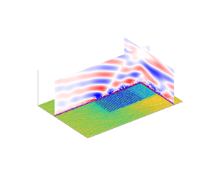Figure 3 illustrates vertical profiles of several quantities of interest averaged over the last $4$ h of the simulations and over the full horizontal directions. Figure 3(a–d) shows the velocity magnitude normalized with the geostrophic wind. The boundary layer extends up to the capping inversion, which limits its growth. All velocity profiles show a common feature, that is, the presence of a super-geostrophic jet near the top of the ABL, which is a typical phenomenon observed in this type of atmospheric conditions. Pedersen et al. (Reference Pedersen, Gryning and Kelly2014) investigated the evolution of this super-geostrophic jet in detail, while, e.g. Goit & Meyers (Reference Goit and Meyers2015, Appendix B) and Allaerts & Meyers (Reference Allaerts and Meyers2015) mathematically derived the existence of such jets by following on the findings of Zilitinkevich (Reference Zilitinkevich1989). We note that this phenomenon is more accentuated for the H150 cases, where a stronger wind shear along with stronger velocity gradients at the top of the ABL are attained. Next, figure 3(e–h) displays the shear stress magnitude, which is non-zero only below the capping inversion, with a quasi-linear profile. We note that varying $\Delta \theta$ and $\varGamma$ results in very minor differences in terms of velocity and shear stresses. Next, figure 3(i–l) shows the flow angle. At turbine hub height, the flow is parallel to the $x$ direction. This is achieved by using the wind-angle controller developed and tuned by Allaerts & Meyers (Reference Allaerts and Meyers2015), which is designed to ensure a desired orientation of the hub-height wind direction ($\varPhi _d =0^\circ$ in this case). Below the turbine-tip height, the flow is almost unidirectional since most of the wind-direction change occurs within the inversion layer, except for deep boundary layers. The geostrophic wind angle, which is the angle between the surface stress and the geostrophic wind velocity, is larger for shallow boundary layers, as noted by Allaerts & Meyers (Reference Allaerts and Meyers2017). Finally, the thermal stratification is illustrated in figure 3(m–p) by means of potential-temperature profiles. For sake of completeness, we also show the neutral cases here. However, we note that those cases are artificially generated (see § 3.3).

Figure 3. Vertical profiles of (a–d) velocity magnitude, (e–h) shear stress magnitude, (i–l) wind direction and (m–p) potential temperature averaged along the full horizontal directions and over the last $4$ h of the simulation. The results are shown for (a,e,i,m) H150, (b,f,j,n) H300, (c,g,k,o) H500 and (d,h,l,p) H1000 cases using various capping-inversion strengths and free-atmosphere lapse rates. Moreover, the profiles are further normalized with $G=10\ {\rm m}\ {\rm s}^{-1}$, $u_{\star,{min}}=0.275\ {\rm m}\ {\rm s}^{-1}$, $|\alpha |_{max}=19.4 ^\circ$ and $\theta _0=288.15$ K. The red dashed line denotes the turbine hub height while the black dashed lines are representative of the rotor dimension. Finally, the grey dashed line represents the averaged inversion-layer height. We note that the results shown here only refer to the precursor simulations.

The various spin-up cases together with some parameters of interest averaged over the last $4$ h of simulation are summarized in table 1. During the spin-up phase, the capping-inversion height moves slightly upward. The increase in inversion-layer height is more accentuated for the shallow boundary-layer cases. For instance, the H150 cases show a growth of $67$ m on average over the 20 h of spin-up. However, the height of the capping inversion is still below turbine-tip height for six of those cases. For the H1000 cases, the boundary-layer height remains unaltered. This result is consistent with the equilibrium theory of Csanady (Reference Csanady1974) and with previous LES findings (Pedersen et al. Reference Pedersen, Gryning and Kelly2014; Allaerts & Meyers Reference Allaerts and Meyers2015, Reference Allaerts and Meyers2017). The capping-inversion strength slightly increases for the majority of the cases while the free-atmosphere stratification remains unchanged. The velocity magnitude at turbine hub height varies between $9.1$ and $9.5\ {\rm m}\ {\rm s}^{-1}$ among all cases, meaning that turbines operate in the region $2$ (Bortolotti et al. Reference Bortolotti, Tarrés, Dykes, Merz, Sethuraman, Verelst and Zahle2019). Moreover, the turbulence intensity at turbine hub height varies from 3.3 % to 4.1 %. These values are in line with those observed by Barthelmie et al. (Reference Barthelmie2009) and Türk & Emeis (Reference Türk and Emeis2010) over the North Sea. The large variance in the Froude number, defined as ${Fr}={U}_B/\sqrt {g'H}$ with $U_B$ the bulk velocity along the $x$ direction (i.e. the streamwise velocity averaged over the full streamwise and spanwise directions and along the boundary-layer height) and $g'=g \Delta \theta /\theta _0$ the reduced gravity, will allow us to analyse the flow response to wind-farm forcing under critical (${Fr} \approx 1$), subcritical (${Fr} \leq 1$) and supercritical (${Fr} \geq 1$) conditions with varying $P_N= {U}_B^2/NGH$ numbers. We note that, while the pressure feedback due to interfacial waves depends upon the ${Fr}$, the $P_N$ number relates to the pressure perturbation induced by internal waves (see Smith (Reference Smith2010) and Allaerts & Meyers (Reference Allaerts and Meyers2019) for more details). Both the ${Fr}$ and $P_N$ number values for all cases are reported in table 1.

3.2. Wind-farm start-up phase

The turbulent fully developed inflow profiles previously discussed are now used to drive the simulation in the main domain, where the turbines impose a drag force on the flow. However, before collecting flow statistics over time, a second spin-up phase is required. In fact, the flow has to adjust to the presence of the farm in the main domain before reaching a new statistically steady state. We name this phase wind-farm start-up. Figure 4 shows the time evolution of the vertical velocity field on an $x$–$z$ plane for case H500-$\Delta \theta$2-$\varGamma$8. The flow divergence induced by the farm drag force displaces upward the capping inversion, which in turn triggers a first train of internal gravity waves in proximity to the first-row turbine location. Vice versa, the flow convergence in the farm wake moves the capping inversion downward, generating a second train of internal waves at the last-row turbine location. This is clearly visible in figure 4(a). The two out-of-phase trains of waves are convected downstream, until they eventually merge at $T=1$ h, as shown in figure 4(e). At this point, the numerical solution is further advanced in time for $1.5$ h. The instantaneous vertical velocity flow field taken at $T=2.5$ h is displayed in figure 4(f). By comparing the numerical solution at $T=1$ h against that obtained at $T=2.5$ h, we note minimal differences. A similar behaviour is observed for the streamwise and spanwise velocity fields (not shown). This means that 1 h of wind-farm spin-up time suffices for the flow to adjust to the farm drag force. We note that other cases have similar velocity magnitude at hub height (see table 1), meaning that the number of flow-through times would be very similar to that of case H500-$\Delta \theta$2-$\varGamma$8. Therefore, similarly to Allaerts & Meyers (Reference Allaerts and Meyers2017) and Lanzilao & Meyers (Reference Lanzilao and Meyers2022), we fix the duration of the wind-farm start-up phase to 1 h, which corresponds to roughly two and a half wind-farm flow-through times. Next, we switch off the wind-angle controller in the precursor simulation and we collect statistics during a time window of $1.5$ h.

Figure 4. Instantaneous contours of vertical velocity for case H500-$\Delta \theta$2-$\varGamma$8 obtained (a–d) during the wind-farm start-up phase, (e) at the end of the wind-farm start-up phase and (f) at the end of the simulation. The $x$–$z$ plane is taken along the centreline of the domain, i.e. at $y=15$ km. The black vertical dashed lines denote the location of the first- and last-row turbine. We note that the fringe region and RDL are not displayed in the plots.

3.3. Construction of a neutral boundary-layer reference case

For each inversion-layer height, we also include a case characterized by the absence of the capping inversion and a neutral free atmosphere, an idea originally proposed by Lanzilao & Meyers (Reference Lanzilao and Meyers2022). To do so, the fringe forcing in the main domain only forces the velocity field to the one provided by the CNBL developed in the precursor domain, leaving the potential temperature constant with height. To give an example, case H500-$\Delta \theta$0-$\varGamma$0 is driven by the flow fields obtained in the precursor simulation of case H500-$\Delta \theta$5-$\varGamma$4, but sets the temperature profile in the main domain to a constant value. Consequently, in this case, the farm operates under the same turbulent inflow velocity profile but in the absence of thermal stratification above the ABL. We note that the same strategy is used for cases H150-$\Delta \theta$0-$\varGamma$0, H300-$\Delta \theta$0-$\varGamma$0 and H1000-$\Delta \theta$0-$\varGamma$0. This is admittedly a numerical construction that does not really exist in reality but allows us to factor out effects due to thermal stratification above the ABL. It has however also some drawbacks. For instance, the capping-inversion height is much lower than the Ekman-layer equilibrium height that the boundary layer would attain in a TNBL. Therefore, in the main domain, the flow within the ABL inevitably starts mixing with the free atmosphere, varying its shear and veer already before reaching the first-row turbine location. In the H150-$\Delta \theta$0-$\varGamma$0 and H300-$\Delta \theta$0-$\varGamma$0 cases, this flow mixing is very high, varying considerably the flow profiles. For instance, the flow angle at the farm entrance measures approximately 10 $^\circ$ in the H150-$\Delta \theta$0-$\varGamma$0 case. However, this effect becomes negligible in the H500-$\Delta \theta$0-$\varGamma$0 and H1000-$\Delta \theta$0-$\varGamma$0 cases, where the flow remains parallel to the streamwise direction and, in general, profiles show very similar results in front of and across the farm, with a farm efficiency of 47.0 % and 46.7 %, respectively. Therefore, we use case H500-$\Delta \theta$0-$\varGamma$0 as a reference simulation for a farm operating in the absence of thermal stratification above the ABL in the rest of this article, and we refer to it as the NBL reference case.

A working example of this idea is given in figure 5(a,b), which displays the flow field obtained in the main domain for the NBL reference case (i.e. H500-$\Delta \theta$0-$\varGamma$0) and the H500-$\Delta \theta$5-$\varGamma$4 case, respectively. The two simulations are driven by the same turbulent inflow profiles. However, the potential-temperature profile is set to a constant in figure 5(a) while figure 5(b) uses the potential temperature provided by the precursor simulations. By comparing the results of these two simulations, it is easy to investigate the effects induced by the thermal stratification above the ABL on the wind-farm flow behaviour. The various differences will be analysed in detail in § 4.

Figure 5. Snapshot of the instantaneous flow field obtained after 2.5 h of simulation time in the (a) NBL reference case and in (b) CNBL conditions. The two simulations correspond to cases H500-$\Delta \theta$0-$\varGamma$0 and H500-$\Delta \theta$5-$\varGamma$4, respectively. The $x$–$y$ plane shows contours of velocity magnitude $(u^2+v^2)^{1/2}$ taken at turbine hub height while the $x$–$z$ and $y$–$z$ planes display the vertical velocity field. The black disks denote the wind-turbine rotor locations. Finally, we note that the fringe region and RDL are not displayed. We remark that the only difference in the NBL reference case consists in the absence of thermal stratification above the ABL.

4.1. Effects of the inversion-layer height on the flow development

We start our analysis with figure 6, which shows the $x$–$z$ plane across the sixth column of turbines of the instantaneous horizontal velocity magnitude together with the base and top of the inversion layer computed by fitting the LES data with the Rampanelli & Zardi (Reference Rampanelli and Zardi2004) model. Every turbine imparts a force on the flow, generating a patch of low wind speed downwind. Figure 6(a) shows that such velocity deficits are very strong in a shallow boundary layer. In fact, the turbine-tip height is in close proximity to the capping-inversion base, which limits energy entrainment and, therefore, flow mixing, slowing down the wake recovery process. Moreover, this also limits the growth of the internal boundary layer (IBL) generated by the wind-turbine wakes expansion. Therefore, to conserve mass, the flow deceleration is mostly compensated by a flow redirection at the sides of the farm, generating high-speed flow channels. This is visible in figure 7(a), which shows the time-averaged turbine-orientation angle with respect to the streamwise direction for all turbines in the farm. Here, the angles between the first- and last-turbine columns vary between $-8^\circ$ and $8^\circ$. The asymmetry with respect to the domain centreline observed in figure 7 is due to the presence of the Coriolis effects. The upward motion caused by the strong flow divergence results in a capping-inversion vertical displacement, which reaches a maximum in proximity to the second-row turbines, with a relative capping-inversion displacement of 42.9 %. A strong wind-speed reduction is also observed in the farm induction region. Furthermore, the low level of energy entrainment also causes a strong wind-farm wake. The interaction between the IBL and capping inversion decreases as $H$ increases. We observe in figure 6(c) that the vertical wake expansion reaches the inversion-layer height only in the farm wake.

Figure 6. Contours of the instantaneous horizontal velocity magnitude in an $x$–$z$ plane taken across the sixth column of turbines, i.e. at $y=15.25$ km, for cases (a) H150-$\Delta \theta$5-$\varGamma$4, (b) H300-$\Delta \theta$5-$\varGamma$4, (c) H500-$\Delta \theta$5-$\varGamma$4, (d) H1000-$\Delta \theta$5-$\varGamma$4 and (e) the NBL reference case. The black lines represent the bottom and top of the inversion layer computed with the Rampanelli & Zardi (Reference Rampanelli and Zardi2004) model. Finally, the location of the turbine rotor disks is indicated with vertical white lines. The NBL reference case refers to simulation H500-$\Delta \theta$0-$\varGamma$0.

Figure 7. Turbine-orientation angle with respect to the streamwise direction for cases (a) H150-$\Delta \theta$5-$\varGamma$4, (b) H300-$\Delta \theta$5-$\varGamma$4, (c) H500-$\Delta \theta$5-$\varGamma$4, (d) H1000-$\Delta \theta$5-$\varGamma$4 and (e) the NBL reference case. The latter refers to simulation H500-$\Delta \theta$0-$\varGamma$0.

For a deep boundary layer, the capping-inversion effects on the wind-farm response become negligible. Here, the IBL does not interact with the inversion layer. This also allows a high-speed flow region to form between the IBL and capping-inversion base, as shown in figure 6(d), which enhances flow mixing and consequently the vertical transport of energy (not shown here), therefore replenishing the turbine and farm wake at a higher rate. This also translates into a much smaller flow redirection at the farm sides since the vertical expansion of the IBL is not constrained by the inversion layer. Figure 7(d) shows variation in turbine-orientation angles only between $-2^\circ$ and $2^\circ$ for this case. In all atmospheres with thermal stratification above the ABL, figure 6 shows that the turbulent structures are damped by the inversion layer, leaving the free atmosphere non-turbulent. A different behaviour is observed in figure 6(e), which illustrates the results obtained in a neutral atmosphere. The turbulence structures at the top of the boundary layer are not damped by buoyant forces in this case, allowing the IBL to reach higher altitudes. Here, the reduction in wind speed caused by the turbines is solely balanced by the boundary-layer thickening. In fact, figure 7(e) shows that all turbines have positive orientation angles, which gradually increase towards the last row.

The upward displacement of the inversion layer, which has to be considered as an interfacial wave, brings air with a lower potential temperature to a higher altitude, generating a cold anomaly. This is illustrated in figure 8, which shows the $x$–$z$ plane of the time-averaged potential-temperature perturbation field together with the base and top of the inversion layer, averaged in the horizontal directions along the farm width. The negative perturbation in the potential-temperature field is about 7 and 2 K in cases H150-$\Delta \theta$5-$\varGamma$4 and H1000-$\Delta \theta$5-$\varGamma$4, respectively. This considerable difference is caused by the higher inversion-layer displacement attained in case H150-$\Delta \theta$5-$\varGamma$4 (and in shallow boundary-layer flows, in general), which measures 42.9 % (i.e. 90 m) against the 3.8 % (i.e. 40 m) obtained for case H1000-$\Delta \theta$5-$\varGamma$4. We note that the cold anomaly extends to the farm induction region in all cases. Moreover, the interfacial waves along the capping inversion are also clearly visible. In fact, figure 8 shows that the interfacial-wave crests correspond to high potential-temperature perturbations. Finally, the flow acceleration in the wind-farm wake pushes the inversion layer downward, generating a hot anomaly. Since the ABL itself is neutral, potential-temperature perturbations do not occur below the inversion layer.

Figure 8. Contours of the time-averaged potential-temperature perturbation with respect to the inflow in an $x$–$z$ plane further averaged in the $y$ direction along the width of the farm for cases (a) H150-$\Delta \theta$5-$\varGamma$4, (b) H300-$\Delta \theta$5-$\varGamma$4, (c) H500-$\Delta \theta$5-$\varGamma$4 and (d) H1000-$\Delta \theta$5-$\varGamma$4. The black lines represent the bottom and top of the inversion layer computed with the Rampanelli & Zardi (Reference Rampanelli and Zardi2004) model. Finally, the location of the turbine rotor disks is indicated with vertical black lines.

As noted by Smith (Reference Smith2010) and Allaerts & Meyers (Reference Allaerts and Meyers2017), variations in the potential-temperature field are strongly correlated to pressure perturbations. In fact, a cold anomaly translates into a higher column of cold and heavy air, which locally increases pressure. Vice versa, a hot anomaly generates a region of low pressure. This behaviour is illustrated in figure 9, which shows an $x$–$z$ plane of the time-averaged pressure-perturbation field together with the base and top of the inversion layer, averaged in the horizontal directions along the farm width. The strong cold anomaly generated in shallow boundary layers gives rise to strong increases in pressure, with a peak in the farm entrance region. This strong counteracting pressure gradient extends across the whole farm induction region. By comparing figure 9(a,d), it becomes clear that the unfavourable pressure gradient is inversely proportional to the capping-inversion height. The low pressure region downwind of the farm generated by the hot anomaly gives rise to a favourable pressure gradient across the farm that enhances the wake recovery mechanism. Finally, figure 9(e) shows the pressure perturbation obtained in a neutrally stratified atmosphere. Here, the unfavourable pressure gradient, which is solely due to the flow slow down caused by the cumulative turbine induction, is an order of magnitude lower than that obtained in stratified atmospheres and only extends up to roughly six rotor diameters upstream of the first-row turbines. Moreover, also the favourable pressure gradient is negligible when compared with that obtained in the presence of thermal stratification above the ABL.

Figure 9. Contours of the time-averaged pressure perturbation with respect to the inflow in an $x$–$z$ plane further averaged in the $y$ direction along the width of the farm for cases (a) H150-$\Delta \theta$5-$\varGamma$4, (b) H300-$\Delta \theta$5-$\varGamma$4, (c) H500-$\Delta \theta$5-$\varGamma$4, (d) H1000-$\Delta \theta$5-$\varGamma$4 and (e) the NBL reference case. The black lines represent the bottom and top of the inversion layer computed with the Rampanelli & Zardi (Reference Rampanelli and Zardi2004) model. Finally, the location of the turbine rotor disks is indicated with vertical black lines. The NBL reference case refers to simulation H500-$\Delta \theta$0-$\varGamma$0.

4.2. Effects of the inversion-layer strength and free-atmosphere lapse rate on the flow development

Following the work of Klemp & Lilly (Reference Klemp and Lilly1975) and Vosper (Reference Vosper2004), Sachsperger, Serafin & Grubišić (Reference Sachsperger, Serafin and Grubišić2015) derived a two-dimensional gravity-wave linear model in which they found that the wavenumber $k_x$ of the interfacial waves depends upon the capping-inversion strength and Brunt–Väisälä frequency as follows:

(4.1)\begin{equation} k_x = \frac{g \Delta \theta}{2{U}_B^2\theta_0} + \frac{N^2 \theta_0}{2 g \Delta \theta}. \end{equation}

Sachsperger et al. (Reference Sachsperger, Serafin and Grubišić2015) showed that, under a constant Brunt–Väisälä frequency, the interfacial-wave horizontal wavelength $\lambda _x = 2 {\rm \pi}/ k_x$ is inversely related to the strength of the capping inversion $\Delta \theta$. Consequently, when $\varGamma$ is kept constant, a stronger capping inversion supports interfacial waves with a lower wavelength. This is visible in figure 10, where we compare $x$–$y$ planes taken at the turbine hub height of velocity magnitude, vertical velocity and pressure perturbation of three simulations where the only varying parameter is $\Delta \theta$. Figure 10(a–c) shows that a higher $\Delta \theta$ causes a higher flow speed up at the farm sides. This is due to the fact that, on average, a high inversion-layer strength reduces the capping-inversion upward displacement. Consequently, the flow rate at the farm sides has to increase to compensate for the limited thickening of the boundary layer. The vertical velocity fields shown in figure 10(e–g) clearly illustrate that the upward motion caused by these waves propagates down to turbine hub height, generating patches of low and high wind speed. According to (4.1), the interfacial-wave wavelength is 6.1 and 4 km for cases H500-$\Delta \theta$5-$\varGamma$1 and H500-$\Delta \theta$8-$\varGamma$1, which is in line with the 7.3 km and 4.9 km observed in figure 10(f,g). However, $\lambda _x$ measures 10.1 km for case H500-$\Delta \theta$2-$\varGamma$1, which corresponds to 2/3 of the farm length. For this case, interfacial waves are not visible in figure 10(a,e,i). We speculate that a longer domain is necessary for these waves to become clearly visible. We also remark the presence of a V-shape pattern at the farm sides, which is very similar to that noted by Allaerts & Meyers (Reference Allaerts and Meyers2019). This phenomenon will be further discussed in § 4.3.

Figure 10. Contours of the time-averaged (a–d) velocity magnitude, (e–h) vertical velocity and (i–l) pressure perturbation in an $x$–$y$ plane taken at turbine hub height for cases (a,e,i) H500-$\Delta \theta$2-$\varGamma$1, (b,f,j) H500-$\Delta \theta$5-$\varGamma$1, (c,g,k) H500-$\Delta \theta$8-$\varGamma$1 and (d,h,l) the NBL reference case. The location of the turbine rotor disks is indicated with vertical white lines. The NBL reference case refers to simulation H500-$\Delta \theta$0-$\varGamma$0.

Finally, figure 10(i–k) displays pressure perturbation with respect to the inflow value. Here, we note that the pressure oscillations seem to be superimposed on top of a large-scale gradient. We believe that the large-scale gradient is caused by the global displacement of the capping inversion. Interfacial waves further corrugate this surface, giving rise to the pressure oscillations particularly visible in figure 10(j,k), which have a similar wavelength to the trapped lee waves observed in figure 10(f,g). Furthermore, we note that the footprint of the counteracting pressure gradient in the farm induction region together with the favourable one across the farm is positively correlated with $\Delta \theta$. However, case H500-$\Delta \theta$5-$\varGamma$4 shows the highest pressure-perturbation magnitude, the latter being roughly 1.5 times that obtained in case H500-$\Delta \theta$2-$\varGamma$1. We speculate that this is due to the chocking effect (Smith Reference Smith2010), since ${Fr}=0.99$ in this case. Moreover, the V-shape pattern causes a favourable pressure gradient also at the farm sides, which further enhances the channelling effects. We note that the recycling of pressure perturbations along the spanwise direction suggests that the domain width should be further increased in future studies. Finally, figure 10(d,h,l) shows the results obtained in the NBL reference case. As mentioned earlier, the pressure perturbations are at least one order of magnitude lower than in cases with thermal stratification above the ABL. This explains the absence of velocity reductions several kilometres upstream of the farm together with a monotonic decrease in velocity magnitude between the first- and last-row turbines.

We now turn our attention to the effects of changes in the free-atmosphere lapse rate. Equation (4.1) shows that the interfacial-wave horizontal wavelength is negatively correlated with the Brunt–Väisälä frequency. This means that an increases in free-atmosphere stability results in a lower $\lambda _x$ value. Figure 11 clearly illustrates this behaviour. As $\varGamma$ increases, air parcels find more resistance in displacements along the vertical direction due to the stronger buoyant forces. Therefore, a stronger free-lapse rate damps waves along the inversion layer, limiting its vertical displacement. Consequently, a lower cold anomaly is generated, which leads to lower pressure perturbations. This is visible when comparing figure 11(i,k), which shows $x$–$y$ planes of pressure perturbations at turbine hub height obtained with $\varGamma =1\ {\rm K}\ {\rm km}^{-1}$ and $\varGamma =8\ {\rm K}\ {\rm km}^{-1}$, respectively, while keeping all other parameters constant. This also implies that the hydrostatic flow-blockage effect reduces as the stability of the free atmosphere increases in the presence of a strong capping-inversion strength, as shown in figure 11(a–c). This result is in contrast with findings of Abkar & Porté-Agel (Reference Abkar and Porté-Agel2013) and Wu & Porté-Agel (Reference Wu and Porté-Agel2017), who observed that changing the free-lapse rate from $1\ {\rm K}\ {\rm km}^{-1}$ to $10\ {\rm K}\ {\rm km}^{-1}$ caused a power drop of about 35 %. However, in their study, they were at the same time varying the capping-inversion height and strength, which explains this difference in power output. Finally, figure 11(e–g) shows the vertical velocity fields, where the V-shape pattern at the farm sides together with interfacial-wave effects are clearly visible. Interestingly, we also observe slanted lines at the left side of the farm with an angle of $29^\circ$ with respect to the streamwise direction. We note that this effect is related to the perturbation introduced by the single turbines and will be further discussed in § 4.3. For the sake of comparison, we report again the results obtained for the NBL reference case in figure 11(d,h,l).

Figure 11. Contours of the time-averaged (a–d) velocity magnitude, (e–h) vertical velocity and (i–l) pressure perturbation in an $x$–$y$ plane taken at turbine hub height for cases (a,e,i) H300-$\Delta \theta$8-$\varGamma$1, (b,f,j) H300-$\Delta \theta$8-$\varGamma$4, (c,g,k) H300-$\Delta \theta$8-$\varGamma$8 and (d,h,l) the NBL reference case. The location of the turbine rotor disks is indicated with vertical white lines. The NBL reference case refers to simulation H500-$\Delta \theta$0-$\varGamma$0.

4.3. Comparison between LES results and gravity-wave linear-theory models

The simplicity of gravity-wave linear-theory models contributed to their spread in analysing mountain-wave phenomena. A wide variety of this type of model can be found in Gill (Reference Gill1982), Nappo (Reference Nappo2002), Lin (Reference Lin2007), Sutherland (Reference Sutherland2010) and Teixeira (Reference Teixeira2014). More recently, the same theory has been applied to wind-farm studies, since the latter can be considered as a ‘permeable mountain’. Examples of these models can be found in Smith (Reference Smith2010), Allaerts & Meyers (Reference Allaerts and Meyers2018), Allaerts & Meyers (Reference Allaerts and Meyers2019), Devesse et al. (Reference Devesse, Lanzilao, Jamaer, van Lipzig and Meyers2022) and Smith (Reference Smith2022, Reference Smith2023). In the current section, we perform a comparison of our results against some of the simplest wind-farm gravity-wave linear-theory models.

Figure 12 compares the internal gravity-wave pattern obtained in three LES against the results obtained with a simple two-dimensional gravity-wave linear-theory model (Nappo Reference Nappo2002). The latter is a quasi-analytical model that takes as an input the shape of the obstacle, assumed impermeable. The obstacle shape also provides the bottom boundary conditions to the system of equations. In the current study, the inversion-layer displacement shown in figure 15(a–d) defines the obstacle shape. For the sake of clearness, we briefly explain this linear model in Appendix C. We remark the excellent agreement between our results and linear theory, particularly in terms of gravity-wave phase line and vertical wavelength. Moreover, the slanted region tilted downstream of zero vertical velocity that forms near the trailing edge of the farm is captured by both models. This supports the idea that this phenomenon is not a manifestation of internal gravity-wave reflection but is rather due to the interaction between two out-of-phase trains of internal waves triggered by the first- and last-row turbines; see figure 4. We believe that this good comparison is mostly a result of the effort spent in properly developing and calibrating the buffer regions in the main domain. We note that a discussion on the internal gravity-wave reflectivity is reported in Appendix D.

Figure 12. Contours of the time-averaged vertical velocity field in an $x$–$z$ plane further averaged along the farm width for cases (a) H300-$\Delta \theta$5-$\varGamma$1, (b) H300-$\Delta \theta$5-$\varGamma$4 and (c) H300-$\Delta \theta$5-$\varGamma$8. (d–f) Vertical velocity field obtained with the two-dimensional gravity-wave linear-theory model described in Appendix C. For instance, the internal waves in panel (d) are excited by an obstacle with shape given by the capping-inversion vertical displacement obtained in case H300-$\Delta \theta$5-$\varGamma$1. The vertical black dashed lines in panel (a–c) denote the location of the first- and last-row turbines while the location of the turbine rotor disks in panels (a–c) are indicated with vertical white lines.

Next, figure 13 displays a $x$–$y$ plane of the time-averaged vertical velocity field taken at turbine-tip height for case H300-$\Delta \theta$5-$\varGamma$1. The flow deceleration causes a strong upward motion in the proximity of the first rows of turbines, which results in interfacial waves along the capping inversion. The upward and downward motion that these waves generate is very visible in figure 13, both in and around the farm.

Figure 13. Contours of the time-averaged vertical velocity field in an $x$–$y$ plane taken at turbine-tip height for case H300-$\Delta \theta$5-$\varGamma$1. The definition of the farm V-shape angle $\beta _{les}$ together with the angle that the slanted lines make with the horizontal $\gamma _{les}$ are reported in the figure. The location of the turbine rotor disks is indicated with vertical white lines.

Two additional distinct phenomena take place. First, we observe a V-shape pattern around the farm that has already been observed and investigated by Allaerts & Meyers (Reference Allaerts and Meyers2019). They reported that the angle of the pair of characteristic lines that gives rise to this pattern is only dependent on the Froude number and is given by

(4.2)\begin{equation} \beta_{lin} = \arctan{\left(\left( {Fr}^2-1\right)^{-1/2}\right)}, \end{equation}

where the Froude number is defined as a ratio between a boundary-layer velocity scale (i.e. ${U}_B$) and the interfacial-wave phase speed. In shallow-water wave theory, the phase speed is given by $\sqrt {g'H}$ (Acheson Reference Acheson1990; Sutherland Reference Sutherland2010). This theory holds under the assumption that $L>4{\rm \pi} H$, where $L$ denotes the length scale of the forcing. If we use the distance between first- and last-row turbines as a length scale (i.e. $L=L_x^f$), this relation holds and the Froude number is therefore defined as ${Fr}={U}_B/\sqrt {g'H}$ (Smith Reference Smith2010; Allaerts & Meyers Reference Allaerts and Meyers2019). For instance, the Froude number is 1.29 for the case shown in figure 13, which results in $\beta _{lin}=50.8^\circ$. This value is in excellent agreement with that observed in the LES results, which measures $\beta _{les}=51^\circ$. Equation (4.2) shows that the angle is well defined only for supercritical flows. In subcritical cases the characteristic lines become imaginary and no V-shape pattern occurs around the farm (Allaerts & Meyers Reference Allaerts and Meyers2019). The second pattern observed in figure 13 is a set of slanted lines, and is related to the perturbation introduced by the turbine spacing. In fact, if we use as a length scale the equivalent turbine spacing $S_e = D \sqrt {s_x s_y}$, then we should define the interfacial-wave phase speed using deep-water wave theory, which holds when $L< H/{\rm \pi}$. We note that the streamwise or spanwise spacings could also be a candidate for the length-scale definition. However, we cannot make such distinction as $S_e = S_x = S_y$ in our work. Using this theory, the Froude number is defined as

(4.3)\begin{equation} {Fr}_{dw} = \frac{{U}_B}{\sqrt{\dfrac{g'S_e}{2 {\rm \pi}} \mathrm{tanh}\left( \dfrac{2 {\rm \pi}H}{S_e}\right)}}, \end{equation}

where the denominator represents the interfacial-wave phase speed. This Froude number measures 1.88 for case H300-$\Delta \theta$5-$\varGamma$1. Using (4.2), this results in an angle of $32.1^\circ$, which we denote with $\gamma _{lin}$. Also, this angle is in good agreement with that observed in the LES results, which measures $\gamma _{les}=28^\circ$. We note that the lines that make the angles $\beta _{les}$ and $\gamma _{les}$ with the horizontal are also reported in figure 13. While the angle is explained by (4.2), we also see in figure 13 that these slanted lines only propagate along the left side of the farm. We speculate that this is due to the asymmetry generated by the Coriolis force.

The angles $\beta _{les}$ and $\gamma _{les}$ are measured by carefully aligning a slanted line to the pattern observed in the vertical velocity field, as shown in figure 13. A comparison between the $\beta _{lin}$ and $\beta _{les}$ angles for supercritical flows is shown in figure 14(a). Overall, we observe an excellent agreement, with values collapsing along the diagonal and a coefficient of determination of 0.86. Next, figure 14(b) compares the angle formed by the slanted lines triggered by the turbine spacing. We see again a good agreement, with $\gamma _{les}$ slightly lower than $\gamma _{lin}$ in deeper boundary layers. Finally, figure 14(c) shows a comparison between the interfacial-wave horizontal wavelength obtained in LES against that evaluated with linear theory, i.e. using (4.1). For this case, the coefficient of determination measures 0.89, indicating a very strong correlation and, therefore, good agreement between linear theory and LES results.

Figure 14. (a,b) Comparison of the $\beta$ and $\gamma$ angles measured in the LES results against the values predicted by linear theory (Allaerts & Meyers Reference Allaerts and Meyers2019). (c) Comparison of trapped-wave horizontal wavelength between LES results and the linear-theory model of Vosper (Reference Vosper2004) and Sachsperger et al. (Reference Sachsperger, Serafin and Grubišić2015) (i.e. (4.1)). (d) Comparison of maximum inversion-layer vertical displacement between the LES results and the one-dimensional linear model developed by Allaerts & Meyers (Reference Allaerts and Meyers2018). The $R^2$ value denotes the coefficient of determination.

Allaerts & Meyers (Reference Allaerts and Meyers2018) derived a linear one-dimensional model for the capping-inversion vertical displacement in response to a drag force imposed within the whole ABL. The governing equation reads as

(4.4)\begin{equation} \left(1 - \frac{1}{{Fr}^2} \right) \frac{\partial \eta}{\partial x} = c_t {\varPi}(x) -2 \left( c_t \varPi(x) + c_d \right) \frac{\eta}{H} - \frac{1}{P_N} \mathcal{G}_N(\eta), \end{equation}

where $\varPi (x)$ denotes a step function with support going from the start to the end of the farm and $c_d=u_\star /U_B$ represents the friction with the ground. Moreover, the thrust force imposed on the flow scales linearly with $c_t$, which is defined as

(4.5)\begin{equation} c_t=\frac{1}{2}\frac{{\rm \pi} C_T}{4s_x s_y}\eta_w \gamma_v \end{equation}

with $\gamma _v = U_{B,r}^2/U_B^2$ a wind-profile shape factor, where $U_{B,r}^2$ denotes the velocity in the streamwise direction obtained in the precursor simulation averaged over the full streamwise and spanwise directions and along the turbine rotor height. Moreover, $\eta _w$ denotes the wake efficiency, which is later defined in (4.7a,b). Finally, $\mathcal {G}_N(\eta )$ is a linear operator that accounts for internal-wave effects and is expressed as

(4.6)\begin{equation} \mathcal{G}_N(\eta) = \frac{1}{2 {\rm \pi}} \int |k| \left( \int \eta(x') {\rm e}^{-{\rm i}kx'}\,{{\rm d}\kern0.7pt x}'\right) {\rm e}^{{\rm i}kx} \,{\rm d}k. \end{equation}

We refer to Appendix 2 in Allaerts & Meyers (Reference Allaerts and Meyers2018) for a full derivation of (4.4). Given the atmospheric state, (4.4) predicts the capping-inversion displacement along the streamwise direction. Furthermore, we name the maximum inversion-layer vertical displacement obtained with (4.4) and with the LES results as $\mathrm {max}(\eta _{lin})$ and $\mathrm {max}(\eta _{les})$, respectively. These two quantities are displayed in figure 14(d), which shows a good match except for cases H150, for which $\mathrm {max}(\eta _{lin}) < \mathrm {max}(\eta _{les})$. The coefficient of determination is zero in this case, as this metric is very sensitive to outliers. We note that the values of $\eta _w$, $\beta _{les}$, $\gamma _{les}$, $\lambda _{x,{les}}$ and $\mathrm {max}(\eta _{les})$ for all cases are summarized in table 2.

Table 2. Overview of the simulation results including the farm V-shape angle $\beta _{les}$, the slanted lines angle $\gamma _{les}$, the trapped-wave horizontal wavelength $\lambda _{x,{les}}$, the maximum inversion-layer vertical displacement $\mathrm {max}(\eta _{les})$, the reflectivity $r$, the non-local efficiency $\eta _{nl}$, the wake efficiency $\eta _w$, the farm efficiency $\eta _f$, the first-row turbine power output and the power output of a turbine operating in isolation normalized with a reference air density $P_1/\rho _0$ and $P_\infty /\rho _0$, respectively, and the unfavourable and favourable pressure gradients magnitude $\Delta p_u$ and $\Delta p_f$, respectively. We remark that the NBL reference case refers to simulation $\textrm{H}500-\Delta \theta 0-\varGamma 0$.

In this section we have seen that our results match well when compared against various gravity-wave linear-theory models found in the literature. This further confirms that the LES results are not distorted by the domain boundaries and provide an interesting benchmark for the development, validation and calibration of existing and future low- and medium-fidelity wind-farm models.

4.4. Comparison of flow profiles

We now investigate and compare flow profiles among all cases. Results are reported in figure 15, which displays time-averaged flow profiles as a function of the streamwise direction. We start the analysis with figure 15(a–d) that displays the streamwise variation of vertical inversion-layer displacement, here denoted with $\eta$, further averaged along the farm width. For the CNBL cases, $\eta$ is defined as the difference between the capping-inversion top evaluated in precursor and main domains using the Rampanelli & Zardi (Reference Rampanelli and Zardi2004) model. It is interesting to see that in the presence of thermal stratification above the ABL, the flow reacts to the presence of the farm several kilometres upstream. Cases with a weak inversion layer show higher displacements, independently from the inversion-layer height. This is due to the weak resistance to vertical motion that air parcels have in such cases. As $\Delta \theta$ increases, interfacial waves with a lower wavelength get excited within the farm and in its wake. As noted previously, a stronger free atmosphere limits the displacement of the inversion layer, particularly within the first couple of turbine rows. Overall, shallow boundary layers tend to show higher inversion-layer vertical displacements than deeper ones. Moreover, $\eta$ sharply decreases downwind of the last row of turbines in all cases, as a response to the flow acceleration in the wind-farm wake. In the NBL reference case, the absence of thermal stratification above the ABL allows for higher growth of the boundary layer. In this case, $\eta$, which is computed as a streamline, shows a monotonic growth across the farm, with a maximum displacement obtained at the last-row turbine location.

Figure 15. Time-averaged (a–d) capping-inversion displacement, (e–h) potential-temperature perturbation, (i–l) pressure perturbation and (m–p) horizontal velocity magnitude averaged over the farm width as a function of the streamwise direction. The potential-temperature perturbation is further averaged over the capping-inversion thickness, while the other quantities are averaged over the turbine rotor height. Moreover, the cases are organized per capping-inversion height. The vertical dashed black lines denote the location of the first- and last-row turbines.

Perturbations in the potential-temperature field are shown in figure 15(e–f), averaged within the capping-inversion height and along the farm width. As $H$ increases, the cold anomaly reduces in magnitude. For instance, the minimum negative temperature perturbation is $-1.4$ K for the H1000 cases, while it attains a value of $-4.6$ K in the H150 cases. Even when the inversion-layer displacement is limited by high $\Delta \theta$ values, the strong inversion that characterizes such cases generates higher temperature differences, which translate into stronger pressure perturbations. The latter are shown in figure 15(i–l), averaged along the farm width and within the turbine rotor height. Here, we observe that the cases with strong unfavourable and favourable pressure gradients are those with a strong inversion layer. For instance, the counteracting pressure gradient in case H300-$\Delta \theta$8-$\varGamma$1 is 4.4 times that obtained in case H300-$\Delta \theta$2-$\varGamma$1. Pressure feedbacks in the neutral reference case are negligible when compared with those obtained in the CNBL cases. For instance, case H300-$\Delta \theta$5-$\varGamma$4, which figure 2 defines as a highly probable atmospheric state over the North Sea, has a 14 times stronger unfavourable pressure gradient than the NBL reference case. However, we should note that all stratified cases are also characterized by a favourable pressure gradient through the farm, while the NBL reference case does not show this feature.

The pressure-perturbation effects on the velocity magnitude are evident in figure 15(m–p). The NBL reference case shows a reduction in wind speed only several rotor diameters upstream of the farm. Consequently, the velocity at the first-row turbine location is always higher than in the cases with thermal stratification above the ABL. Interestingly, the vertical motion generated by the interfacial waves at the capping-inversion height has direct consequences in terms of velocity magnitude at the turbine hub height, where significant oscillation in velocity magnitude within the farm and in its wake are observed for cases with a strong capping inversion. For instance, the velocity magnitude at the fourth-row turbine location is 5 % higher than that measured at the farm leading edge for case H300-$\Delta \theta$8-$\varGamma$1. As $H$ increases, the flow response becomes less sensitive to changes in $\Delta \theta$ and $\varGamma$. In fact, as the inversion-layer height approaches the equilibrium height of the TNBL, its effects on the farm–ABL interactions become smaller. Consequently, the velocity profiles and pressure perturbation of the CNBL cases get closer to those of the NBL reference case, as shown in figure 15(l,p). We remark that a stronger blockage effect and velocity deficits in shallow boundary layers have been observed also in SCADA data from the Nordsee Ost and Amrumbank West wind farms located in the German Bight area (Cañadillas et al. Reference Cañadillas, Foreman, Steinfeld and Robinson2023) and in a previous study (Allaerts & Meyers Reference Allaerts and Meyers2017).

Cases H500-$\Delta \theta$8-$\varGamma$4, H1000-$\Delta \theta$8-$\varGamma$1 and H1000-$\Delta \theta$8-$\varGamma$4 in particular show oscillations in the capping-inversion displacement and temperature perturbation already in the farm induction region. Most likely, these are spurious effects introduced by the fringe region. In fact, Lanzilao & Meyers (Reference Lanzilao and Meyers2023b) have shown that their wave-free fringe-region technique can still introduce some perturbations in the domain of interest for a combination of low Fr and $P_N$ numbers, which characterize these three cases; see table 1.

Finally, figure 16 focuses on the pressure build-up measured at the first-row turbine location along the spanwise direction. Here, the inverse relationship between capping-inversion height and counteracting pressure gradient is evident. Moreover, a deep boundary layer makes the simulation quasi-independent of changes in $\Delta \theta$ and $\varGamma$, as all profiles collapse in figure 16(d). However, the pressure build-up in all CNBL cases still remains higher than that attained in the NBL reference case. Figure 16 also shows that turbines situated in the centre of the farm experience a higher counteracting pressure gradient than those located at the farm sides. The asymmetry of the profiles with respect to the domain centreline is caused by the presence of the Ekman layer.

Figure 16. Pressure perturbation as a function of the domain width taken at $x=18$ km (i.e. the location of the first-row turbines) and further averaged over the turbine rotor height for cases (a) H150, (b) H300, (c) H500 and (d) H1000. The vertical dashed black lines denote the location of the first- and last-column turbines.

4.5. Wind-farm power production

The time- and row-averaged turbine power output normalized with the first-row turbine power is displayed in figure 17 organized per capping-inversion strength, showing that cases with equal $\Delta \theta$ have similar trends. Figure 17(a) shows that cases with weak capping-inversion height have similar power output per turbine row. The farm has a staggered layout, therefore, the high-speed channels that form between the turbines in the first row allow for a slightly higher power generation at the second row (McTavish et al. Reference McTavish, Rodrigue, Feszty and Nitzsche2015; Meyer Forsting, Troldborg & Gaunaa Reference Meyer Forsting, Troldborg and Gaunaa2017). After a drop of about 50 % between the second and third row, the power remains approximately constant, with a minor increase towards the farm trailing edge for the cases with thermal stratification above the ABL. As the inversion-layer strength increases, power fluctuations are observed within the farm. These are mostly caused by the vertical motion generated by interfacial waves. Consequently, the power does not show a monotonic trend across the farm. Instead, the fifth row often extracts more power than the third row when $\Delta \theta =5$ K, with differences up to 40 %. A more extreme behaviour is observed in figure 17(c), where in three cases a waked row extracts more power than the first row. Moreover, the strong favourable pressure gradient that develops across the farm in cases with a strong inversion layer also leads to an increase in power production towards the end of the farm. This phenomenon is accentuated in shallow boundary layers. For instance, the difference in power output between first- and last-row turbines is only about 8 % in case H300-$\Delta \theta$8-$\varGamma$4, while the last-row turbines produce 23 % more power than the first row in case H150-$\Delta \theta$8-$\varGamma$1.

Figure 17. Averaged power output per turbine row normalized by (a–c) $P_1$ of the respective simulation and (d–f) $P_\infty$ of the respective inversion-layer height obtained with a capping-inversion strength of (a,d) $\Delta \theta =2$ K, (b,e) $\Delta \theta =5$ K and (c,f) $\Delta \theta =8$ K under different inversion-layer heights and free-atmosphere lapse rates. Here, $P_1$ denotes the averaged power outputs of first-row turbines while $P_\infty$ represents the power output of a turbine operating in isolation obtained with the single-turbine simulations – see Appendix B.

Figure 17(d–e) shows the same results but normalized with $P_\infty$, that is, the power output of a turbine operating in isolation. In the CNBL cases, the ratio $P_1/P_\infty$ (i.e. the non-local efficiency) is always much lower than 1, with a minimum of 0.26 attained in case H150-$\Delta \theta$8-$\varGamma$1. Moreover, the flow-blockage effect is much more sensitive to the inversion-layer height in the presence of strong capping inversion, as shown in figure 17(f). In the neutral reference case, $P_1/P_\infty \approx 1$. Once more, this suggests that the flow deceleration in the farm induction region is mostly related to atmospheric gravity waves. Moreover, the power output keeps decreasing towards the farm trailing edge in the NBL reference case, while a power increase is observed for the majority of the CNBL cases. This is due to the favourable pressure gradient acting as an energy source across the farm. We note that the value of $P_1$ and $P_\infty$ for all cases are summarized in table 2.

4.6. Wind-farm efficiencies

We now turn our attention to the wind-farm efficiency. Similarly to Allaerts & Meyers (Reference Allaerts and Meyers2018), we define the farm efficiency as $\eta _f = \eta _w \eta _{nl}$, with

(4.7a,b)\begin{equation} \eta_w = \frac{P_{tot}}{N_t P_1}, \quad \eta_{nl}=\frac{P_1}{P_\infty} \end{equation}

where $\eta _w$ and $\eta _{nl}$ denote the wake and non-local efficiency, respectively. Moreover, $N_t$ indicates the number of turbines, $P_{tot}$ the total farm power, $P_1$ the averaged power output of first-row turbines while $P_\infty$ represents the power output of a turbine operating in isolation. The latter is evaluated using the single-turbine simulations discussed in Appendix B.

The various efficiencies are illustrated in figure 18 for all cases, with values also reported in table 2. Figure 18(a) shows that the strong counteracting pressure gradient that characterizes shallow boundary layers causes $\eta _{nl}$ to be lower in the H150 cases than in the H1000 cases. The highest non-local efficiency is attained in the NBL reference case, showing that the cumulative turbine induction has a minor contribution to the flow-blockage effect for this case. The wake efficiency is shown in figure 18(b). As hypothesized by Allaerts & Meyers (Reference Allaerts and Meyers2018), a low non-local efficiency leads to a higher wake efficiency. In fact, the accumulation of potential energy caused by the flow slow down in front of the farm is converted back into kinetic energy that accelerates the flow across the farm (Allaerts & Meyers Reference Allaerts and Meyers2018). This negative correlation is clearly visible when comparing results in figure 18(a,b). We note that case H150-$\Delta \theta$8-$\varGamma$1 has a wake efficiency greater than 1. For this atmospheric condition, the average power generated by the waked rows is higher than that extracted by first-row turbines. The absence of favourable pressure gradients across the farm causes the wake efficiency of the NBL reference case to be among the lowest. Finally, figure 18(c) displays the overall farm efficiency. The farm efficiency in the H150 and H300 cases is lower than the NBL reference case. For the H500 and H1000 cases, the farm efficiency becomes higher than the NBL reference value. This further highlights the strong influence that the capping-inversion height has on the wind-farm power output. Moreover, we observe that the farm efficiency is positively related with $\varGamma$ in the majority of the cases. We note that the error bars representing the 95 % confidence interval computed with the moving block bootstrapping method for all efficiencies are in the order of $\pm 1\,\%$ and for this reason are not shown in figure 18.

Figure 18. (a) Non-local, (b) wake and (c) farm efficiency as a function of all simulation cases. The cases with thermal stratification above the ABL are represented by a circle while the NBL reference case is marked with a square. The horizontal grey dashed line indicates the relative efficiency value obtained in the NBL reference case.

Next, we investigate how the non-local and wake efficiencies scale with the atmospheric state. In a first attempt, we plot the efficiencies against the ${Fr}$ and $P_N$ numbers, which are the two non-dimensional groups that govern gravity-wave effects. Results are shown in figure 19. The lowest values of non-local efficiency are attained for ${Fr} \approx 1.3$. Figure 19(b) shows that, in general, the non-local efficiency decreases as $P_N$ increases. The wake efficiency shown in figure 19(c,d) shows an opposite trend, as expected. Overall, values remain scattered along the parameter space and strong trends are not observed.

Figure 19. (a,b) Non-local and (c,d) wake efficiency as a function of the (a,c) Fr and (b,d) $P_N$ numbers.

In the previous sections we have seen that gravity-wave induced pressure gradients play a primary role in the flow dynamics. Therefore, in a second attempt, we try to scale the farm efficiencies against these pressure feedbacks. In particular, we define $\Delta p_u = ( \langle \,\bar{p} \rangle _{f,r}(x_{ft}) - \langle \,\bar{p} \rangle _{f,r}(x_{in}) )/\rho _0$ and $\Delta p_f = ( \langle \,\bar{p} \rangle _{f,r}(x_{lt}) - \langle \,\bar{p} \rangle _{f,r}(x_{ft}) )/\rho _0$, where $x_{in}=0$ km represents the main domain inflow. Moreover, $x_{ft}=18$ km and $x_{lt}=32.85$ km denote the location of the first- and last-row turbines, respectively. Given this definition, $\Delta p_u$ and $\Delta p_f$ quantify the pressure feedback upstream and across the farm, respectively. Figure 20(a) shows the non-local efficiency as a function of $\Delta p_u$ normalized by the geostrophic wind. Here, we can observe a very strong negative correlation, with coefficient of determination close to unity. This is expected since the non-local efficiency quantifies the flow slow down in front of the farm, which depends on the magnitude of the unfavourable pressure gradient. An opposite trend is visible in figure 20(d), where the wake efficiency shows a strong positive correlation with $\Delta p_f$, confirming the role of the favourable pressure gradient in accelerating the wake recovery mechanism. High coefficients of determination are also observed in figure 20(b,c), as a consequence of the natural correlation between unfavourable and favourable pressure gradients. The latter is shown in figure 21. Both the favourable and unfavourable pressure gradient magnitude decrease as the capping-inversion height increases, with the lowest value attained in the NBL reference case (see also table 2). Moreover, $\Delta p_f$ is higher than $\Delta p_u$ in the majority of the cases.

Figure 20. (a,b) Non-local and (c,d) wake efficiency as a function of the (a,c) unfavourable and (b,d) favourable pressure gradients magnitude normalized by the geostrophic wind. The $R^2$ value denotes the coefficient of determination.

Figure 21. Unfavourable pressure gradient magnitude as a function of the favourable pressure gradient magnitude normalized by the geostrophic wind. The $R^2$ value denotes the coefficient of determination.

In light of these results, we believe that finding a good scaling parameter for $p$ would also result in a scaling parameter for the efficiencies. Pressure perturbations induced by gravity waves scale with the capping-inversion vertical displacement $\eta$. In fact, Smith (Reference Smith2010) has shown that in Fourier domain

(4.8)\begin{equation} \frac{\hat{p}}{\rho_0} = \left( g\frac{\Delta \theta}{\theta_0} + \frac{{\rm i} \left(N^2 - \varOmega^2 \right)}{m} \right) \hat{\eta} \end{equation}

with $m$ the vertical wavenumber and $\varOmega$ the intrinsic wave frequency. After assuming a hydrostatic free atmosphere and ignoring variation along the spanwise direction (i.e. a one-dimensional model), (4.8) can be written as

(4.9)\begin{equation} \frac{\hat{p}}{\rho_0} = \frac{U_B^2}{H} \left( {Fr}^{-2} + {\rm i} P_N^{-1} \right) \hat{\eta}. \end{equation}

A simple model that provides an estimate for $\eta$ as a function of the atmospheric state has been proposed by Allaerts & Meyers (Reference Allaerts and Meyers2018) and is reported in (4.4). In the Fourier domain, this model reads as

(4.10)\begin{equation} \left(1 - {Fr}^{-2} \right) {\rm i} k \hat{\eta} = c_t \hat{\varPi} - \frac{2 c_t}{H} \hat{\varPi} \ast \hat{\eta} -2 c_d \frac{\hat{\eta}}{H} - P_N^{-1} |k| \hat{\eta}, \end{equation}

where the operator $\ast$ denotes a convolution. The second and third terms on the right-hand side of (4.10) represent a second-order term and the friction with the ground normalized with $H$, respectively, which are much smaller than the other terms. After neglecting these two terms, we can write

(4.11)\begin{equation} \hat{\eta} = \frac{c_t}{k} \left(P_N^{-1} \frac{|k|}{k} + {\rm i} \left(1-{Fr}^{-2}\right)\right)^{-1} \hat{\varPi}. \end{equation}

By substituting (4.11) into (4.9), we obtain

(4.12)\begin{equation} \frac{1}{\rho_0} \frac{H}{U_B^2} \frac{k}{c_t} \frac{\hat{p}}{\hat{\varPi}}= \left( {Fr}^{-2} + {\rm i} P_N^{-1} \right) \left(P_N^{-1} \frac{|k|}{k} + {\rm i} \left(1-{Fr}^{-2}\right)\right)^{-1}. \end{equation}

Using the dominant wavelength $k_d=2{\rm \pi} /L_x^f$ in the streamwise direction, we define the non-dimensional group

(4.13)\begin{equation} F_p \triangleq \frac{8 s_x s_y H k_d}{\rho_0 U_{B,r}^2 {\rm \pi}C_T \eta_w \Vert \hat{\varPi}(k_d) \Vert} \Vert \hat{p}(k_d) \Vert= \sqrt{\frac{{Fr}^{-4}+P_N^{-2}}{(1-{Fr}^{-2})^2 + P_N^{-2}}}, \end{equation}

where $\Vert \hat {\varPi }(k_d) \Vert$, $k_d$, $s_x$, $s_y$ and $C_T$ are constant values since we do not vary the farm layout and the turbines thrust coefficient. Following the results discussed previously, we have

(4.14)\begin{equation} 1-\eta_{nl} \propto \frac{1}{\rho_0}\frac{\Delta p_u}{G^2} \propto \frac{L_x^f}{G^2} \frac{1}{\rho_0} \Vert \hat{p}(k_d) \Vert \propto \eta_w \frac{L_x^f}{H} \frac{U_{B,r}^2}{G^2} F_p \end{equation}

implying that

(4.15)\begin{equation} \frac{1-\eta_{nl}}{\eta_w} \propto \frac{L_x^f}{H} \frac{U_{B,r}^2}{G^2} F_p. \end{equation}

Figure 22 confirms this result, showing a relatively good scaling.

Figure 22. Ratio between the non-local and wake efficiency as a function of the $F_p$ number.