


1. Introduction
Agricultural commodities’ price relationships among spatial separated markets have long been a topic of interest (e.g., Bessler and Fuller, Reference Bessler and Fuller1993; Durborow et al., Reference Durborow, Kim, Henneberry and Brorsen2020; Goodwin and Piggott, Reference Goodwin and Piggott2001; Lewis and Tonsor, Reference Lewis and Tonsor2011). Price relationships are an empirical indicator of market performance; inefficient markets can lead to poor product movement between markets (Goodwin and Schroeder, Reference Goodwin and Schroeder1991). A common concern in these studies is the law of one price, which arises through arbitrage. Cointegrated models are often employed to analyze the idea of the law of one price. The basic idea of these models is nonstationary time series variables have a long-run equilibrium relationship in which a linear combination of these variables is stationary (Engle and Granger, Reference Engle and Granger1987).
The poultry sector has undergone a multitude of changes on both the demand and production sides. Despite being the most consumed meat per capita in the USA, few studies have examined spatial price relationships in this industry. In 2007, Awokuse and Bernard (Reference Awokuse and Bernard2007 p. 447) stated “… However, previous studies of the broiler industry have yet to focus on analyses of spatial price relationships but have emphasized other related issues, …”. Since this time, only a few studies have investigated broiler retail price relationships in the USA. This surprising lack of studies is most likely due to vertical integration and concentration of production in the chicken market causing a lack of market data.
Chicken is a staple protein source for many people. Fluctuations in the retail prices of chicken directly impact consumers’ budgets and purchasing decisions. Understanding these dynamics may help policymakers assess the affordability of this essential protein source. Further, examining price relationships can reveal the market concentration and competitive dynamics within the industry. Understanding these patterns aids policymakers and/or regulators in designing more effective policies that help ensure fair competition.
Using fresh whole broiler/fryer chicken (henceforth chicken when referring to the current study) retail price data from 1980 to 2019, price relationships among four regions in the USA are examined. Specifically, the objective is to examine chicken retail price dynamics and possible changes in the dynamics. A brief discussion of changes in the poultry sector emphasizing the chicken subsector is first presented. Although no one change appears to lead to a specific point in time when structural change(s) occur in the industry, the combined and continuous changes appear to lead to changes in relationships between the retail markets. Using time series analysis, possible structural changes are identified and changes in price dynamics are examined. To quantify the dynamics, vector error correction models (VECMs) are estimated for two periods, pre-2000 and post-1999.
2. Background
Studies using time series methods including Babula, Bessler, and Schluter (Reference Babula, Bessler and Schluter1990), Bouchard (Reference Bouchard2020), and Ramsey et al. (Reference Ramsey, Goodwin, Hahn and Holt2021) have analyzed poultry prices addressing a multitude of issues. Methods employed include autoregressive (Ramsey et al., Reference Ramsey, Goodwin, Hahn and Holt2021), vector autoregressive models (Babula, Bessler, and Schluter, Reference Babula, Bessler and Schluter1990), VECMs (Barahona et al., Reference Barahona, Trejos, Lee, Chulaphan and Jatuporn2014; Rose et al., Reference Rose, Paparas, Tremma and Aguiar2019), and threshold models (Ramsey et al., Reference Ramsey, Goodwin, Hahn and Holt2021). Monthly data (Barahona et al., Reference Barahona, Trejos, Lee, Chulaphan and Jatuporn2014; Rose et al., Reference Rose, Paparas, Tremma and Aguiar2019) dominate but weekly data also have been used (Ramsey et al., Reference Ramsey, Goodwin, Hahn and Holt2021). Areas of particular interest are changes in the poultry industry and relationships between market prices.
2.1. Changes in the poultry sector: emphasizing the chicken subsector
Babula, Bessler, and Schluter (Reference Babula, Bessler and Schluter1990) results suggest as the poultry industry became more vertically integrated, poultry producers were able to pass on increases in corn input price to consumers more than when the industry consisted of more numerous smaller producers. Thurman (Reference Thurman1987) concludes there was an outward shift in the demand for poultry meat in the 1970s. Eales and Unnevehr (Reference Eales and Unnevehr1988) suggest changes in meat demand may be explained by an increased demand for convenience. These changes have resulted in an increasing per capita chicken consumption; this increase slowed down in the early 2000s but appeared to be resuming after 2017 (Figure 1). Different measures provide different timing, but chicken has become the most consumed per capita meat in the USA. Based on boneless chicken, per capita consumption of chicken increased at an average year rate of 3.1% for the years 1980–1999 and a 1.2% rate for 2000–2019. At the retail weight, these percentages are 3.1% and 0.3% and for carcass weight 4.2% and 1.2%. Per capita availability of chicken overtook beef in 2010 for boneless, in 1992 for retail weight, and in 2003 for carcass weight (USDA, 2022).

Figure 1. Annual U.S. per capita consumption of boneless weight for beef, pork, and chicken.
Source: U.S. Department of Agriculture (2022).
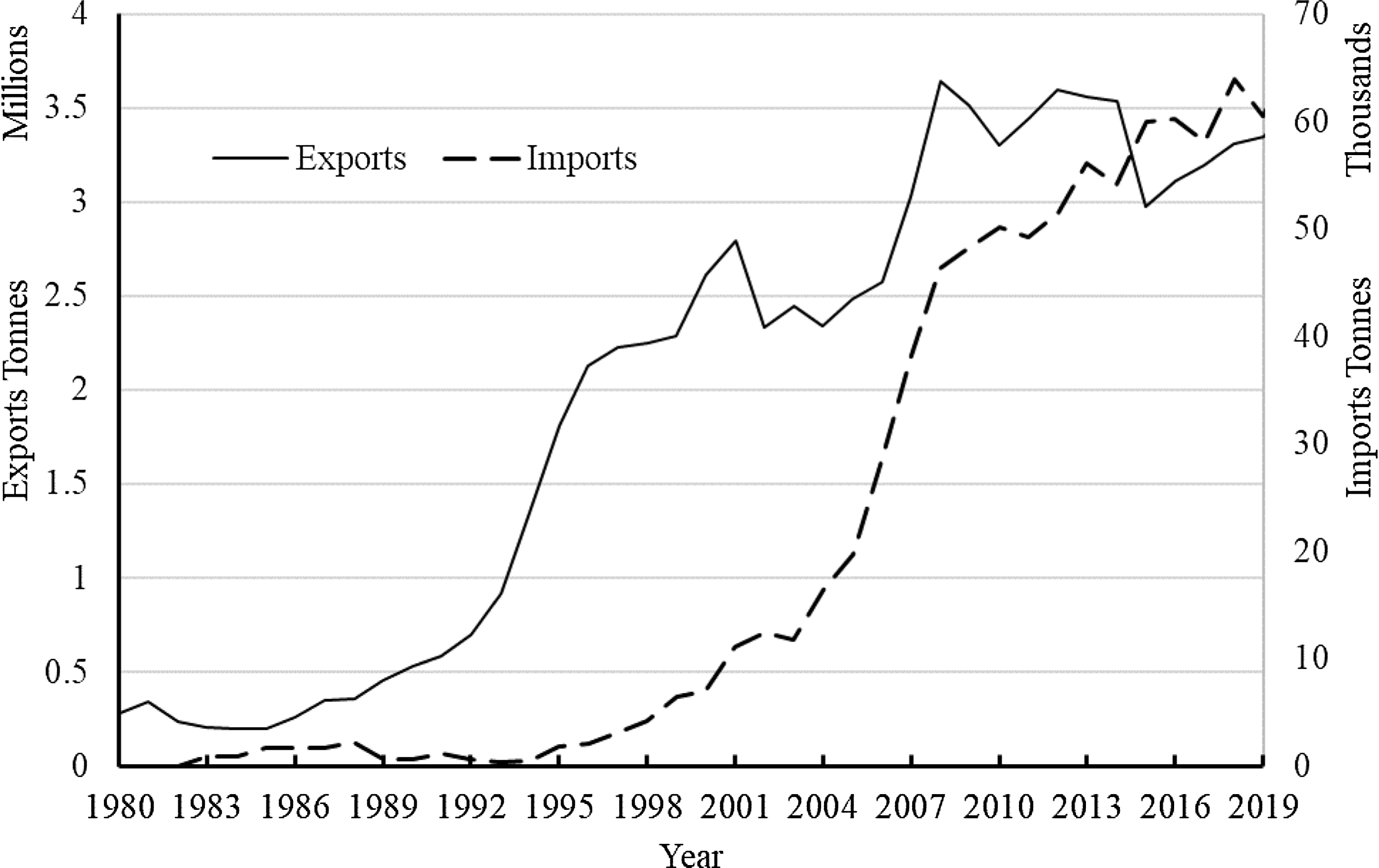
Production has also undergone changes. Percentage increases in production mirror the change in consumption, increasing over time but experiencing a slowdown starting around 2000 (Figure 2). Changes in production among the states between 1980 (first year of the data used in this study) and 2019 (last year) are shown in Figure 3. One can see an increase in production between the years and a shift in production toward southern states. Poultry production is the most vertically integrated agricultural production sector in the USA with production becoming more concentrated both in regionally and in the number of firms involved (Goodwin, Reference Goodwin2005; Hendrickson, James, and Heffernan, Reference Hendrickson, James and Heffernan2018). Broilers represent about 70% of poultry production value with these birds are sold as whole chickens or further processed to cut parts (Weersink et al., Reference Weersink, von Massow, Bannon, Ifft, Maples, McEwan, McKendree, Nicholson, Novakovic, Rangarajan, Richards, Rickard, Rude, Schipanski, Schnitkey, Schulz, Schuurman, Schwartzkopf-Genswein, Stephenson, Thompson and Wood2021). Exports also show increases and changes around 2000, and imports around 2007 (Figure 4). Due to the bird flu, exports decreased in 2015 but imports continued their upward trend.

Figure 2. Annual total production of fresh or chilled meat from chickens along with year-over-year percent change in production.
Source: FAO (2022).

Figure 3. Production of broiler chicken by state in 1980 and 2019 (billions of heads).
Source: U.S. Department of Agriculture (2023).
Changes in consumption and production practices have led to changes in the poultry industry (Ollinger, MacDonald, and Madison, Reference Ollinger, MacDonald and Madison2005; Bouchard, Reference Bouchard2020; Martinez, Reference Martinez2019). Few studies, however, were found that looks at structural changes in the pricing of different retail chicken parts or whole birds. Further, those studies examining potential structural change in prices generally examined breaks in individual series and not the system. Bouchard (Reference Bouchard2020) using Bai–Perron tests for structural breaks find retail broiler monthly prices did not show a break, but both wholesale farm and Georgia dock prices indicate a break around May 2008. He then uses bivariate models to measure asymmetric responses to positive and negative price shocks in pre- and post-2008 finding asymmetries are not economically significant regardless of period. Martinez (Reference Martinez2019) using chicken parts prices from April 2003 to February 2019 finds prices had three structural breaks, 2007, 2011, and 2015. Results on structural breaks are from supremum Wald tests. He hypotheses the 2007 and 2015 breaks are due to supply changes and the 2011 break coincides with the worldwide recession. Further, Martinez (Reference Martinez2019) uses directed acyclic graphs (DAGs) to provide better understanding on meat price relationships. His study suggests relationships between chicken part prices have changed over time and should be accounted for in analyzing demand for meat.
Taking a different approach, MacLachlan and Boussios (Reference MacLachlan and Boussios2018) estimate a vector autoregression (VAR) containing production, storage, and prices for broilers and qualitative variables for disease outbreaks in 2004 and 2014–2015. They also estimate a regime shifting model, which does not explicitly consider breaks. They conclude at the national level the broiler market is resilient, which can handle negative shocks, and VECM models may more accurately characterize the system. As expected, studies also indicate COVID-19 impacted the poultry industry (Ramsey et al., Reference Ramsey, Goodwin, Hahn and Holt2021; Weersink et al., Reference Weersink, von Massow, Bannon, Ifft, Maples, McEwan, McKendree, Nicholson, Novakovic, Rangarajan, Richards, Rickard, Rude, Schipanski, Schnitkey, Schulz, Schuurman, Schwartzkopf-Genswein, Stephenson, Thompson and Wood2021).
2.2. Law of one price
Arbitrage ensures markets will have one price net of transaction costs (transportation and trading). Within time series analysis, this law is often modeled using cointegration analysis. The basic idea is that nonstationary time series move toward a long-run equilibrium (Engle and Granger, Reference Engle and Granger1987). Using this idea, Awokuse and Bernard (Reference Awokuse and Bernard2007) estimate a VECM to investigate integration of U.S. four regional broiler prices for the years 1991–2002 prices. They note “… no previous study had specifically investigated the nature of market integration for regional broiler markets” (Awokuse and Bernard, Reference Awokuse and Bernard2007, p. 455). Findings include the four regional prices are integrated in the long run but pairwise cointegration is not present, indicating the law of one price may not hold. Consistent with Awokuse and Bernard (Reference Awokuse and Bernard2007), Bouchard’s (Reference Bouchard2017) findings fail to identify the law of one price between regional broiler prices.
Oh-Bok (Reference Oh-Bok2002), using monthly data from January 1990 to January 2001, estimates a VAR to examine relationship between U.S. and Korean wholesale chicken prices. He finds no evidence of structural change in Korean prices, but the U.S. adjusted price by the Korean exchange rate shows a change due to the 1997 Korean financial crisis. Impulse response and forecast error variances are then estimated for two regimes, January 1990 to December 1996 and January 1997 to January 2001. He concludes the markets are integrated and shocks occurring outside Korea impact the Korean market. In another study testing integration between two countries, Vollrath and Hallahan (Reference Vollrath and Hallahan2006) find the national markets in the USA and Canada for whole chickens are segmented. They suggest this finding is because poultry supply is managed in Canada; in particular, Canada upholds tariff-rate quotas on imports to ensure the effectiveness of its domestic poultry program.
Haghighat and Abdolahi (Reference Haghighat and Abdolahi2011) find chicken product markets in Iran provinces are integrated; the markets are individual markets in the short run but are a single market in long run. Ghahremanzadeh (Reference Ghahremanzadeh2015) concludes the law of one price holds for seven broiler pairs in Iran. He finds nonlinear behavior existence in the markets using an exponential smooth transition autoregressive model. Given the importance of the poultry/broiler industry, one would expect more studies on regional pricing in the USA like the two above studies. The market structure, however, limits market transaction data (lack of competitive markets) necessary for such analysis.
3. Data
Monthly retail prices per pound for fresh whole chickens from January 1980 to December 2019 for the Northeast, South, Midwest, and West regions are obtained from U.S. Bureau of Labor Statistics (2022). Average consumer prices are calculated from prices collected for the consumer price index. Monthly prices are collected by Bureau of Labor Statistics for 75 urban areas (U.S. Bureau of Labor Statistics, 2023a). Retail prices are for whole, fresh, and boiler/fryer chickens, which include organic and non-organic. Sufficient sample size allows average prices to be calculated for the four major census geographic regions: Northeast, Midwest, South, and West. A list of states in each region is provided in Table 1. As noted for brevity, chicken is used to refer to the retail prices.

Data after 2019 are excluded to eliminate price fluctuation due to the COVID-19 and the large number of missing values especially for the Northeast region. During 1980–2019, the West, Midwest, and South regions had no missing values, while the Northeast region had seven missing values. Based on the assumption of random walk, missing values are replaced by the previous month’s price. Previous studies such as Park, Mjelde, and Bessler (Reference Park, Mjelde and Bessler2008), Olsen, Mjelde, and Bessler (Reference Olsen, Mjelde and Bessler2015), and Duangnate and Mjelde (Reference Duangnate and Mjelde2020) have used the random walk assumption to replace missing values. As shown in Figure 5, prices show an upward trend. Variability in and the spread between prices also appears to increase over time. Over the entire data, prices show no seasonality. In regressing each series on monthly or seasonal qualitative variables, no coefficients are significant at the 5% level with the smallest p-value being 0.53.

Figure 5. Monthly fresh whole broiler price per pound by region, not seasonally adjusted.
Source: U.S. Bureau of Labor Statistics (2022).
Remaining analyses are conducted using the natural logarithm of each series. Augmented Dickey–Fuller tests suggest each series is nonstationary in levels, but first differences are stationary (since the tests are all the same inference for brevity, Augmented Dickey–Fuller statistics are not presented).
4. Methodology
One strength of the VECM and DAGs methodology is the methodology allows for the examination of price relationships at different time lengths: contemporaneous time (DAG), short term (number of lags), and longer term (cointegration). Innovation-accounting techniques are then used to examine the combined impacts of the different time lengths. The flexibility of the methodology allows the relationships to vary by time length such that a relationship seen at one-time length may differ at another length.
Because all price series are nonstationary in levels but stationary in first differences, a VECM is an appropriate framework to examine retail price dynamics in the U.S. chicken market. A VECM is
 $$\Delta P_{t}=\mu +\Pi P_{t-1}+\sum _{i=1}^{k-1}\Gamma _{i}\Delta P_{t-i}+e_{t},$$
where P
t
is a (4 × 1) vector of the four regional chicken prices, ΔP
t
denotes the first difference of P
t
, and μ is a (4 × 1) vector of constants. ΠP
t − 1 is the error correction term, where Π is a matrix of coefficients and P
t − 1 is a (4 × 1) vector of lagged prices of order one. $\Gamma _{{i}}$
is a matrix of coefficients corresponding to lagged first-differenced prices of order i, k is an integer indicating the lag order of the VAR model, and e
t
is a vector of innovations (Hansen and Juselius, Reference Hansen and Juselius1995). Note, a kth order VAR corresponds to a k−1th order VECM. Rewriting Π = αβ′ where α and β are both matrices of full rank (four in our case for the four regions) and the number of cointegrating vectors is less than four, the long-run relationship is identified by the cointegration space spanned by β while the short-run structure is identified through α and Γ
i
(Johansen, Reference Johansen1995).
$\Gamma _{{i}}$
is a matrix of coefficients corresponding to lagged first-differenced prices of order i, k is an integer indicating the lag order of the VAR model, and e
t
is a vector of innovations (Hansen and Juselius, Reference Hansen and Juselius1995). Note, a kth order VAR corresponds to a k−1th order VECM. Rewriting Π = αβ′ where α and β are both matrices of full rank (four in our case for the four regions) and the number of cointegrating vectors is less than four, the long-run relationship is identified by the cointegration space spanned by β while the short-run structure is identified through α and Γ
i
(Johansen, Reference Johansen1995).
4.1. Diagnosing parameter non-constancy
Tests employed in previous studies examining chicken prices are conducted on each individual price series and not the system. Rather than examining each series separately, tests which jointly examine all series are used. The test is Hansen and Johansen (Reference Hansen and Johansen1999)’s test, which examines if the VECM system’s parameters remain constant over time. To conduct these tests, a base sample is necessary to estimate the first VECM. Then two versions of the test, the X-form and the R-form, are obtained by recursively estimating the VECM adding one observation at time. In the X-form model, all parameters are re-estimated allowing all parameters to vary over time, whereas in the R-form model, the constancy of VECM parameters is analyzed given that the short-run dynamics are constant over time (Hansen and Johansen, Reference Hansen and Johansen1999). The test is a supremum test based on recursively estimated eigenvalues, which is a conservative test of the constancy of the parameters (Juselius, Reference Juselius2006).
4.2. Innovation accounting techniques
Innovation accounting techniques including impulse response functions (IRFs) and forecast error variance decompositions (FEVDs) are used to analyze dynamic responses between regional chicken prices. IRFs demonstrate how broiler prices respond to a one-time shock in the prices in one of the regions. FEVDs quantify how the forecast error for each price at any time is decomposed into innovations of the four prices (Doan, Reference Doan2000). Specifically, FEVDs give the percentage of price variation attributed to each market’s innovations at time t (Park, Mjelde, and Bessler, Reference Park, Mjelde and Bessler2008).
In Equation (1), the independence of the innovations, e t , is imposed but contemporaneous correlation is not restricted. The existence of contemporaneous correlation may cause innovative accounting techniques to provide meaningless results. To obtain contemporaneously uncorrelated innovations, e t is orthogonalized. The observed innovations, êt, are modeled as
 $$\hat{e}_{t}=A^{-1}\varepsilon _{t},$$
where ϵ t is a vector of underlying sources of variation, which are orthogonal to other sources of variation and A is a matrix representing how each non-orthogonal innovation is caused by the orthogonal variation in each equation (Bernanke, Reference Bernanke1986). To obtain Equation (2), DAGs are used to identify contemporaneous causal flows among the four regional broiler prices.
4.3. Directed acyclic graphs
DAGs provide a way to summarize the contemporaneous causal flows to provide a Bernanke ordering (Park, Mjelde, and Bessler, Reference Park, Mjelde and Bessler2008). In a DAG, an arrow represents a causal flow exists between the two variables. For example, P i → P j indicates that P i causes P j . If there is no arrow connecting any two variables, information does not flow between the two variables. See Pearl (Reference Pearl2000) and Spirtes et al. (Reference Spirtes, Glymour and Scheines2000) for detailed discussions of DAGs. To obtain DAGs, a linear non-Gaussian acyclic algorithm (LiNGAM) within Tetrad (Center for Causal Discovery, 2023) is applied to the observed innovations. The DAGs are then used to specify the orthogonal innovations for the estimation of IRFs and FEVDs. LiNGAM overcomes issues induced by linear-Gaussian assumptions (Shimizu et al., Reference Shimizu, Hoyer, Hyvarinen and Kerminen2006).
5. Empirical results
5.1. Model diagnostics for the full data
Wang and Bessler’s (Reference Wang and Bessler2005) procedure is used here to simultaneously determine lag length (k) and the number of cointegrating vectors (r) by minimizing Hannan and Quinn’s (HQ) loss metric. For the VECM using the full dataset, 1980–2019, this measure is minimized at two lags and rank of two (for brevity, Hannan and Quinn metrics are not presented). Tests of “β equals a known β” of Hansen and Johansen (Reference Hansen and Johansen1999) are used to test for parameter constancy. Normalized X- and R-forms of the tests are graphed in Figure 6. By construction, the sequence of statistics converges to zero. If the test values of X(t) and R(t) are larger than 1, the null hypothesis of constancy is rejected, implying the beta parameters are not consistent with the beta parameters estimated using the full data. The large variability between the X(t) and R(t) observed in the beginning is due to the relatively small size of the base sample (Juselius, Reference Juselius2006). There appears to be a structural break around 2000. The constancy tests are reconducted using only the first half of the data, January 1980 to December 1999 as the base sample to check whether the estimated betas are the same as those of the latter half of the data, January 2000 to December 2019. In Figure 6, both the X(t) and R(t) values lie in the rejection region, suggesting the estimated betas differ between the two periods. Given these results and previous discussion, the remaining analysis is conducted for two periods, January1980 to December 1999 (pre-2000) and January 2000 to December 2019 (post-1999).

Figure 6. Results of Hansen and Johansen (Reference Hansen and Johansen1999) recursive tests of the constancy of parameters in the estimated VECMs.
5.2. Model specification: pre and post periods
Augmented Dickey–Fuller tests by period are the same as for the full dataset: levels are nonstationary, but the first differences are stationary. Again, following Wang and Bessler (Reference Wang and Bessler2005), the Hannan and Quinn loss metric is minimized with a lag length of two for both periods. Cointegrating rank, however, differs between the periods. For the pre-2000 period, a rank of two is found, whereas for the post-1999 period a rank of one is found. Chi-squared stationarity tests for the four-price series indicate all series are stationary within the VECMs at the 0.000 level or less. With four markets, one would expect three long-run relationships. Having less than three relationships may be due to the high level of vertical integration (see literature review on vertical integration) and production concentration in the poultry sector (see Figure 3).
5.3. Tests of variable exclusion and weak exogeneity
The null hypothesis of variable exclusion tests that a market is not included in the co-integration space is rejected at the 5% level by all markets except the Northeast in the pre-2000 period implying all markets except the Northeast are in the cointegration space (Table 2). Similarly, the null hypothesis of the weak exogeneity test is rejected by all markets except the Northeast. Inferences of the weak exogeneity tests are all markets except the Northeast respond to perturbations in the cointegration space or long-run equilibrium vectors. In the post-1999 period, exclusion tests indicate both the Northeast and South are not included in the cointegration space. Weak exogeneity tests indicate only the South and West respond to perturbations in the long-run equilibrium vectors at the 5% level. At the 7% level, however, all markets respond to perturbations. Based on these results and change in the number of cointegrating ranks, it appears that the law of one price holds only weakly for the four regional chicken prices.

5.4. Identifying contemporaneous structure
Causal flows suggested by LiNGAM with penalty discount of one are given in Figure 7. In the pre-2000 period, the Midwest market is an information sink; it does not provide information to any other markets. Information is provided by the South and West markets to the Midwest market. The South market is exogenous in contemporaneous time; no markets provide information to the South market. The Northeast market receives information from the South market, whereas the Western market receives information from both the South and Northeast markets. The post-1999 contemporaneous structure is simpler with only the South market providing information to the Northeast market in contemporaneous time.

Figure 7. Contemporaneous structure as given by the VECM innovations.
5.5. Forecast error variance decomposition
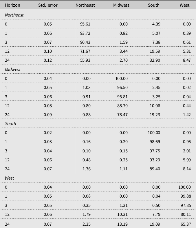
The question remains: do the differences in the VECM models translate into differences in how the models react to innovations in each series? To address this question, FEVD and IRFs are examined. FEVDs for each series in the two periods are presented in Tables 3 and 4. Listed are the decompositions at horizons 0 (contemporaneous time), 1, 3, 12, and 24 months ahead. FEVDs give the percentage of price variation in each market at each horizon due to an innovation in the market. For example, in contemporaneous time, uncertainty in Northeast market price in the pre-2000 period is explained by its own price (85.11%) and the South market (14.89%). At the 24-month horizon, Northeast prices are explained by itself (52.66%), Midwest (3.04%), South (25.40%), and West (18.91%). The other decompositions are interpreted in a similar fashion.
Table 3. Forecast error variance decompositions for four prices of fresh whole chickens of the pre-2000 period (January 1980–December 1999)

The entries are percentages, which sum to 100 for each row. The interpretation of each row is as follows: looking ahead at the horizon given in the far left-hand column (0, 1, 3, 12, or 24 months).
Table 4. Forecast error variance decompositions for four prices of fresh whole chickens of the post-1999 period (January 2000–December 2019)
The entries are percentages, which sum to one hundred for each row. The interpretation of each row is as follows: looking ahead at the horizon given in the far left-hand column (0, 1, 3, 12, or 24 months).
In the pre-2000 period for contemporaneous time, each market’s own price explains a sizable percentage of price variation, ranging from 64% in the Midwest market to 100% in the South market. A large percentage of own price explaining its market price variation remains for 24-month horizon in the Northeast, South, and West markets; approximately 50% or more of the variation being explained by its own price. The Midwest price explains only 20% of the variation in its own price at the 24-month horizon. Besides own price, the South market is the most important market in explaining prices for the first year. After the first year, the West market slightly overtakes the South market in percentages in the Midwest market. In every market, the South market quickly explains (month 3 or less) over 30% of price variations. No market appears to be exogenous as at least one other market explains a large percentage of the variation.
For the Northeast market, its own price explains 85% of its price variation at contemporaneous time decreasing to 53% at the 24th month. The South market in contemporaneous time explains 15% of the variation in price but increases to 28% by the first month and stays near that percentage for the first year. The West market explains a small percentage at the early horizons but increases to 19% by the 24th month. Own price in the Midwest market explains 64% of price variation in contemporaneous time but decreases to 43% by the first month and continues to decrease to 20% by the 24th month. The South market percentage in explaining Midwest price variation starts at 32% increases to 49% by the third month and then decreases to 33% by the 24th month. The West market increases in importance in explaining Midwest price variation increasing from 4% to 39%, whereas the Northeast explains no more than 7.5% at any horizon. Given the percentages of variation explained by other markets, the Midwest is the most endogenous market. Own price and the West market explain 87% or more of variation in South’s market price at all horizons with own price explaining more that 56% at every horizon. In explaining South’s market price, the Midwest is slightly more important than the Northeast but the combination of these two markets is never greater than 13%. The West market price variation is explained primarily by its own price and the South Market’s price. Northwest and Midwest prices increase in importance with their combined percentages increasing from 4% in contemporaneous time to over 19% by the 24th month.
Inferences change for the post-1999 period. For all markets, the importance of own price increases at every horizon increasing the exogenous nature of each market. At 1 year, the percentage of own price explaining price variability is 73% or larger in each market. At the 24th month, this increase in own market importance is particularly observable in the Midwest, South, and West markets. Similar to the pre-2000 period after own price, the South market’s is generally the most important in explaining price variation in all markets post-1999. The Northeast plays almost no role in any market other than itself.
In the Northeast market, own price increase importance is associated with a decrease in the importance of both the South and West markets for the first year. The South market increases in importance beginning in the second year. The largest changes occur in the Midwest market where own price now explains 78% or more of its own price variation at all horizons. This increase in importance of own price is associated with a decrease in importance of the three other markets with the Northeast and West playing little to no part in explaining price variability. South market price explains only a small amount of Midwest price variation until approximately 1 year. South market explains over 89% of its own price variability at all horizons. Northeast and Midwest play little to no part in explaining South’s price variation, the West plays a minor role at less than 8% at all horizons. The increase in importance of own price in the West market is accompanied by decreasing importance in the Northeast and South markets. The importance of the Midwest market shows a slight increase. The FEVDs show all the markets are more exogenous in the post-1999 period than in the pre-2000 period with the South and Midwest becoming almost completely exogenous. In both periods, after 12 months the FEVDs change little.
5.6. Impulse response functions
IRFs are presented as a matrix of graphs in Figure 8. Graphs represent the response of each market to a one-time innovation in a market along upper and lower bounds represented by 0.16 and 0.84 quantiles based on 1,000 simulations. Axes on individual graphs are normalized responses on the y-axis and months on the x-axes. Normalization allows for comparison among the markets. The market that is shocked is given by the market listed at the top of each column and responses by the market listed in each row.

Figure 8. Impulse response functions and upper and lower bounds given by 0.16 and 0.84 quartiles.
In the pre-2000 period, shocks in all markets cause a positive response in all other markets with the responses being significant as given by the upper and lower bounds not including zero at least initially. Zero is not included in all responses except for Northeast’s responses to a shock in the Midwest market at later horizons. Further, the system is stable as the responses are not exploding. Initial responses are the largest for shocks in their own market. Responses to shocks in the South market are the next largest responses after innovations to own price. This is in line with FEVDs indicating the importance of the South market in explaining price variation in other markets. Magnitudes of the responses to a shock in the West market are the third largest after the responses to shocks in the South market. Responses to shocks in the Northeast and Midwest markets are similar in the South and West markets.
As in the pre-2000 period, responses to own shock in all markets remain the largest responses in terms of magnitude in the post-1999 period. Similarly, the second largest responses belong to shocks in the South market. In contrast to the pre-2000 period, in the post-1999 period some point estimates for the responses are negative. In all cases except one, zero is inside the upper and lower bounds bands if the point estimate is negative. The exception is Northeast responses to a shock in the Midwest market. Responses in the Northeast market are positive and significant to shocks in the Northeast, South, and West markets. Significant Midwest market responses are found to shocks in Midwest and South prices. The South market significantly responses to shocks in itself and the West market. Significant responses are found in the West market to shocks in all markets.
6. Discussion and conclusions
Background information and results support the idea that structural changes have taken place over time in the broiler sector. Hansen and Johansen (Reference Hansen and Johansen1999)’s tests suggest that chicken pricing relationships among the four regional markets changed around 2000. Increases in production and consumption, changes in exports, and a shift in production toward southern states are postulated as causes of the structural change in retail prices. Increasing per capita chicken consumption slowed down in the early 2000s but resumed after 2017. Export volumes during the post-1999 appeared to be more volatile than those during the pre-2000. Future studies should be conducted to determine the causes of any structural change(s) and how much of the change(s) can be attributed to each factor.
Taken in their entirety, results from the various time lengths indicate some level of integration among the four retail markets; however, the level of integration has decreased between pre-2000 and post-1999 periods. The markets are becoming more exogenous. This decrease in integration is observed at the different time lengths. In contemporaneous time, in the pre-2000 period, Midwest, South, and West markets provide information for price discovery, but post-1999 only the South market provides information. The short term may have seen the smallest change, at least in the terms of the optimal lag length which did not change between periods, although coefficient magnitudes change. Longer term saw a decrease in the number of cointegrating vectors from two to one. Variable exclusion and weak exogeneity tests reveal that in the pre-2000 period all markets except the Northeast are in the co-integration space and respond to perturbations in the long-run equilibrium, whereas, in the post-1999 period, neither the Northeast nor the South is in the co-integration space. Weak evidence (7% level) exists that all markets respond to perturbations in the post-1999 period. FEVD and IRFs, which combine the effects of the different time lengths, show an increasing importance of each own market in explaining price variation and decreasing responses to innovations in other markets in the post-1999 compared to the pre-2000 period.
Cointegrating vectors imply price information in one regional market is transmitted to the other markets in the long run. The level of integration, however, is less than one may expect in an efficiently functioning market. Agricultural markets for grains and other meats appear to be more highly integrated. Being less integrated than other commodity markets may be due to the high level of vertical integration and production concentration in the poultry sector. Another factor is the highly perishable nature of fresh chickens with a need to maintain cold temperatures for transport and storage. This aspect increases transportation costs over other commodities on a per unit basis. Chickens, for example, are often transported in ice which increases weight, therefore, transportation costs. Another difference is examining retail instead of wholesale prices. Obviously, less movement occurs with products placed in retail stores than at the wholesale level.
Beyond the scope of this study is determining how the decrease in level of integration impacts overall market efficiency. It appears at the retail level, the law of one price only weakly holds. The South market is the most important market for price discovery in either period. The importance of the South market may be explained by the concentration of production in southern states. Less efficient markets may lead to a decrease in society’s welfare. Studies are necessary to examine this question considering transaction costs including transportation costs.
Data availability statement
Publicly available datasets were analyzed in this study. Monthly retail price per pound for fresh whole chickens for the Northeast, South, Midwest, and West regions is obtained from U.S. Bureau of Labor Statistics (2022). Monthly consumer price index is collected by Bureau of Labor Statistics for 75 urban areas (U.S. Bureau of Labor Statistics, 2023a). The data are available from the authors.
Author contribution
Conceptualization, J.W.M. and K.D.; methodology, J.W.M. and K.D.; formal analysis, J.W.M. and K.D.; data curation, J.W.M. and K.D..; writing – original draft, J.W.M. and K.D.; writing – review and editing, J.W.M. and K.D.; funding acquisition, n/a.
Financial support
This research received no specific grant from any funding agency, commercial, or not-for-profit sectors.
Competing interests
Kannika Duangnate and James Mjelde declare none.


 Open access