


1. Introduction
Modelling turbulence dissipation is fundamental for turbulence modelling. Turbulence models that aim to predict spatio-temporal variations of turbulent flow fields, such as large eddy simulations, ideally require non-homogeneous and dynamic models of the turbulence dissipation. This makes relations such as
 \begin{equation} \varepsilon = C_\varepsilon K^{3/2} / L \end{equation}
very relevant, particularly if such a relation can capture space and/or time variations of the turbulence dissipation rate  $\varepsilon$, and of related quantities such as a turbulent kinetic energy $K$, and an integral length scale $L$ characterising the largest, energy-containing, eddies. According to Kolmogorov's equilibrium cascade for homogeneous turbulence, the dimensionless dissipation rate coefficient $C_\varepsilon$ is constant at a large enough Reynolds number, i.e. independent of time, space and Reynolds number. Even though this is true in statistically stationary forced homogeneous turbulence after averaging over time, it is not true generally. There are significant variations of $C_\varepsilon$ both in space and in time in a variety of turbulence flows with close to $-5/3$ power-law energy spectra, and these variations obey well-defined laws. For example, in three qualitatively different turbulent wake flows generated by pairs of side-by-side square prisms, Chen et al. (Reference Chen, Cuvier, Foucaut, Ostovan and Vassilicos2021) showed that the dissipation rate coefficient of the incoherent turbulence varies along the cross-stream direction as $( \sqrt {Re_C} / Re_\lambda )^{3/2}$, where $Re_C$ is a Reynolds number based on the characteristic size and energy of the large-scale coherent structures, and $Re_{\lambda }$ is a local Taylor-length-based Reynolds number. These are cases of spatial variations of the dissipation rate coefficient after averaging over time, but similar conclusions have been reached for time variations after averaging over space. For example, it has been shown by Goto & Vassilicos (Reference Goto and Vassilicos2015, Reference Goto and Vassilicos2016a) that the time fluctuations of $C_\varepsilon$ are anti-correlated with those of the Taylor-length-based Reynolds number in forced homogeneous/periodic turbulence. In fact, for high enough Reynolds numbers, they showed that these time fluctuations closely follow $C_\varepsilon \sim ( \sqrt {Re_G} / Re_\lambda )^{n}$ (where $Re_G$ is a global Reynolds number, and $Re_{\lambda }$ the local (in time) Taylor-length-based Reynolds number) with $n=1$, and they demonstrated that this relation characterises non-equilibrium (i.e. non-Kolmogorov) cascades. Such a relation is also present in various decaying turbulent flows, such as decaying periodic turbulence simulated by direct numerical simulations (DNS) (Goto & Vassilicos Reference Goto and Vassilicos2016b) where the turbulence decays in time, but also in turbulent flows where the turbulence decays along the streamwise direction, such as grid-generated turbulence, turbulence jets and various turbulent wakes of bluff bodies; see Vassilicos (Reference Vassilicos2015), Cafiero & Vassilicos (Reference Cafiero and Vassilicos2019) and Chongsiripinyo & Sarkar (Reference Chongsiripinyo and Sarkar2020). Ortiz-Tarin, Nidhan & Sarkar (Reference Ortiz-Tarin, Nidhan and Sarkar2021) exceptionally found $n=4/3$ for the turbulent wake of a slender rather than bluff body because of an important difference in large-scale coherent structures compared to the bluff bodies of the previous studies.
With the exception of Nedić, Tavoularis & Marusic (Reference Nedić, Tavoularis and Marusic2017) and Obligado et al. (Reference Obligado, Brun, Silvestrini and Schettini2022), there has been little work to date on the spatio-temporal variations/fluctuations of turbulence dissipation, and in particular  $C_{\varepsilon }$ and $Re_{\lambda }$, in wall-bounded flows. In view of the general importance of turbulence dissipation dynamics and profiles for turbulent flow modelling, it is essential to study them in a wall-bounded turbulent flow. In this paper, we focus on the fully developed statistically stationary turbulent channel flow, specifically in the region of the flow where there is approximate time-average equilibrium between production and dissipation. Similarly to forced statistically stationary and homogeneous turbulence, this channel flow is also a forced statistically stationary turbulent flow, and similarly to the DNS of forced periodic turbulence of Goto & Vassilicos (Reference Goto and Vassilicos2015, Reference Goto and Vassilicos2016a), one expects dissipation rate coefficients and the local (in time) Reynolds numbers to also fluctuate in time in DNS of statistically stationary turbulence channel flow. Do they fluctuate in a similarly anti-correlated way as in forced homogeneous turbulence where these fluctuations result from the turbulence cascade? DNS of statistically stationary fully developed turbulent channel flow is a natural next step from DNS of statistically stationary periodic turbulence as they have two rather than three periodic directions and one wall-normal direction, which is non-homogeneous. One can therefore use DNS of such a flow to study the scalings of turbulence dissipation rate both in time, as already mentioned, and also in a cross-stream direction along which the turbulence is non-homogeneous, namely the turbulent channel flow's wall-normal direction. Are the wall-normal variations of turbulence dissipation rate and of local (in space) Reynolds number somehow related, and does such a relation have some commonalities to the way they are related in other non-homogeneous turbulent flows? These are universal questions that can be asked for any turbulent flow as they concern spatio-temporal variations of turbulence dissipation, turbulent kinetic energy and various length scales. These questions are central for future developments of turbulence subgrid modelling approaches, and in this paper, we ask them for turbulent channel flow.
In the next section, we present the DNS data of statistically stationary fully developed turbulent channel flow used in this study. Then, in § 3, we study the cross-stream variations of the time- and wall-parallel plane-average values of  $C_{\varepsilon }$ and $Re_{\lambda }$ in the average equilibrium layer where turbulence production rate approximately balances dissipation rate. In § 4, we remove the time-averaging operation and study the time dynamics of the wall-parallel plane-average values of $C_\varepsilon$ and $Re_\lambda$. Finally, we conclude in § 5.
Note that the notation used in the remainder of this paper has some subtle differences from the notation used in this Introduction, where it has been possible to include only summary descriptive sketches of previous results.
2. DNS data
Our analysis is comprised of two parts. In the first part, we analyse the mean profiles of various quantities in the wall-normal direction (i.e. functions of wall-normal coordinate  $y$) for a turbulent channel flow. Our primary database consists of the DNS data of Lee & Moser (Reference Lee and Moser2015) for four cases with $Re_\tau =550$, 1000, 2000 and 5200 ( $Re_{\tau } \equiv u_{\tau } \delta /\nu$, where $\nu$ is the kinematic viscosity, $\delta$ is the channel half-width, and $u_{\tau }$ is the skin friction velocity obtained by averaging over time and over streamwise coordinate $x$ and spanwise coordinate $z$ at the channel's solid wall $y=0$). The Navier–Stokes equations have been solved by integrating the evolution equations in terms of the wall-normal vorticity and the Laplacian of the wall-normal velocity for an incompressible fluid. The spatial discretisation in the wall-parallel directions used the Fourier spectral method, whereas a B-spline collocation method was used in the wall-normal directions. For the time advancement, a third-order Runge–Kutta method for the nonlinear terms and a Crank–Nicolson method for the viscous terms were selected. The domain size is $L_x=8{\rm \pi} \delta$ and $L_z=3{\rm \pi} \delta$.
For our second part, we focus on the time dynamics of turbulence again in a channel flow, and therefore we use the DNS data of Lozano-Durán & Jiménez (Reference Lozano-Durán and Jiménez2014) for  $Re_\tau =932\ \textrm {and}\ 2003$, where the full velocity field is available with a time resolution of $dt^+\approx 8$ for $Re_\tau =932$ and total number of time steps $N_t=3151$, and $dt^+\approx 25$ for $Re_\tau =2003$ with $N_t=462$, while the domain size for both simulations is $L_x=2{\rm \pi} \delta$ and $L_z={\rm \pi} \delta$ (the superscript $^+$ refers to non-dimensionalisation with wall units). The numerical methodology is similar to that of Lee & Moser (Reference Lee and Moser2015), except for the spatial discretisation in the wall-normal direction. For $Re_\tau =932$, Chebyshev polynomials were used, while $Re_\tau =2003$ used a seven-point compact finite difference scheme. Finally, a third-order semi-implicit Runge–Kutta method with Courant–Friedrichs–Lewy coefficient 0.5 was chosen for time advancement. A detailed comparison of the two datasets can be found in table 1, along with the naming convention that will be followed in the following sections.
Table 1. DNS databases.

3. Time-averaged turbulence dissipation scalings
In this section, we analyse the dataset of Lee & Moser (Reference Lee and Moser2015). All the quantities have been averaged over the two homogeneous directions, i.e. over the  $x,z$ plane, and over time. We therefore look at profiles in the wall-normal direction $y$. Townsend (Reference Townsend1961) proposed that for high Reynolds numbers, there is an inertial layer $\delta _\nu \ll y \ll \delta$ ( $\delta _\nu \equiv \nu / u_\tau$) where production rate and dissipation rate (both averaged over the homogeneous plane at a fixed $y$ and over time) are in equilibrium. This idea received support from the asymptotic analysis of Brouwers (Reference Brouwers2007), which, however, started from the assumption that the mean flow profile is logarithmic in that region. In figure 1(a), we plot the ratio between turbulent kinetic energy production rate $\bar {\mathcal {P}} \equiv -\overline {\langle uv\rangle }({{\rm d} U}/{{\rm d}y})$ (where $\langle uv\rangle$ is the Reynolds shear stress obtained by averaging over the $x,z$ plane at $y$ at time $t$, and $(U,0,0)$ is the mean flow obtained by averaging over that plane and time) and dissipation rate $\bar {\varepsilon }$ (where $\varepsilon$ is the turbulence dissipation rate averaged over that same plane, and the overline represents an average over time). We observe that this ratio oscillates gently around 1 over an increasing wall distance range with increasing $Re_{\tau }$. Our analysis is focused on the region above the buffer layer, starting from $y/\delta _{\nu }\equiv y^+ \approx 60$ where $\bar {\mathcal {P}}/\bar {\varepsilon }$ displays a local minimum irrespective of Reynolds number, and ending at the wall distance $y^+\approx 0.5Re_\tau$ where the ratio of production over dissipation suddenly drops fast for all $Re_{\tau }$ cases. In this region, there is also a local maximum of $\bar {\mathcal {P}}/\bar {\varepsilon }$ that appears relevant for the $y$-range of validity of some of our results in the following subsections. This local maximum may either be a finite Reynolds number effect or indicate that the location of the local maximum of $\bar {\mathcal {P}}/\bar {\varepsilon }$ is a fundamental differentiating factor in the physics of wall turbulence. Either way, it is important to analyse the entire $y$-region where $\bar {\mathcal {P}}/\bar {\varepsilon }$ oscillates close to 1, and distinguish subregions within it. In § 3.1, we examine wall-normal profiles of the Taylor length because of its relation to turbulent kinetic energy and turbulence dissipation rate, and because it is the length scale used to define the Taylor-length-based Reynolds number. In § 3.2, we study wall-normal profiles of integral length scales, and in § 3.3, we bring our length scale observations together and look at how dissipation rate coefficients scale with local Taylor-length-based Reynolds number along the wall-normal direction and, equivalently, how ratios of integral to Taylor length scales vary with normalised wall normal distance $y^{+}$ (which is also a local Reynolds number).

Figure 1. Mean profiles of: (a) production rate over dissipation rate of turbulent kinetic energy,  $\bar {\mathcal {P}}/\bar {\varepsilon }$; (b) Taylor length $\lambda$ normalised with $\delta _{\nu }$; (c) ratio between $-f\bar {K}/\overline {\langle uv \rangle }$, where $f(y^+, Re_\tau )=\bar {\mathcal {P}} / \varepsilon$, and the indicator function $\beta (y^+)=y^+({{\rm d} U^+}/{{{\rm d}y}^+})$; (d) Taylor-length-based Reynolds number $Re_\lambda \equiv \sqrt {\bar {K}\lambda }/\nu$. Colours indicate $Re_\tau =544$ (black lines), $Re_\tau =1000$ (blue lines), $Re_\tau =1994$ (green lines), and $Re_\tau =5186$ (orange lines). The thick part of a line corresponds to the region $60\le y^+ \le 0.5Re_\tau$, while the dots represent the local maximum of $\bar {\mathcal {P}}/\bar {\varepsilon }$.
3.1. Taylor length
Figure 1(b) shows the Taylor length, defined as  $\lambda \equiv \sqrt {10\nu \bar {K}/\bar {\varepsilon }}$, versus normalised wall distance $y^+$ (where $K = K(y,t)$ is the turbulent kinetic energy averaged over the horizontal $x,z$ plane, and $\bar {K}$ is $K$ averaged over time). As $Re_\tau$ grows, $\lambda$ tends towards $\lambda \sim \sqrt {\delta _{\nu } y}$ (in dimensionless form, $\lambda ^+\sim \sqrt {y^+}$) from the local minimum until the local maximum of $\bar {\mathcal {P}}/\bar {\varepsilon }$, while after that local maximum, it starts to deviate slightly from this scaling. From the definition of the Taylor length, this corresponds to a scaling $\bar {\varepsilon } \sim \bar {K} u_\tau / y$ for the turbulence dissipation. Similar results have been obtained by Dallas, Vassilicos & Hewitt (Reference Dallas, Vassilicos and Hewitt2009), who predicted $\lambda \sim \sqrt {\delta _\nu y}$ on the basis of the number density of fluctuating velocity stagnation points, which scales as $1/y^{+}$ in the region where production approximately equals dissipation. It is worth noting here that the scaling of $\lambda$, and subsequently of $\bar {\varepsilon }$, has far-reaching consequences, even for statistics as basic as the mean velocity profile $U(y)$. In general, we can write
 \begin{equation} \left.\begin{gathered} \frac{\bar{\mathcal{P}}}{\bar{\varepsilon}} = f(y^+, Re_\tau), \\ -\overline{\langle u v \rangle} \frac{{\rm d} U}{{\rm d}y} = f \bar{\varepsilon} = f\,\frac{10\nu \bar{K}}{\lambda^2}. \end{gathered}\right\} \end{equation}
Using  $\lambda \sim \sqrt {\delta _\nu y}$, following our observation in figure 1(b), which suggests it to be increasingly the case as $Re_{\tau }$ increases, we obtain
 \begin{equation} \frac{{\rm d} U}{{\rm d}y} \sim \left[ \frac{10f\bar{K}}{-\overline{\langle uv \rangle}}\right] \frac{u_\tau}{y} \end{equation}
in the very high  $Re_{\tau }$ limit. Therefore, the consequence of $\lambda \sim \sqrt {\delta _\nu y}$ is that the quantity in brackets in (3.2) should vary with $y^+$ in the same way as the indicator function $\beta (y^+)=y^+({\textrm {d} U^+}/{{\textrm {d}y}^+})$. In figure 1(c), we plot the ratio between $-10f\bar {K}/\overline {\langle uv \rangle }$ and the indicator function. The ratio tends to become constant from $y^+\approx 60$ until the maximum of $\bar {\mathcal {P}}/\bar {\varepsilon }$ with increasing Reynolds number. This offers a different way to examine the extent to which the Taylor length's scaling remains valid, but also illustrates its relation to the mean shear scalings.
Another consequence of  $\lambda \sim \sqrt {\delta _\nu y}$ is that the eddy turnover time $\tau \equiv \bar {K}/\bar {\varepsilon }$ scales as $\tau \sim y / u_{\tau }$ in the inertial layer where production and dissipation are in approximate local equilibrium. It may be puzzling that $\tau$ scales with $1/u_{\tau }$ rather than $1/\sqrt {\bar {K}}$, as this eddy turnover time is often linked to the energy cascade. In § 4, we investigate turbulence dissipation time scales by lifting the time-average operation to study time scales in actual time fluctuations of quantities involving turbulent kinetic energy and dissipation.
3.2. Integral length scales
The integral length scale is the correlation distance of a fluctuating velocity component in a specific direction. It is typically interpreted as the size of the biggest eddies in a turbulent flow. In wall turbulence, due to the anisotropy imposed by the wall, these length scales have different magnitudes depending on the velocity component and direction of correlation. We calculate the integral length scales from (Tennekes & Lumley Reference Tennekes and Lumley1972)
 \begin{equation} E_{u_i u_i}(k_j=0) = \frac{2 \overline{\langle u_i^{2} \rangle}}{\rm \pi}\,L_{u_i, x_j}, \end{equation}
which relates the one-dimensional energy spectra to the integral length scales:  $i=1,2,3$ correspond to the three velocity components ( $u_1 \equiv u$, $u_2 \equiv v$, $u_3 \equiv w$) in the streamwise, wall-normal and spanwise directions, respectively, and $j=1,2,3$ correspond to the three directions ( $x_1 \equiv x$, $x_2 \equiv y$, $x_3 \equiv z$) along which correlations are measured. For example, for $i=2$ and $j=3$, we have $L_{v,z}$ representing the integral length scale of the wall-normal velocity in the spanwise direction, computed from the one-dimensional energy spectrum $E_{vv}(k_z)$. To invoke (3.3), the energy spectra must be well converged and present a plateau at the lowest wavenumbers. The one-dimensional energy spectra from the Lee & Moser (Reference Lee and Moser2015) dataset have such a plateau for $E_{vv}(k_z)$ and $E_{ww}(k_z)$ for all four Reynolds numbers and across the channel as shown in figures 2(d,f). The $E_{vv}(k_x)$ one-dimensional energy spectra in figure 2(b), associated with the streamwise structures, present a low-wavenumber plateau at all $y^+$ only for the lowest Reynolds number ( $Re_\tau =550$). For $Re_\tau \ge 1000$, the energy spectra remain constant at the lowest wavenumbers only up to a certain height above the wall, specifically up to $y^+\approx 200$, 300 and 500 for $Re_\tau =1000$, 2000 and 5200, respectively. This behaviour may be associated with the progressive appearance of very-large-scale motions (VLSMs) (Kim & Adrian Reference Kim and Adrian1999; Smits, McKeon & Marusic Reference Smits, McKeon and Marusic2011) as Reynolds number increases. Therefore, our analysis is focused on the three integral length scales $L_{v,x}$, $L_{v,z}$ and $L_{w,z}$, treating carefully, however, the results for $L_{v,x}$ above the $y^+$ limits just mentioned. Figures 2(a,c,e) show these integral length profiles in the wall-normal direction from $y^+\approx 60$ up to $y^+=0.5\,Re_\tau$. Here, $L_{v,x}$ tends towards a linear scaling with distance from the wall as $Re_\tau$ increases, especially for locations closer to the wall, where the spectra are constant at the lower wavenumbers. Also, $L_{v,z}$ shows very close to linear scaling with $y$, the exponent $0.9$ indicating perhaps that it has not yet reached its asymptotic value, which may require higher $Re_\tau$. Approximately, however, the present data provide some support for scalings of the type
 \begin{equation} L_{v,x} \sim L_{v,z}\sim y \end{equation}
at high enough  $Re_{\tau }$. These scalings are consistent with the attached eddy hypothesis of Townsend (Reference Townsend1976), where wall-normal fluctuations are dominated by eddy sizes comparable to the distance $y$ to the wall because of impermeability. The two integral length scales $L_{v,x}$ and $L_{v,z}$ seem to follow this scaling, and therefore may serve as characteristic dimensions of wall-attached eddies. Looking at figure 2(e), $L_{w,z}$ seems to scale with the square root of the distance from the wall, and the different Reynolds number curves show some tendency to collapse if we divide $L_{w,z}^+$ by the square root of $Re_\tau$, resulting in
 \begin{equation} L_{w,z}^+{\sim} \sqrt{Re_\tau\,y^+}\Rightarrow L_{w,z} \sim \sqrt{\delta y}\quad \textrm{i.e. } L_{w,z}/\delta \sim \sqrt{y/\delta}, \end{equation}
which suggests that  $L_{w,z}$ depends on $y$ and $\delta$. The scaling (3.5) is also in agreement with Townsend's phenomenology, in which eddies of size $y$ contribute to $v$ motions, whereas all eddy sizes equal to and larger than $y$ (up to $\delta$) contribute to $u$ and $w$ motions (Townsend Reference Townsend1976; Perry, Henbest & Chong Reference Perry, Henbest and Chong1986). The scaling (3.5) is new and, to the authors’ knowledge, has not yet been derived from Townsend's phenomenology or in any other way. (But see the last paragraph of § 3.3 below.)

Figure 2. (a,c,e) Integral length scales normalised with  $\delta _\nu$ as a function of wall distance for different $Re_\tau$; dots indicate the location of the local maximum of $\bar {\mathcal {P}}/\bar {\varepsilon }$. (b,d,f) Corresponding energy spectra normalised with $u_\tau ^2$ for different $y^+$ and $Re_\tau$. Plots show: (a) $L_{v,x}^{+}$ versus $y^+$, where the dashed line indicates a linear scaling $L_{v,x} \sim y$; (b) $E_{v,v}/u_\tau ^2$ versus $k_x$; (c) $L_{v,z}^{+}$ versus $y^+$, where the dashed line shows a scaling $L_{v,z}^{+} \sim y^{+^{0.9}}$; (d) $E_{v,v}/u_\tau ^2$ versus $k_z$; (e) $L_{w,z}^{+}/\sqrt {Re_\tau }$ versus $y^+$, where the dashed line indicates a square root scaling $L_{w,z} \sim \sqrt {\delta y}$; (f) $E_{w,w}/u_\tau ^2$ versus $k_z$. Darker to lighter colours correspond to increasing wall distances.
3.3. Range of scales for inertial energy cascade
In figures 3(a,c,e), we plot dissipation rate coefficients  $C_{\bar {\varepsilon }}^{u_i,x_j}\equiv \bar {\varepsilon } / (\bar {K}^{3/2}/L_{u_i,x_j})$ as functions of the local Taylor-length-based Reynolds number $Re_\lambda \equiv \sqrt {\bar {K}} \lambda /\nu$. Both $C_{\bar {\varepsilon }}^{u_i,x_j}$ and $Re_\lambda$ are based on statistics obtained by averaging over both time and $x,z$ planes, and their values vary as we move across the wall-normal direction $y$, in particular within the average equilibrium layer $60\le y^{+}\le Re_{\tau }/2$; see figure 1(d). We observe in figures 3(a,c) that $C_{\bar {\varepsilon }}^{v,x}$ and $C_{\bar {\varepsilon }}^{v,z}$ tend to a constant independent of $Re_\lambda$ as $Re_{\tau }$ increases, even though $Re_{\lambda }$ varies over an increasing range of values across the average equilibrium layer as $Re_{\tau }$ grows (figure 1d). This is different from the cross-stream non-homogeneous behaviour in turbulent wake flows generated by pairs of side-by-side square prisms where Chen et al. (Reference Chen, Cuvier, Foucaut, Ostovan and Vassilicos2021) found a $-3/2$ power-law dependence of a dissipation rate coefficient similar to $C_{\bar {\varepsilon }}^{v,x}$ on local Taylor-length-based Reynolds number. The cross-stream non-homogeneity scalings of turbulence dissipation seem, therefore, to be very different in the presence or absence of a wall.

Figure 3. (a,c,e) Dissipation rate coefficients  $C_{\bar {\varepsilon }}^{u_i, x_j}$ computed with different integral length scales versus $Re_{\lambda }$. (b,d,f) Wall-normal profiles of ratios $L_{u_i, x_j} / \lambda$. Plots show: (a) $C_{\bar {\varepsilon }}^{v,x}$ as a function of $Re_\lambda$; (b) $L_{v,x}/\lambda$ versus $y^+$, dashed line $y^{+^{0.5}}$; (c) $C_{\bar {\varepsilon }}^{v,z}$ as a function of $Re_\lambda$; (d) $L_{v,z}/\lambda$ versus $y^+$, dashed line $y^{+^{0.5}}$; (e) $C_{\bar {\varepsilon }}^{w,z}$ as a function of $Re_\lambda$, with inset $C_{\bar {\varepsilon }}^{w,z}$ premultiplied with $Re_\tau ^{-0.35}$; (f) $L_{w,z}/\lambda$ versus $y^+$, with inset $L_{w,z}/\lambda$ premultiplied with $Re_\tau ^{-0.35}$. Dots indicate the location of the local maximum of $\bar {\mathcal {P}}/\bar {\varepsilon }$.
The dissipation rate coefficient is, by definition, the ratio of the dissipation rate at the smallest scales to a rate  $\bar {K}^{3/2}/L_{u_i,x_j}$ characterising energy loss by the largest eddies. For $C_{\bar {\varepsilon }}^{v,x}$ and $C_{\bar {\varepsilon }}^{v,z}$, this ratio approaches a constant value in the average equilibrium range $60\le y^{+}\le Re_{\tau }/2$ as $Re_{\tau }$ increases, suggesting that the large-scale loss rate is the same fraction of dissipation rate at all these wall distances. For $C_{\bar {\varepsilon }}^{w,z}$, however, the situation is radically different. The time and wall-normal plane-averaged values of $C_{\bar {\varepsilon }}^{w,z}$ and $Re_{\lambda }$ vary with wall distance $y$, but they do so in an opposite way. Whilst $Re_{\lambda }$ grows with $y$,
$y$,  $C_{\bar {\varepsilon }}^{w,z}$ decreases with increasing $y$, and this is expressed by an approximate power-law scaling of a form close to $C_{\bar {\varepsilon }}^{w,z} \sim Re_\lambda ^{-1}$. If $C_{\bar {\varepsilon }}^{w,z}$ is independent of viscosity, then $C_{\bar {\varepsilon }}^{w,z} \sim Re_\lambda ^{-1}$ would require $C_{\bar {\varepsilon }}^{w,z} \sim \sqrt {Re_{\tau }}/Re_\lambda$, which is reminiscent of the non-equilibrium dissipation scaling mentioned in the Introduction, $Re_{\tau }$ being a global Reynolds number and $Re_{\lambda }$ being a local-in- $y$ Reynolds number. However, our data support a different, though close, relation $C_{\bar {\varepsilon }}^{w,z} \sim Re_{\tau }^{0.35}/Re_\lambda$, with a departure from $Re_{\lambda }^{-1}$ at the higher wall distances; see figure 3(e). This departure may be related to VLSMs. It cannot be known with the present data if the exponent $0.35$ tends to $0.5$ or not with increasing $Re_{\tau }$.
In homogeneous turbulence, the ratio of integral scale to Taylor length characterises the range of scales where the inertial energy cascade occurs (e.g. see Obligado & Vassilicos Reference Obligado and Vassilicos2019; Meldi & Vassilicos Reference Meldi and Vassilicos2021). In a turbulent channel flow, the anisotropy imposes different integral length scales in different directions, and even though all ratios  $L_{u_i,x_j} / \lambda$ can be defined in principle, it is not fully clear how each one of them may relate to a cascade mechanism. Even so, in figures 3(b,d,f) we plot the wall-normal profiles of $L_{v,x}/\lambda$, $L_{v,z}/\lambda$ and $L_{w,z}/\lambda$. From the asymptotic scalings $\lambda \sim \sqrt {\delta _\nu y}$ and $L_{v,x} \sim L_{v,z}\sim y$ suggested by our analysis in the previous section, we expect
 \begin{equation} L_{v,x}/\lambda \sim L_{v,z}/\lambda \sim \sqrt{y/\delta_\nu} \end{equation}
in the high  $Re_{\tau }$ limit. This is indeed consistent with what we observe in figures 3(b,d), in particular for higher $Re_{\tau }$ as the integral length scales and the Taylor length have not reached their asymptotic values for the small and medium $Re_\tau$ considered here. Note also that it is harder to compute $L_{v,x}$ accurately at the higher wall-normal locations, perhaps due to the potential emergence of large-scale motions as $Re_{\tau }$ increases. Relation (3.6) suggests that the range of eddy sizes where an inertial energy cascade affecting the wall-normal turbulence fluctuations is a priori conceivable, and increases with local Reynolds number $y^{+}$.
By doing the same analysis for  $L_{w,z}/\lambda$, i.e. from the asymptotic scalings $\lambda \sim \sqrt {\delta _{\nu } y}$ and $L_{w,z}\sim \sqrt {\delta y}$, we obtain
 \begin{equation} L_{w,z}/\lambda \sim \sqrt{Re_{\tau}} \end{equation}
in the high  $Re_{\tau }$ limit. Unlike $L_{v,x}/\lambda$ and $L_{v,z}/\lambda$, which are proportional to the square root of the local Reynolds number $y^+$, $L_{w,z}/\lambda$ is proportional to the square root of the global Reynolds number $Re_{\tau } = \delta ^{+}$. Looking at figure 3(f), we do indeed see approximate independence of $y$ and an increase of this constant with increasing $Re_\tau$. However, the different $Re_\tau$ curves collapse if we premultiply them with $Re_\tau ^{-0.35}$ (inset of figure 3f) rather than $Re_\tau ^{-0.5}$ as suggested by (3.7). Again, this discrepancy may be attributed to the low Reynolds numbers available here, making it difficult to see the correct asymptotic values of the quantities of interest. Nevertheless, it remains possible to argue that the range of scales contributing to $w$ fluctuations remains approximately constant with increasing distance from the wall in a significant portion of the approximate average equilibrium range of wall distances.
It is worth noting that (3.7), which is equivalent to  $C_{\bar {\varepsilon }}^{w,z} \sim \sqrt {Re_{\tau }}/Re_\lambda$, has significant predictive power. Using the facts that $L_{w,z}$ and $\lambda$ are, in all generality, functions of $y$,
$y$,  $\delta$ and $\delta _{\nu }$, and that we may expect $\lambda$ to be independent of $\delta$, and $L_{w,z}$ to be independent of viscosity in an approximate average equilibrium range, we can write $L_{w,z} = \sqrt {\delta y}\,f_{L}(y/\delta )$ and $\lambda = \sqrt {\delta _{\nu } y}\,f_{\lambda }(y/\delta _{\nu })$, where $f_L$ and $\,f_{\lambda }$ are dimensionless functions of dimensionless arguments. From (3.7), it then follows that $\,f_{L}(y/\delta )/\,f_{\lambda }(y/\delta _{\nu })$ is independent of $y$, which, given that $f_L$ is independent of $\delta _{\nu }$, and $\,f_{\lambda }$ is independent of $\delta$, is possible only if both $f_L$ and $\,f_{\lambda }$ are constants. Hence $\lambda \sim \sqrt {\delta _{\nu } y}$ and $L_{w,z}\sim \sqrt {\delta y}$, which demonstrates the predictive power of (3.7).
4. Non-equilibrium time-dependent dissipation scalings
Motivated by the eddy turnover time  $\tau \equiv \bar {K}/\bar {\varepsilon }$, which can be expected to scale as $\tau \sim y/u_{\tau }$ because $\lambda \sim \sqrt {\delta _{\nu } y}$ at high $Re_{\tau }$, and by the fact that this time scale is important for the scalings of the dissipation rate coefficients and the length scale ratios in the previous subsection, we now study fluctuations in time. We therefore lift the time averaging and study, at various wall-normal locations $y$, the time fluctuations of plane-averaged quantities, i.e. quantities averaged over the homogeneous directions in space $(x,z)$ but not over time. The purpose of this investigation is to find whether characteristic time scales exist in the time fluctuations themselves.
4.1. Time dynamics of dissipation rate coefficient  $C_\varepsilon$

For the second part of this work, we use the DNS data of Lozano-Durán & Jiménez (Reference Lozano-Durán and Jiménez2014) where full velocity fields have been stored for a large number of time steps; see § 2. For these data, integral length scales  ${\mathcal {L}}_{u_i,x_j}$ are obtained for $i=1,2,3$ and $j=1,3$ (we do not consider $j=2$) by first calculating autocorrelation functions where averages are in $x,z$ planes, and then integrating these autocorrelation functions up to the first zero crossing. These integral length scales are therefore functions of wall-normal distance $y$ and time $t$, unlike the integral scales $L_{u_i,x_j}$ obtained from energy spectra in the previous section, which are functions of $y$ but not of time $t$. Fluctuating dissipation coefficients are now defined as $C_\varepsilon ^{u_i,x_j}\equiv \varepsilon / (K^{3/2}/{\mathcal {L}}_{u_i,x_j})$, where $\varepsilon$ and $K$ are also functions of $y$ and $t$, and not functions of $y$ only. Note the difference between the fluctuating dissipation coefficients $C_\varepsilon ^{u_i,x_j}$ (functions of $y$ and $t$) and the non-fluctuating dissipation coefficients $C_{\overline \varepsilon }^{u_i,x_j}$ (functions of $y$ but not $t$). Similarly, we define a fluctuating Taylor length $\varLambda \equiv \sqrt {10 \nu K/\varepsilon }$ and a fluctuating Taylor-length-based Reynolds number $Re_{\varLambda } \equiv \sqrt {K} \varLambda /\nu$, which, unlike $\lambda \equiv \sqrt {10 \nu \bar {K}/\bar {\varepsilon }}$ and $Re_{\lambda } \equiv \sqrt {\bar {K}} \lambda /\nu$, are also functions of both $y$ and $t$.
$t$.
We plot in figure 4 the three fluctuating dissipation coefficients  $C_\varepsilon ^{v,x}$, $C_\varepsilon ^{v,z}$ and $C_\varepsilon ^{w,z}$ normalised by their standard deviation against the fluctuating local Reynolds number $Re_\varLambda$, also normalised by its standard deviation, for $Re_\tau =950$ at $y^+=193$, and for $Re_\tau =2000$ at $y^+=325$. For all three dissipation coefficients, we observe an apparently quasi-periodic behaviour consisting of turbulence-building periods, where the dissipation coefficient decreases and $Re_\varLambda$ grows, alternating with turbulence-declining periods, where the dissipation coefficient grows and $Re_\varLambda$ decreases. We must emphasise that this behaviour is not transient; indeed, it persists for the entire time duration of our data and it can also be found at all wall-normal locations in the range $60 \leq y^+ \leq 0.5\,Re_\tau$. This observation is similar to that made by Goto & Vassilicos (Reference Goto and Vassilicos2016a), who attributed it to the turbulence cascade and the resulting time lag between the forcing's energy build up and the dissipation's energy decrease in their DNS of periodic turbulence. Here, the role of the forcing is replaced by the mean shear, which creates large-scale turbulence, therefore increasing $Re_\varLambda$. The nonlinear cascade transfers energy towards the small scales, where turbulence activity is increased, thus increasing dissipation. These remarks raise the question of which time scale(s) govern these apparent quasi-periodicities, which we address in § 4.2.

Figure 4. Fluctuations in time of turbulence dissipation rate coefficients  $C_\varepsilon ^{u_i,x_j}$ and $Re_\varLambda$, for (a,c,e) $Re_{\tau }=950$ and $y^+=193$, and (b,d,f) $Re_\tau =2000$ and $y^+=325$. Grey lines in all figures show the time signal of $Re_\varLambda$, black lines in (a,b) show the time signal of $C_\varepsilon ^{v,x}$, blue lines in (c,d) show the time signal of $C_\varepsilon ^{v,z}$, and green lines in (e,f) show the time signal of $C_\varepsilon ^{w,z}$.
We quantify our observations by calculating the two-time correlation coefficients between  $C_\varepsilon ^{u_i, x_j}$ and $Re_\varLambda$, which are given by
 \begin{equation} \rho_{[C_\varepsilon^{u_i, x_j}, Re_\varLambda]}(y,{\rm \Delta} t) = \frac{\langle C^{u_i,x_j \prime}_\varepsilon(y,t)\,Re^{\prime}_\varLambda (y,t+{\rm \Delta} t)\rangle_t } {\sqrt{ \langle C^{u_i, x_j \prime 2}_\varepsilon(y,t) \rangle_t } \sqrt{ \langle Re^{\prime 2}_\varLambda(y,t) \rangle_t }},\end{equation}
where  $C_\varepsilon ^{u_i, x_j \prime }\equiv C_\varepsilon ^{u_i, x_j} - \overline {C_\varepsilon ^{u_i, x_j}}$ and $Re_\varLambda ^{\prime }\equiv Re_\varLambda - \overline {Re_\varLambda }$ are the fluctuating components of $C_\varepsilon ^{u_i, x_j}$ and $Re_\varLambda$, respectively. Figure 5 confirms, for both Reynolds numbers, the anti-correlation at zero time lag ( ${\rm \Delta} t =0$) between $C_\varepsilon ^{u_i, x_j}$ and $Re_\varLambda$ for $i=2$, $j=1$ ( $C_\varepsilon ^{v, x}$), $i=2$, $j=3$ ( $C_\varepsilon ^{v, z}$), and $i=j=3$ ( $C_\varepsilon ^{w, z}$). For $C_\varepsilon ^{v,z}$, we find a nearly perfect anti-correlation, around $-0.9$, between the two signals with zero time lag; $C_\varepsilon ^{w,z}$ has slightly smaller but still very strong values of anti-correlation at ${\rm \Delta} t =0$, roughly $-0.8$, which strengthens towards negative values below $-0.8$ with increasing $y^+$; finally, $C_\varepsilon ^{v,x}$ produces the weakest anti-correlation with $Re_\lambda$, but it remains significant at $-0.5$ and even lower negative values. As the time lag ${\rm \Delta} t$ moves away from $0$, the anti-correlation decreases sharply.

Figure 5. Contours of two-time correlation coefficient  $\rho _{[X, Y]}$ versus wall distance $y^+$ and time lag ${\rm \Delta} t^+$: (a,c,e,g) correlations for $Re_\tau =950$; (b,d,f,h) correlations for $Re_\tau =2000$. Plots show: (a,b) $\rho _{[C_\varepsilon ^{v,x}, Re_\varLambda ]}$, (c,d) $\rho _{[C_\varepsilon ^{v,z}, Re_\varLambda ]}$, (e,f) $\rho _{[C_\varepsilon ^{w,z}, Re_\varLambda ]}$, (g,h) $\rho _{[K, \varepsilon ]}$.
Such strong anti-correlation between the fluctuating dissipation coefficient and the fluctuating Taylor-length-based Reynolds number has already been observed in homogeneous/periodic turbulence (Goto & Vassilicos Reference Goto and Vassilicos2016a) where it was linked with the existence of a non-equilibrium cascade characterised by a time lag between the turbulent kinetic energy (dominated by the largest scales) and the turbulence dissipation rate (occurring mainly at the smallest scales). In figure 5(g), we observe a slight correlation between the turbulent kinetic energy and the dissipation rate in the  $Re_{\tau }=950$ case, but without a time lag. The situation is less clear and less conclusive for $Re_{\tau }=2000$ (figure 5h), where statistics are undoubtedly less well converged (see numbers of time steps $N_t$ in table 1). There is a critical difference between turbulent channel flows and the homogeneous/periodic turbulence of Goto & Vassilicos (Reference Goto and Vassilicos2016a). Their homogeneous turbulence is forced at a specific large scale, and there is a well-defined unique cascade time for energy to cascade down to the smallest scales where it can be dissipated. In turbulent channel flow, however, the wall and the mean flow impose multiple and different coherent structures with different sizes that depend on the distance from the wall, hence different cascade times. The dissipation rate at a given distance from the wall results from the cascade breakdown of all turbulent eddies larger than this distance, each with different underlying time lags to reach dissipative scales. Hence a clear well-defined time lag between turbulent kinetic energy and dissipation rate cannot be observed (at least in the absence of VLSMs when our argument makes sense) even though clearly there is a strong anti-correlation between fluctuating dissipation coefficients and $Re_\varLambda$. We now investigate the origin of this anti-correlation in turbulent channel flow.
By definition,  $C_\varepsilon ^{u_i, x_j}$ is a ratio of turbulence dissipation rate to a characteristic rate of large eddy energy loss, and $Re_\varLambda = K / \sqrt {\nu \varepsilon }$ is the ratio of the total turbulent kinetic energy, $K$, to a characteristic energy of the dissipative scales, $\sqrt {\nu \varepsilon }$. The time fluctuations of $C_\varepsilon ^{u_i,x_j}$ are therefore a function of those of $K$,
$K$,  $\varepsilon$ and ${\mathcal {L}}_{u_i,x_j}$, while the time fluctuations of $Re_\varLambda$ are a function of those of $K$ and $\varepsilon$ only. In figures 6 and 7, we plot the correlation coefficients of $C_\varepsilon ^{u_i,x_j}$ with $K$ and ${\mathcal {L}}_{u_i,x_j}$, as well as those of $Re_\varLambda$ with $K$ and $\varepsilon$, across the channel and for both $Re_\tau =950$ and $Re_\tau =2000$. We omit (for economy of space) the correlation between $C_\varepsilon ^{u_i, x_j}$ and the dissipation rate, because it is nearly zero for all time lags, as is the correlation of $Re_\varLambda$ with $\varepsilon$ shown in figures 7(g,h). (This is quite clear for $Re_{\tau } = 950$, though much less conclusive at small and large wall distances for $Re_{\tau }=2000$, where statistics can be expected to be less well converged – see $N_t$ values in table 1 – and where a qualitative difference in the flow, such as the gradual appearance of VLSMs,may be introducing different dynamics; we discuss VLSM effects in the next subsection.)

Figure 6. Contours of two-time correlation coefficient of  $C_\varepsilon ^{u_i, x_j}$ and $Re_\varLambda$ with $K$ versus wall distance $y^+$ and time lag ${\rm \Delta} t^+$: (a,c,e,g) correlations for $Re_\tau =950$; (b,d,f,h) correlations for $Re_\tau =2000$. Plots show: (a,b) $\rho _{[C_\varepsilon ^{v,x}, K]}$, (c,d) $\rho _{[C_\varepsilon ^{v,z}, K]}$, (e,f) $\rho _{[C_\varepsilon ^{w,z}, K]}$, (g,h) $\rho _{[Re_\varLambda, K]}$.

Figure 7. Contours of two-time correlation coefficient of  $C_\varepsilon ^{u_i, x_j}$ with $\mathcal {L}_{u_i,x_j}$, and $Re_\varLambda$ with $\varepsilon$, versus wall distance $y^+$ and time lag ${\rm \Delta} t^+$: (a,c,e,g) correlations for $Re_\tau =950$; (b,d,f,h) correlations for $Re_\tau =2000$. Plots show: (a,b) $\rho _{[C_\varepsilon ^{v,x}, \mathcal {L}_{v,x}]}$, (c,d) $\rho _{[C_\varepsilon ^{v,z}, \mathcal {L}_{v,z}]}$, (e,f) $\rho _{[C_\varepsilon ^{w,z}, \mathcal {L}_{w,z}]}$, (g,h) $\rho _{[Re_\varLambda, \varepsilon ]}$.
Figures 6(g,h) show a perfect instantaneous (i.e.  ${\rm \Delta} t =0$) correlation between $Re_\varLambda$ and $K$ at both global Reynolds numbers $Re_{\tau }$, with lower correlations for non-zero time lags ${\rm \Delta} t$, indicating that the local Reynolds number's time dynamics are dictated mainly instantaneously by those of the turbulent kinetic energy. In figures 6(a,b) and 7(a,b), we see the same levels of anti-correlation $\rho _{[C_\varepsilon ^{v,x},K]}\approx -0.6$ and correlation $\rho _{[C_\varepsilon ^{v,x},{\mathcal {L}}_{v,x}]}\approx 0.6$, with lower levels of the latter for ${\rm \Delta} t \not = 0$ (though again, the $Re_{\tau } =2000$ data are less conclusive on this point). Figures 6(a,b) may suggest a stronger anti-correlation $\rho _{[C_\varepsilon ^{v,x},K]}$ at non-zero positive time lags for some wall distances, in a different way for the two different $Re_{\tau }$ values, but it is mostly at or near zero time lags that this anti-correlation is strongest. These observations suggest that the time fluctuations of $C_\varepsilon ^{v,x}$ are influenced equally by those of the integral length scale ${\mathcal {L}}_{v,x}$ and by those of the turbulent kinetic energy $K$, and that both influences are mostly instantaneous.
For  $C_\varepsilon ^{v,z}$, the strong instantaneous ( ${\rm \Delta} t = 0$) anti-correlation $\rho _{[C_\varepsilon ^{v,z},K]}\approx -0.8$ is clear throughout the channel and is stronger than for all non-zero time lags ${\rm \Delta} t$ (see figures 6c,d). It is also much stronger, across the channel, than the correlation $\rho _{[C_\varepsilon ^{v,z},{\mathcal {L}}_{v,z}]}$ which is ${\approx }0.5$ at its highest values, which are at ${\rm \Delta} t= 0$ for $Re_{\tau }=950$ (see figures 6c,d and 7c,d). Once again, results may be less converged for $Re_{\tau }=2000$ in figure 7(d), or there may be an effect of VLSMs (see next subsection), and figure 7(d) is more complex and less conclusive. These observations suggest that the instantaneous influence of the turbulent kinetic energy is more significant in the evolution of $C_\varepsilon ^{v,z}$ than that of ${\mathcal {L}}_{v,z}$. We observe similar behaviour for $C_\varepsilon ^{w,z}$ in figures 6(e,f) and 7(e,f).
All in all, the results of figures 5, 6 and 7 suggest that the dominant link between the time dynamics of the dissipation rate coefficients and  $Re_\varLambda$ is the turbulent kinetic energy (a large-scale quantity), mostly instantaneously (i.e. ${\rm \Delta} t=0$) at least for $Re_{\tau }=950$ if not also $Re_{\tau }=2000$ to some significant extent. The integral length scales, however, weaken this connection between them. Specifically, the fluctuations of $\mathcal {L}_{v,z}$ contribute the least to those of $C_\varepsilon ^{v,z}$, which, being dominated by $K$, have a nearly perfect anti-correlation with $Re_\varLambda$, which is also dominated by $K$. On the other hand, $\mathcal {L}_{v,x}$ makes a significant contribution to the fluctuations of $C_\varepsilon ^{v,x}$ and acts to weaken their correlation with the fluctuations of $Re_\varLambda$.
Having shed some light on the connection between the dissipation coefficients and  $Re_{\varLambda }$, we now look for a simple algebraic relation between them that may capture most of their anti-correlation. Using their definitions and rearranging, we obtain
 \begin{equation} C_\varepsilon^{u_i,x_j}(t) \sim Re_\varLambda^{{-}3/2}(t)\, \frac{{\mathcal{L}}_{u_i,x_j}(t)}{\eta(t)}. \end{equation}
If the ratio of large- to small-scale turbulent kinetic energies (represented by  $Re_{\varLambda }$) fluctuates more widely than the range of large to dissipative scales ${\mathcal {L}}_{u_i,x_j}(t)/\eta (t)$, and if the fluctuations of the two ratios representing these two ranges are uncorrelated, then we can expect $C_\varepsilon ^{u_i,x_j}(t) \sim Re_\varLambda ^{-3/2}(t)$ to be a good algebraic approximation to the closely anti-correlated fluctuations of $C_\varepsilon ^{u_i,x_j}$ and $Re_\varLambda$. Figure 8 shows scatter plots of $C_\varepsilon ^{u_i,x_j} (t)$ and $Re_\varLambda (t)$ for different distances from the wall and for our two global Reynolds numbers $Re_{\tau }$. The dashed lines correspond to best power-law fits of the form $C_\varepsilon (t) \sim Re_\varLambda ^{-p}(t)$. The values of the positive exponents $p$ across the channel along with their $95\,\%$ confidence interval are shown in figures 8(g,h). Evidently, $p$ takes values between $1.0$ and $1.6$ for $Re_\tau =950$, while for $Re_\tau =2000$, the scatter in $p$-values, and also the uncertainty, are bigger due to coarser time resolution and smaller statistical sample. The exponent $p$ that is closest to $1.5$ for all wall distances is the one that corresponds to $C_\varepsilon ^{v,z}$, in particular for $Re_{\tau }=950$. For the same $Re_{\tau }=950$, the exponent $p$ that corresponds to $C_\varepsilon ^{w,z}$ appears to increase from slightly above 1 to a little above 1.5 as $y^{+}$ increases in the average equilibrium region $60\le y^{+}\le Re_{\tau }/2$, and $C_\varepsilon ^{v,x}$ appears to meander without clear trend between $1$ and $1.5$. For $Re_{\tau }=2000$, the values of $p$ do not show any trend, but they are also mostly between $1.0$ and $1.5$ across the channel. As explained at the start of this paragraph, (4.2) shows that the deviation of $p$ from $3/2$ is attributable to the fluctuations of the range of scales ${\mathcal {L}}_{u_i,x_j}/\eta$. These deviations are most significant for $C_\varepsilon ^{v,x}$ and $C_\varepsilon ^{w,z}$, and less for $C_\varepsilon ^{v,z}$, which is the turbulence dissipation coefficient defined in terms of ${\mathcal {L}}_{v,z}$, the only one of the three integral lengths considered here that is expected to depend mainly, if not mostly, on eddies of size commensurate to the distance to the wall.

Figure 8. Plots of  $C_\varepsilon ^{u_i, x_j}(t)$ against $Re_\varLambda (t)$ in time for different wall-normal locations, shown here as different colours. For a single $y^+$, and therefore for a single colour, each circle represents a different time instant: (a,c,e,g) $Re_\tau =950$, (b,d,f,h) $Re_\tau =2000$. The dashed lines indicate the best power-law fit $C_\varepsilon (t) \sim Re_\varLambda ^{-p}(t)$ for a single $y$. Plots show: (a,b) $C_\varepsilon ^{v,x}(t)$ as a function of $Re_\varLambda (t)$; (c,d) $C_\varepsilon ^{v,z}(t)$ as a function of $Re_\varLambda (t)$; (e,f) $C_\varepsilon ^{w,z}(t)$ as a function of $Re_\varLambda (t)$; (g,h) evolution of the positive exponent $p$ across the channel along with the $95\,\%$ confidence interval for each $C_\varepsilon ^{u_i,x_j}$. Blue lines for $C_\varepsilon ^{v,x}$, orange lines for $C_\varepsilon ^{v,z}$, and green lines for $C_\varepsilon ^{w,z}$.
4.2. Time dynamics of filtered dissipation coefficients
The approximate quasi-periodic behaviours of the fluctuating dissipation coefficients and  $Re_\varLambda$ observed in the previous subsection raises the question of whether a prevailing time scale, responsible for the non-equilibrium behaviour between $C_\varepsilon ^{u_i,x_j}$ and $Re_\varLambda$, exists. Therefore, the final step of our analysis is to investigate this question. We apply high- and low-pass filters to the time signals of $C_\varepsilon ^{v,x}$, $C_\varepsilon ^{v,z}$, $C_\varepsilon ^{w,z}$ and $Re_{\varLambda }$, in this way separating the fast and slow time scale behaviours. The filtering process is done in the time domain using a least squares fifth-order spline filter, which has been shown by Li (Reference Li2013) to have excellent filtering properties. The filter width $\delta t$ is the time interval between two consecutive sampling times where the spline is interpolated, which corresponds to a cutoff frequency given approximately by $f_c \approx T /(2\delta t)$, where $T$ is the signal's total duration.
We plot the time signals of  $C_\varepsilon ^{v,z}$ and $Re_\varLambda$ for $Re_\tau =950$ at $y^+=193$ in figure 9(a), and for $Re_\tau =2000$ at $y^+=325$ in figure 9(b), followed by corresponding low- and high-pass signals in figures 9(c–f). The anti-correlated behaviour of $C_\varepsilon ^{v,z}$ with $Re_\varLambda$, highlighted in the previous section, is clearly present in the low-pass signals. Interestingly, though, in figures 9(e,f), we see that the high frequencies of the dissipation and Reynolds number signals are also very well anti-correlated with zero time lag. To make these observations more quantitative, we compute correlation coefficients of the type given in (4.1) but for the filtered signals. We first present representative results for particular cutoff frequencies, and then investigate the influence of varying the filter a few paragraphs below.

Figure 9. (a,b) Time evolution of  $C_\varepsilon ^{v,z}$ and $Re_\varLambda$ for $Re_\tau =950$ at $y^+=193$ and $Re_\tau =2000$ at $y^+=325$. (c,d) Low-pass filtered signals at same wall distance, with cutoff frequency $f_c \approx 10\delta /U_c$ for $Re_\tau =950$, and $f_c \approx 21\delta /U_c$ for $Re_\tau =2000$. (e,f) High-pass filtered signals at same wall distance, with cutoff frequency $f_c \approx 151\delta /U_c$ for $Re_\tau =950$, and $f_c \approx 81\delta /U_c$ for $Re_\tau =2000$.
Using the low-pass filtered  $C_\varepsilon ^{u_i,x_j<}$ and $Re_\varLambda ^{<}$, with a cutoff frequency $f_c=10\delta /U_c$ for $Re_\tau =950$, and $f_c=21\delta /U_c$ for $Re_\tau =2000$ ( $U_c$ being the mean centerline velocity), we see in figure 10 that their correlations are similar to those of the non-filtered respective dissipation coefficients and Reynolds numbers in figure 5, but with higher levels of anti-correlation values. These anti-correlations are also accountable to the turbulent kinetic energy in the time signals of $C_\varepsilon ^{u_i,x_j}$ and $Re_\lambda$, as can be seen in figure 11, which is similar to figure 6 and shows that the slow time scales are dominated by $K$.
$K$.

Figure 10. Contours of two-time correlation coefficient for low-passed filtered signals of  $C_\varepsilon ^{u_i,x_j<}$ and $Re_\varLambda ^{<}$ versus wall distance $y^+$ and time lag ${\rm \Delta} t^+$: (a,c,e) correlations for $Re_\tau =950$ with $f_c=10\delta /U_c$; (b,d,f) correlations for $Re_\tau =2000$ with $f_c=21\delta /U_c$. Plots show: (a,b) $\rho _{[C_\varepsilon ^{v,x<}, Re_\varLambda ^{<}]}$, (c,d) $\rho _{[C_\varepsilon ^{v,z<}, Re_\varLambda ^{<}]}$, (e,f) $\rho _{[C_\varepsilon ^{w,z<}, Re_\varLambda ^{<}]}$.

Figure 11. Contours of two-time correlation coefficient of  $C_\varepsilon ^{u_i, x_j<}$ and $Re_\varLambda ^{<}$ with $K^{<}$ versus wall distance $y^+$ and time lag ${\rm \Delta} t^+$: (a,c,e,g) correlations for $Re_\tau =950$ with $f_c=10\delta /U_c$; (b,d,f,h) correlations for $Re_\tau =2000$ $f_c=21\delta /U_c$. Plots show: (a,b) $\rho _{[C_\varepsilon ^{v,x<}, K^{<}]}$, (c,d) $\rho _{[C_\varepsilon ^{v,z<}, K^{<}]}$, (e,f) $\rho _{[C_\varepsilon ^{w,z<}, K^{<}]}$, (g,h) $\rho _{[Re_\varLambda ^{<}, K^{<}]}$.
In figure 12, correlations are plotted for the high-pass filtered signals, including correlations with the fluctuating turbulence dissipation rate that are no longer negligible. Instead of isocontours for different wall-normal locations as in previous plots, we select, for clarity, only one location to show the correlations, because the behaviour is very similar across the channel (with only small differences close to the wall that are not part of this study). We observe that the anti-correlations between  $C_\varepsilon ^{u_i, x_j>}$ and $Re_\varLambda ^{>}$ have dropped significantly but remain stronger than $-0.5$ at zero time lag for all three integral length scales. The turbulent kinetic energy remains significant but is not the dominant quantity in the high-frequency dynamics of the dissipation rate coefficient and the local Reynolds number. We now also see significant correlations of $C_\varepsilon ^{u_i,x_j>}$ with the dissipation rate, and also significant correlation (in the opposite sense) of $Re_\varLambda ^{>}$ with the dissipation rate. (By ‘opposite sense’, we mean that for a given time lag, these two correlations have opposite signs.) Such correlations are effectively absent in the full and low-pass filtered signals. Furthermore, the integral length scales dominate in terms of correlations with the dissipation rate coefficients, causing a drop in the levels of correlation between dissipation coefficients and $Re_\varLambda ^{>}$.

Figure 12. (a–f) Two-time correlation coefficients of high-passed filtered signals of  $C_\varepsilon ^{u_i, x_j>}$ with $Re_\varLambda ^{>}$ (black lines with circles), $C_\varepsilon ^{u_i, x_j>}$ with $K^{>}$ (blue lines), $C_\varepsilon ^{u_i, x_j>}$ with $\mathcal {L}_{u_i,x_j}^{>}$ (green lines), and $C_\varepsilon ^{u_i, x_j>}$ with $\varepsilon ^{>}$ (orange lines). (g,h) Two-time correlation coefficients of high-passed filtered signals of $Re_\varLambda ^{>}$ with $K^{>}$ (blue lines) and with $\varepsilon ^{>}$ (orange lines). Plots use: (a,c,e,g) $Re_\tau =950$ with $y^+=193$ and $f_c=151\delta /U_c$; (b,d,f,h) $Re_\tau =2000$ with $y^+=325$ and $f_c=81\delta /U_c$.
The influence of the fluctuations of the turbulence dissipation rate, a small-scale quantity, to the high-frequency dynamics of the turbulence dissipation coefficients and  $Re_\varLambda$ might suggest a change of dependence on wall-normal distance compared to the low-frequency dynamics where turbulence dissipation fluctuations play no significant role. We test this on power-law scalings of the form $C_\varepsilon ^{>} \sim Re_\varLambda ^{>-p}$ for the high-pass filtered signals. Figure 13 shows best-fit positive exponents $p$ across the channel. For $Re_\tau =950$, it is clear that the exponents $p$ oscillate around $1.5$ without an obvious trend as $y^+$ varies, in contrast to $C_{\varepsilon }^{w,z}$ in figure 8(g), which increases with $y^+$. For $Re_\tau = 2000$, the coarser time resolution makes it difficult to distinguish a clear trend, and $p$ oscillates quite violently between about 1 and about 2, around an average value of 1.5. This is not too different from figure 8(h). Perhaps surprisingly, the power-law relations around which the dissipation rates and $Re_{\varLambda }$ fluctuate do not appear to be too dissimilar between the full signals and the high-pass filtered signals.

Figure 13. Best-fit positive exponent  $p$ versus normalised wall-normal distance $y^+$ for $C_\varepsilon ^{>}(t)\sim Re_\varLambda ^{>-p}(t)$: (a) $Re_\tau =950$ and $f_c \approx 151\delta /U_c$; (b) $Re_\tau =2000$ and $f_c \approx 81\delta /U_c$. Blue lines for $C_\varepsilon ^{v,x}$, orange lines for $C_\varepsilon ^{v,z}$, and green lines for $C_\varepsilon ^{w,z}$.
The maximum absolute correlation values in figures 10 and 12 occur for zero time lag. We therefore investigate the effects of varying cutoff frequency on the correlations at zero time lag. In figure 14, we plot instantaneous correlation coefficients ( ${\rm \Delta} t^+=0$) of filtered signals of $C_\varepsilon ^{u_i,x_j}$ and $Re_\varLambda$ as a functions of cutoff frequency $f_c$. We do this for our two global Reynolds numbers $Re_{\tau }$ and various wall distances. In figures 14(a,c,e,g,i,k), we plot the zero time lag correlation coefficient for low-pass filtered signals, and observe that the slow time scales have almost perfect anti-correlation for all three integral length scales. As the cutoff frequency increases and faster time scales are included in the time signal, the anti-correlation drops slightly before stabilising at a constant equal to the unfiltered correlation seen in figure 5. Similarly, in figures 14(b,d,f,h,j,l), we observe that the high absolute value anti-correlations drop very significantly at first as the cutoff frequency of the high-pass filter is increased and then increases again or stabilises as the cutoff frequency is increased further. This initial drop followed by a regaining of anti-correlation with increasing $f_c$ is apparent most clearly for $C_\varepsilon ^{v,z>}$. It suggests the existence of a cross-over cutoff frequency $f_c^*$ where the anti-correlation is at a minimum. In figures 15(a,b), we plot $f_c^*$ versus $y/\delta$ for the anti-correlation between $C_\varepsilon ^{v,z>}$ and $Re_\varLambda ^{>}$. Two distinct behaviours can be seen for the two Reynolds numbers. For $Re_\tau =950$, $f_c^*$ is inversely proportional to the distance $y$ from the wall, whereas for $Re_\tau =2000$, $f_c^*$ appears to be essentially independent of $y$ at a value similar to $f_c^*$ at $y/\delta \approx 0.5$ for $Re_{\tau }=950$. To make these observations dimensionally correct, we write $f_c^* \sim u_{\tau }/y$ for $Re_{\tau }=950$, and $f_c^* \sim u_{\tau }/\delta$ for $Re_\tau =2000$. For $Re_{\tau }=950$, $f_c^*$ scales as the local (in $y$) inverse eddy turnover time $\tau$ defined at the end of § 3.1. For $Re_{\tau }=2000$, $f_c^*$ scales as $\tau ^{-1}$ at the upper end of the range $60\le y^{+}\le Re_{\tau }/2$, i.e. at $y\approx \delta /2$.

Figure 14. Correlation coefficient ( ${\rm \Delta} t^+=0$) for filtered low- and high-pass filtered signals of $C_\varepsilon ^{u_i,x_j}$ and $Re_\varLambda$ as a function of the cutoff frequency $f_c$ premultiplied with $\delta /U_c$, for (a,b,e,f,i,j) $Re_\tau =950$, and (c,d,g,h,k,l) $Re_\tau =2000$. Plots show: (a–d) $C_\varepsilon ^{v,x}$, (e–h) $C_\varepsilon ^{v,z}$, and (i–l) $C_\varepsilon ^{w,z}$. Finally, (a,c,e,g,i,k) show correlations of the low-pass filtered signals, while (b,d,f,h,j,l) show correlations of the high-pass ones. Different colours represent different wall-normal distances.

Figure 15. (a,b) Wall-normal evolution  $(y/\delta )$ of the cross-over cutoff frequency $f_c^*$ (premultiplied with $\delta /U_c$) where $\rho _{[C_\varepsilon ^{v,z>},Re_\varLambda ^{>}]_{{\rm \Delta} t^+=0}}$ has a global minimum in terms of anti-correlation: (a) $Re_\tau =950$, (b) $Re_\tau =2000$. (c,d) Premultiplied one-dimensional streamwise energy spectra as functions of the normalised streamwise wavenumber $k_x \delta$ for different wall-normal distances: (c) $Re_\tau =950$, (d) $Re_\tau =2000$.
We have already shown that the turbulence dissipation plays no role in the anti-correlation between  $C_\varepsilon ^{v,z}$ and $Re_{\varLambda }$ at frequencies smaller than $f_c^*$, but that it does play a significant role in their anti-correlation at frequencies larger than $f_c^*$. It may be that at frequencies higher than $f_c^*$, the dissipation dynamics are not particularly dependent on energetic flow structures, and that these high-frequency dissipation fluctuations therefore create their own direct link between $C_\varepsilon ^{v,z>}$ and $Re_\varLambda ^{>}$, whereas at frequencies below $f_c^*$, the energetic flow structures dominate in anti-correlating $C_\varepsilon ^{v,z}$ and $Re_{\varLambda }$. The observation that $f_c^* \sim u_{\tau }/y$ for $Re_{\tau }=950$ might therefore suggest that these energetic flow structures have size proportional to $y$ in this case, but that they have size of the order of $\delta$ in the $Re_{\tau }=2000$ case, where our observations are rather in line with $f_c^* \sim u_{\tau }/\delta$.
This can be confirmed by looking at the premultiplied one-dimensional energy spectra of the streamwise velocity fluctuations in the streamwise direction in figures 15(c,d), where a significant structural difference between the two Reynolds numbers can also be observed. For  $Re_{\tau }=950$, we see a peak that moves progressively from high to low wavenumbers as the wall distance increases, suggesting that the size of the energy-containing fluctuations increases with $y$, which agrees with the idea that $f_c^*$ should be inversely proportional to $y$. For $Re_\tau =2000$, however, this local-in- $y$ behaviour is eclipsed by a large concentration of energy at the smallest wavenumbers irrespective of wall distance $y$, which is attributed to the appearance of VLSMs (not evident at $Re_\tau = 950$), carrying large amounts of turbulent kinetic energy (Marusic et al. Reference Marusic, McKeon, Monkewitz, Nagib, Smits and Sreenivasan2010). The presence of such structures is felt throughout the channel, and we expect their time dynamics to be relatively slow; this is consistent with our result in figure 15(b), where the frequency where the turbulent kinetic energy stops being the correlating factor is seen to be small and effectively independent of wall distance $y$. These results paint a picture where the non-equilibrium behaviour between $C_\varepsilon ^{u_i,x_j}$ and $Re_\varLambda$ is present at all time scales, irrespective of the structural properties of the flow (whether VLSMs exist or not).
5. Conclusions
The DNS data of fully developed turbulent channel flow that we used in this paper support the view that at high enough  $Re_{\tau }$, both $L_{v,x}$ and $L_{v,z}$ tend to scale like $y$ in the range $60\le y^{+}\le Re_{\tau }/2$. This is in agreement with the wall-blocking aspect of Townsend's attached eddy hypothesis, according to which turbulent eddies of size $y$ determine these two integral lengths. Townsend's attached eddy hypothesis also suggests that $L_{w,z}$ is determined by turbulent eddies of size equal to and larger than $y$, but does not provide a way to predict the scalings of $L_{w,z}$. The DNS data used here suggest that $L_{w,z}$ tends towards a $\sqrt {\delta y}$ scaling in the region $60\le y^{+}\le Re_{\tau }/2$ as $Re_{\tau }$ increases. The turbulence dissipation coefficient $C_{\bar {\varepsilon }}^{w,z}$ defined in terms of $L_{w,z}$ appears to tend towards $C_{\bar {\varepsilon }}^{w,z} \sim \sqrt {Re_{\tau }}/Re_{\lambda }$ in that region for increasing $Re_{\tau }$. This scaling is reminiscent of the non-equilibrium dissipation scaling mentioned in the Introduction, as $Re_{\tau }$ is a global Reynolds number and $Re_{\lambda }$ is a local-in- $y$ Taylor-length-based Reynolds number. Interestingly, $C_{\bar {\varepsilon }}^{w,z} \sim \sqrt {Re_{\tau }}/Re_{\lambda }$ can be shown to imply $L_{w,z} \sim \sqrt {\delta y}$. This turbulence dissipation scaling is therefore consistent with Townsend's attached eddy hypothesis and even helps to predict the scalings of $L_{w,z}$ with $y$ and $\delta$. Furthermore, $C_{\bar {\varepsilon }}^{w,z} \sim \sqrt {Re_{\tau }}/Re_{\lambda }$ can also be shown to imply $\lambda \sim \sqrt {\delta _{\nu }y}$, where $\lambda$ is the Taylor length. This Taylor length formula is in fact the same as the one predicted by Dallas et al. (Reference Dallas, Vassilicos and Hewitt2009) from their stagnation point arguments. The DNS data used here support this Taylor length scaling at the higher $Re_{\tau }$. The DNS results for $C_{\bar {\varepsilon }}^{w,z}$, $L_{w,z}$ and $\lambda$ are therefore consistent, but it must also be stressed that the data do not exclude small corrections from these asymptotic scalings, and in fact suggest finite Reynolds number deviations. The same is true for $L_{v,z} \sim y$ and $L_{v,x} \sim y$, as well as for $C_{\bar {\varepsilon }}^{v,z}$ and $C_{\bar {\varepsilon }}^{v,x}$, which seem to tend towards a constant independent of $y$ in the region $60\le y^{+}\le Re_{\tau }/2$ as $Re_{\tau }$ increases. Constant turbulence dissipation coefficients are reminiscent of equilibrium or balanced non-equilibrium dissipation scalings (Goto & Vassilicos Reference Goto and Vassilicos2016b).
To delve further into the non-equilibrium turbulence energy and dissipation dynamics hiding behind the average equilibrium region 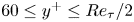 $60\le y^{+}\le Re_{\tau }/2$ where the time-averaged turbulence production and the time-averaged turbulence dissipation more or less balance, we have looked at time fluctuations of quantities averaged over $x,z$ wall planes but not over time. We have found that the time fluctuations of $C_\varepsilon ^{u_i,x_j}(t)$ (for $i=2$ and $j=1$, $i=2$ and $j=3$, and $i=j=3$) and $Re_{\varLambda }(t)$ are strongly anti-correlated at all wall distances considered. In fact, our low- and high-pass filtering operations have revealed that this anti-correlation is strong for both low and high frequencies, but for different reasons. For the low frequencies, the link between the anti-correlated fluctuations is the turbulent kinetic energy, whereas for the high frequencies, the fluctuations of both $K$ and $\varepsilon$ are important. In the case of $C_\varepsilon ^{w,z}(t)$, it has been possible to determine the cross-over frequency $f_c^*$ between these two behaviours, and we have found $f_c^{*}\sim u_{\tau }/y$ for $Re_{\tau } = 950$, but $f_c^* \sim u_{\tau }/\delta$ for $Re_{\tau }=2000$. This $f_c^*$ difference between these two Reynolds numbers appears to reflect the fact that whereas very large scale motions are present in the $Re_{\tau }=2000$ flow, they do not show similar signs of presence in the $Re_{\tau }=950$ flow. Irrespectively, though, the non-equilibrium dissipation scaling persists in both cases, suggesting that it is not affected by the structure of the flow but has a general validity that may prove useful in the future for better dynamical models for dissipation.
Acknowledgements
This work was supported by the European Community, the French Ministry for Higher Education and Research, and the Hauts de France Regional Council in connection with CNRS Research Foundation on Ground Transport and Mobility as part of the ELSAT2020 project. This work was granted access to the HPC resources of IDRIS under the allocation 2021-021741 made by GENCI (Grand Equipement National de Calcul Intensif). We are also grateful to M. Lee, R.D. Moser, A. Lozano-Durán and J. Jiménez for making their datasets available.
Funding
This work was supported by JCV's Chair of Excellence CoPreFlo funded by I-SITE-ULNE (grant no. R-TALENT-19-001-VASSILICOS), MEL (grant no. CONVENTION_219_ESR_06) and Region Hauts de France (grant no. 20003862).
Declaration of interests
The authors report no conflict of interest.
Appendix
In figure 14, we looked at the zero time lag correlation between filtered signals as a function of the cutoff frequency. The choice of constraining  ${\rm \Delta} t^+=0$ is motivated by observing figures 10 and 12, where we see the maximum absolute value of the correlation happening predominately at ${\rm \Delta} t^+=0$. To support this choice, we plot in figure 16 the location of the maximum absolute value correlation between the filtered signals for different wall-normal locations as a function of $f_c$. For the high-pass filtered signals, it is evident that the maximum absolute value correlation happens at zero time lag for $Re_\tau =950$ and all $C_\varepsilon ^{u_i,x_j}$ (figures 16b,f,j), and similarly for $Re_\tau =2000$ (figures 16d,h,l) except some particular $f_c$ and wall-normal locations, without, however, indicating a persistent behaviour, and perhaps as a result of the low time resolution. The low-pass correlations shown in figures 16(a,e,i) for $Re_\tau =950$, and figures 16(c,g,k) for $Re_\tau =2000$, support the argument that maximum anti-correlation happens at zero time lag, except for $Re_\tau =2000$ and $C_\varepsilon ^{w,z<}$, where we see that for increasing wall-normal locations, ${\rm \Delta} t^+$ increases as well, without, however, moving too far away from $0$, where significant values of anti-correlation also exist.

Figure 16. Plots of the time lag where the maximum of the absolute value of the two-time correlation occurs for low- and high-pass filtered signals of  $C_\varepsilon ^{u_i,x_j}$ and $Re_\varLambda$ against cutoff frequency $f_c$ premultiplied with $\delta /U_c$: (a,b,e,f,i,j) $Re_\tau =950$, (c,d,g,h,k,l) $Re_\tau =2000$. Plots show: (a–d) $C_\varepsilon ^{v,x}$, (e–h) $C_\varepsilon ^{v,z}$, (i–l) $C_\varepsilon ^{w,z}$. Finally, (a,c,e,g,i,k) show the maximum absolute value correlations of the low-pass filtered signals, while (b,d,f,h,j,l) show the high-pass ones. Different colours represent different wall-normal distances (15 in total).


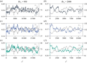


 Open access