


Introduction
Wherever it has been possible to observe the sole of a temperate glacier beneath a substantial thickness of ice, it has been found that the glacier ice contains considerable quantities of rock debris in the several centimetres immediately above its contact with the bed (Reference LewisLewis, 1960; Reference Kamb and LaChapelleKamb and La Chapelle, 1964; Reference PetersonPeterson, 1970; Reference Vivian and BocquetVivian and Bocquet, 1973; Reference Boulton, Wright and MoseleyBoulton, 1975). This debris is presumably derived from erosion of the bed and occurs in concentrations which are generally not more than about 30–40% by volume. The debris-studded glacier sole is an important erosive agent. Individual particles abrade the bed and cut striae at their points of contact, they are themselves comminuted, and are retarded relative to the moving glacier, presumably because of drag at the particle–bed contact (Reference Boulton, Wright and MoseleyBoulton, 1975). If the tractive force exerted by the moving ice is less than the total potential drag, then particles will not move over the bed and deposition of lodgement till will be initialed. This argument is supported by field observation.
If the frictional drag between debris particles and the glacier bed is large, and measurements of subglacial abrasion rates suggest that it must be, and if the particle concentration is high, then the presence of basal debris must be an important determinant of glacier sliding velocity. Ice must not only move over the relatively smooth, fixed obstacles on the rock bed of a glacier, but it must also move around the much “rougher” mobile obstructions to flow presented by debris particles. Thus, sliding of a glacier over its bed, the processes of erosion and deposition upon that bed, and the rates of these processes should be considered as interrelated problems.
The experiments described in this paper were undertaken in order to establish, by direct measurement of the basal shear stress, whether the basal-debris load could contribute a significant part of the drag force at the base of a glacier. The tests were conducted in summer 1973 and spring 1975 beneath the Glacier d’Argentière in the French Alps, where an extensive series of tunnels, constructed for hydro-electric purposes by Emosson S.A., pierce subglacial bedrock and allow access to the glacier–bed contact beneath 100 m of ice (Figs 1 and 2).

Fig. 1.
-
a. Map of the lower part of the Glacier d’Argentière. Contour heights in metres above sea-level. X–Y shows the location of the section in b.
-
b. Section along line X-Y, and the location of the cavity from which measurements were made.
-
c. Section along a flow line through the experimental area.

Fig. 2.
-
a. Plan of the vicinity of contact area B (Fig. 1c). The area of contact between the rock table and the glacier sole is stippled. In the rest of the area the glacier sole is underlain by a cavity. Flow lines on the glacier sole are shown in heavy lines. The location of a transducer in 1973 and 1975 is shown by T.
-
b. Section along c–d (Fig. 2a) showing the fold generated by deceleration produced by the drag offered by contact area B to glacier flow.
-
c. Section along a–b (Fig. 2c) showing the fold produced by “streaming” around contact area b.
Apparatus
The forces exerted by the ice on a small area of the bed were measured using transducers set into holes drilled in the bedrock. The upper load-measuring surfaces lay flush with the surface of the bed (Fig. 3). The transducers, developed in the Department of Engineering, University of Cambridge (Reference Arthur and RoscoeArthur and Roscoe, 1961), are manufactured by Robertson Research International of Llandudno, North Wales. Figure 4 shows the arrangement of foil-type strain gauges within the transducer. Gauges 1 to 4 are attached to the “N1” webs, gauges 9 to 12 to the “N2” webs and gauges 17 to 24 to the “S” webs. In the experiment the transducer was oriented with the “S” webs horizontal and parallel to the basal flow lines. A force applied to the rock platen which is bonded to the top surface of the transducer deforms the webs which connect it to the rigidly-held base of the transducer and alters the resistance of the strain gauges. A d.c. voltage applied to the three bridges produces output voltages N 1, N 2, and S. There is a small gap between the outer stainless-steel casing of the transducer and the rock platen. This is sealed with a flexible rubber seal designed to accommodate the small (<0.3 mm) movements of the platen produced by deformation of the webs. An inert silicone fluid prevents corrosion of the strain gauges. The thermal conductivities of the silicone fluid and the stainless steel are 20 × 10-4 J cm-1 s-1 deg-1 and 24 × 10-2 J cm-1 s-1 deg-1, respectively. The effective thermal conductivity of the transducer is of the same order as the thermal conductivity of the rock that it replaces (≈20 × 10-3 J cm-1 s-1 deg-1).

Fig. 3. a. Transducer set into bedrock near point A (Fig. 1c). Ice movement from left to right. A natural cavity occurs to the right. Note the thin debris-rich basal ice and the relatively clean ice above. b. Transducer on area B. The plate to the right is the transducer, the others measure abrasion. Ice movement from right to left. A thin, rapidly worn-off skim of cement rests on bedrock.

Fig. 4. The arrangement of strain gauges within the transducer.
The transducer was mechanically overloaded by 50% several times before it was calibrated. When the force was removed the circuits returned to their original zero without any significant time lag. The transducers were calibrated at 0°C using an input voltage of V ’ = 3 V. During our subglacial experiments, the input voltage V was passed through a voltage regulator and was held to within 0.5% of 3 V. With such a small variation in input voltage, the relationship between the input and output voltage for each gauge may be taken to be linear. Thus, for a given set of forces applied to the platen, the measured output voltages .N 1, N 2, and S, for input voltage V are related to the equivalent voltages N’ 1, N’ 2, and S’, for the input voltage V’ used for calculation by the equation

Let the set of forces on the platen which can produce deformation of the webs be equivalent to a single normal force P acting at a distance e from the centre of the platen in the direction of flow, and a shear force Q acting in the direction of flow. Then, the calibration curves for each transducer have the form

The values of the coefficients of the matrix A for the two transducers used in our experiments are given in Table I.
Table 1. Coefficient values for the matrix A for the transducers used in the experiments

During the experiments the voltages N 1, N 2, S, and V were measured and recorded by an MBM Minilogger with a digital voltmeter to a precision of ± 1 µV. Random errors in the measurements were not greater than ±5 µV except when the apparatus was first switched on. Since the input voltage V was monitored, errors arising from drift in the power supply were minimal (≤1 µV). Before calibration, the transducers were subjected to a mechanical and thermal ageing process so that all the errors arising from changes in the values of Aij with time, non-linear calibration curves, and hysteresis effects did not account for more than ± 10 µV. The combination of self-temperature-compensating strain gauges and the particular bridge-circuit design made the transducer extremely insensitive to temperature variations. Re-calibration of the transducer after the 1975 experiments failed to reveal any significant drift from the calibration recorded before the experiment.
Location of the experiment
The general location of the site (Fig. 1) has also been described by Reference Vivian and BocquetVivian and Bocquet (1973), Reference Souchez, Souchez, Lorrain and LemmensSouchez and others (1973), and Reference VivianVivian (1976). A natural cavity on the down-glacier side of a bedrock hummock allows easy access to the ice–rock interface (Figs 1c and 2a). The glacier sole first loses contact with the bed at point a and comes into contact again at b, a small area of rock with a gently sloping planar surface, smoothed and striated by glacial abrasion. Large cavities occur on the down-glacier side and the flanks of b. In this area the glacier thickness is about 100 m and its surface slope about 12° to the horizontal, giving an average basal shear stress of about 1.9 bar.
Observations show that the shape and extent of the cavity vary with the sliding velocity of the glacier. In plan (Fig. 2a), the ice flows past the bedrock hummock in a curved path. Fold structures and fractures in the basal ice show it to be in compression on the up-stream side and in tension on the down-stream side of the bedrock hummock. There is no resultant stress across the ice–air interface, and thus (deviatoric) tensile stress in the ice plus the hydrostatic pressure (about 10 bar for 100 m of ice) is equal to the atmospheric pressure in the cavity. On the up-stream side of the obstacle, where the ice must follow the contour of the rock, the rate of deformation normal to the ice-rock interface, and hence the compressive stress, must increase with increasing basal sliding velocity. On the down-stream side however, the tensile stress and rate of deformation normal to the ice–rock interface remain constant and thus the cavity becomes larger with increasing basal sliding velocity. Reference Vivian and BocquetVivian and Bocquet (1973) have confirmed that this is so.
On two occasions, in autumn 1973 and in spring 1975, we excavated the basal ice above surface b (1973 and 1975) and surface a (1973 only) and fitted stress transducers into holes in the bedrock (Fig. 1c). Relatively long data runs were obtained from the transducers fitted into surface b, but only a very short record was obtained from area a in 1973 before the transducer was mechanically overloaded. Polished rock platens of known thickness and surface roughness made up the load-bearing surfaces. In 1973 the platen was granite, in 1975 it was basalt. Quick-setting cement was used to fill the gaps between the transducer and the rock. A screened cable led from the base of the transducer through the bedrock to a terminal box in the cavity. The terminal box was connected by ten metres of screened cable to the power supply and a data logging system in a heated subglacial laboratory nearby.
The velocity of the glacier sole is measured some two metres to the south of the contact area b by the Vivian “cavitometer” (Reference Vivian and BocquetVivian, 1973, p. 446). This is a tyred bicycle wheel, 40 cm in diameter, held in contact with the glacier sole by a cantilevered arm. The wheel rotates according to the movement of the glacier sole. The rotation is measured using a continuously recording potentiometer. Unfortunately it is only possible to determine velocities averaged over a period of an hour. Measurements by Reference Vivian and BocquetVivian and Bocquet (1973) suggest that velocities within the vicinity of the cavitometer lie within 20% of the recorded values. The error in the recorded velocities is of the order of 0.5–0.75 cm h-1, and our independent measurements in April 1975 lie within this range of error (Fig. 5a).

Fig. 5. Results from an experiment on contact area b (Fig. 1c) in 1975.
-
a. Measurements of the velocity of the glacier sole adjacent to contact area b, and error bars.
-
b. Normal pressure.
-
c. Shear stress.
-
d. Eccentricity.
-
e. Structure of the basal ice which moved over the transducer during the experiment. The horizontal scale is a time scale and represents a distance scale adjusted to time using a. Measurements of volume concentrations of englacial debris were on spot samples of no more than 5 cm3. There are numerous thin laminae in this thin basal zone in which the debris concentration is less than 1%.
Structure of the basal ice
In the subglacial cavity in which the experiments were undertaken, and in other localities beneath the Glacier d’Argentière where the glacier sole could be inspected, it was found that the basal part of the glacier ice frequently contained high concentrations (up to 43% by volume) of rock debris. In general, it is found that this basal debris-rich ice does not extend more than a few centimetres above the glacier sole (although discrete debris-rich bands may sometimes occur up to one or two metres above the sole) and that this is overlain by clean ice. A similar observation has been made beneath several temperate glaciers (Reference LewisLewis, 1960; Reference Kamb and LaChapelleKamb and La Chapelle, 1964; Reference PetersonPeterson, 1970; Reference BoultonBoulton, 1975).
Figure 5e shows the debris distribution in basal ice which moved over the contact stress transducer during the measurement period in 1975. The basal debris-rich layer has an average thickness of 4 cm and a well-defined structure. The bottom millimetre or so of the layer is composed predominantly of silt-size debris which, we suggest, is generated by abrasion between the larger particles which penetrate through the glacier sole, and the rock bed of the glacier. These particles also striated the transducer platen (Fig. 6) and we presume from this evidence that they make “real” contact with the glacial bed. Large clasts, such as those shown in Figure 5e can be clearly seen to leave a silty trail in the basal ice, and also appear to plough up silt before them. Such ploughed-up masses of silt beneath and in front of large clasts which scratch the glacier bed have been also noted by Reference Boulton, Wright and MoseleyBoulton (1975) from beneath Breiðtamerkurjökull in Iceland. The basal layer of sill contrasts strikingly with the overlying debris, which has the wider range of grain sizes and the poor sorting typical of glacial till.

Fig. 6. Transducer used during the experiments from 4–9 September 1973. The rock platen on its upper surface is made of local granite and reached its striated state in about 18 d. It was originally cut by rock saw. The experiments were undertaken between days 12 and 17.
The debris particles form well-defined bands within the basal ice, which is itself more bubbly than the overlying clean ice.
The larger debris particles in contact with the glacier bed seem to form well-defined clusters, and the tendency for debris particles which are entirely suspended within the basal ice to form folds over these particles (Fig. 5e) suggests that the larger particles are retarded relative to the ice around them. From this we can infer that the drag between debris particles and the glacier bed is greater than between the adjacent ice and the glacier bed. Other signs of retardation are the cavities which frequently occur on the down-glacicr sides of large particles. Figure 7 shows such a particle with a cavity on its down-glacier side. The position and shape of the cavity reflect the shape of the spheroidal boulder behind which it occurs. Regelation ice spicules form in the cavity, attached either to the boulder or to the ice walls of the cavity, and are pulled out into a long stripe of clear regelation ice in the lee of the boulder as a result of ice flow relative to the moving boulder.

Fig. 7. Boulder (≈ 20 cm diameter) protruding from the glacier sole. Its base was originally flush with the glacier when this was in contact with bedrock, but frictional retardation of the boulder against bedrock, built up locally high hydrostatic pressures around it so that when the glacier sole lost contact with the bed the boulder began to be ejected from the ice. A small cavity coated with relatively clear regelation ice spicules occurs in the lee of the boulder, and where this cavity closes, the spicules are forced together to give a stripe of clear ice. The base of the boulder is heavily coated with rock flour produced by abrasion at the boulder–bed interface. Movement from top to bottom of the photograph.
Excavations have revealed that folding occurs in the basal ice at the point at which the glacier sole comes into contact with area b (Fig. 2a and b). The longitudinal velocity of the debris-rich ice in the glacier sole is reduced relative to the ice above and a well-defined fold is generated. As can be seen in Figure 2a, there is a strong lateral flow component of basal ice around the flank of contact area b, and the fold structure generated by compression against its up-glacier extremity appears to be accentuated as it flows around its flank. Thus, a transverse section at the edge of area b (Fig. 2c) shows the same type of fold structure, but oriented at right angles to the first structure. Because of this mode of flow, much of the debris-rich basal ice is diverted to flow around the margins of the contact area, and the ice which flows over the transducer is thus relatively depleted in debris. At times when the pressure measured by the transducer increases, it is found that the quantity of basal debris-rich ice forced to flow around the flanks of the bedrock knob is increased, and that the flux of debris over the transducer is therefore reduced. It has been suggested (Reference Boulton, Wright and MoseleyBoulton, 1975) that this debris “streaming” process is an important process beneath glaciers, resulting in the segregation of basal debris into longitudinal bands which also helps to produce differential erosion of the glacier bed.
Experimental results and observations
Results were obtained from transducers on contact area b (Fig. 2a) during three periods 4–8 September 1973, 4–5 October 1973 (17.00–15.00h), and 16–18 April 1975 (16.30–14.00 h). During the first two periods the data are incomplete, partly because of electrical faults and disruptions of the power supply during thunderstorms, and partly because of mechanical overloading of the transducers by large boulders within the basal ice. However, during two short periods, 10.30–10.35 h on 5 September 1973, and 14.30–22.30 h on 8 September 1973 all three voltages, N 1,N 2, and S were recorded. During a third period, from 17.00 h on 4 October to 15.00 h on 5 October 1973, records of N 1, and N 2 were continuous, although for much of the time the third circuit (S) was overloaded. The few S values obtained were, however, similar to those obtained earlier in September 1973 and are therefore regarded as reliable. The period from 16–18 April 1975 was trouble-free.
Figures 8, 9, and 10 show the voltages recorded by the three independent circuits corrected for changes in the bridge voltage during the three measurement periods. It is evident that for most of the time the behaviour of the circuits is linked. This indicates that the variations in voltage arise because of an external event common to all circuits (change in stress on the platen) rather than noise or the accumulation of static electricity, which would be different for each circuit.

Fig. 8. Voltages in circuits N1, N2, and S from 18.00 h on 4 September to 24.00 h on 8 September 1973.

Fig. 9. Voltages in circuits N1 and N2 on 4 and 5 October 1973.
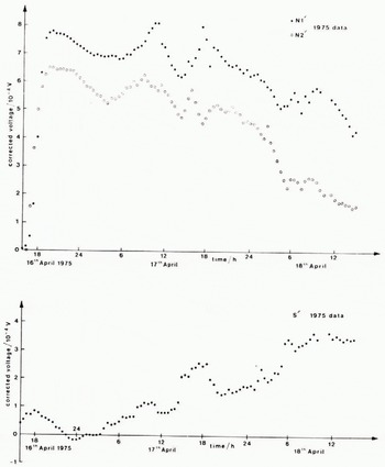
Fig. 10. Voltages in circuits N1, N2, and S from 16 to 18 April 1975.
Although the N1 circuit became overloaded on 5 September, its behaviour during the period 4–5 October shows that the web and strain gauge had not been damaged. Thus, we may accept values of N 1 measured during September. figure 11 shows the normal pressure, shear stress, and eccentricity for the period 14.30–16.00 h on 8 September 1973. The eccentricity can only be greater than half the width of the platen (≈15 mm) if there is a tensile stress on the up-stream half of the transducer. Thus, it is not likely that the values measured from 14.30 to 14.44 h are correct. Since these were the first measurements made after a long period of N1 circuit overloading, it was probably still reading high. This means that the calculated normal pressure and eccentricity would be too high and the shear stress too low. In the period 14.44 to 15.12 h, the electrical connections were checked and, for a short time afterwards, N 1 was much lower. In the period 15.12–15.58 h the eccentricity oscillates about zero and is never more than ±15 mm. We think these results are accurate. From 15.30 to 22.30 h the eccentricity is always positive and sometimes greater than 15 mm, though never more than 25 mm. It may well be that circuit N1 is again reading too high.
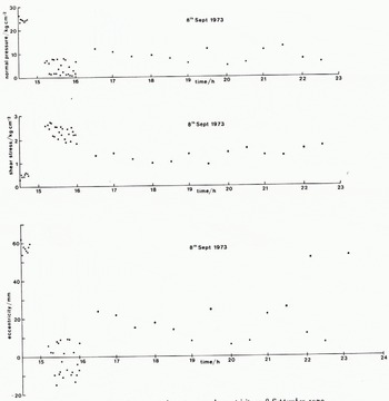
Fig. 11. Normal pressure, shear stress, and eccentricity on 8 September 1973.
The more continuous 1975 data are more useful for interpreting the detailed small-scale relationships which appear to exist between measured values of normal pressure, shear stress, and eccentricity. The detailed distribution of debris in the basal ice which passed over the transducer during the 1975 experiments was determined from observations made on the basal ice exposed in the roof of the cavity on the down-giacier side of contact area b, and on samples of this ice which were collected and brought back to the laboratory for study. Figure 5a–e shows the sliding velocity, normal pressure, shear stress, eccentricity, and debris distribution for the April 1975 period. The horizontal scale has been changed from a length scale to a time scale with the aid of the velocity measurements in order to show the nature of the basal ice over the centre of the transducer at any moment during the experiment.
The hourly-mean velocity varies between 1 and 3.5 cm h-1 with a mean value of 1.9 cm h-1. These values are similar to those obtained by Vivian and Bocquet in October 1972 using the same cavitometer (Reference Vivian and BocquetVivian and Bocquet, 1973). There is no overall change in velocity corresponding to the decline in pressure and increase in shear stress, and no clear correlation between fluctuations in velocity and shear stress. It appears, however, that the major fluctuations in normal pressure, shear stress, and eccentricity are related to the passage over the transducer of relatively large debris particles or groups of particles.
There are several contrasts between the data obtained in 1973 and 1975. In 1975 there was a long-term trend of decreasing pressure and increasing shear. In 1973 there was no such trend. We show the voltages for both periods so that short-term fluctuations can be compared. In 1973 the debris moving over the platen had a finer grain than that in 1975 (although no detailed measurements were made in 1973), and the 1973 data (Fig. 8) show smaller peaks associated with clasts moving over the transducer than do the 1975 data (Fig. 10).
Interpretation of experimental data
After both experiments, in 1973 and 1975, it was possible to remove the transducers and examine the rock platens. Figure 6 shows the platen used in 1973. The rock is granite, composed primarily of crystals of quartz and felspar up to ten millimetres in diameter. The platen was originally ground to a smooth surface by a rock saw and was roughened during the course of the experiments. The theory of Nye (Reference Nye1969, Reference Nye1970) predicts the average shear stress <τ> exerted on a surface of given roughness by clean ice moving over it at a given velocity. He gives

where Xav = 0.04 m is the length of the platen in the direction of ice motion, U ≈ 5.6 × 10⁻⁶ m s-1 is the basal sliding velocity, η ≈ 3 × 10¹² Pa s is the viscosity of the ice treated as a Newtonian fluid, K* ≈ 10 m-1 is the critical spatial angular frequency and a = 4r2/0. 148 where r is the surface roughness. The measured roughness of the platen at the end of the 1973 experiments was r = 0.004±0.001, and at the end of the 1975 experiments r = 0.002±0.001, in the range Xav = (3—17) x 10 -3 m. (The running-mean method for averaging was used.) Thus,

The shear stresses measured were an order of magnitude higher than these values. We suggest that this reflects the presence of debris particles in the basal ice, a factor which is omitted from the sliding theory.
An analysis was undertaken of 257 measurements of shear stress and pressure at ten-minute intervals from the 1975 results. Because of the high effective viscosity of ice we do not expect to find very-high-frequency events. The data available at smaller, one-minute sampling intervals fail to reveal any high-frequency structure not resolved by the larger sampling interval. The long-term trend is removed using simple linear-regression equations against time T (Fig. 12). The resulting series shown in Figure 13 appear to show three principal pressure and shear events; in pressure, a peak at 60, a plateau at about 125, and a small hump at 215; in shear, a decline from 0, a peak at 120, and a plateau at about 190–200.

Fig. 12. Overall linear trends of the relationships between normal pressure and shear stress during the 1973 and 1975 experiments.
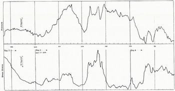
Fig. 13. Normal-pressure and shear-stress data for the experiments on 16 to 18 April 1975.
There are thus three principal features of the data series which require explanation; a long-term trend of falling pressure and increasing shear (Fig. 12); a low-frequency event, in which two large waves of pressure and shear of similar form (Fig. 13) are offset by 400–600 min; and a high-frequency variation associated with the passage of individual stones over the transducer. This high-frequency variation can be shown to be associated with stone movement from the evidence of a continuous plot of pressure against shear (Fig. 14). We refer to the high-frequency events as small-scale effects, and to the lower-frequency events and the long-term trend as medium-scale effects.

Fig. 14. Continuous plot of shear stress against normal pressure. The increase of pressure at constant shear represents initial movement of ice over the transducer after the latter’s emplacement. The subsequent loops can be clearly correlated with the passage of stones over the transducer (Fig. 5e).
Small-scale effects—the passage of individual particles over the transducer
Comparison of Figures 5e and 13 clearly shows that most of the small-scale effects on the transducer records are related to the passage of individual particles or groups of particles over the transducer; both pressure and shear rise as this occurs. This is also seen in the continuous plot of pressure versus shear (Fig. 14) where individual loops and groups of loops can be directly correlated with the passage of stones or groups of stones over the transducer. Such a plot also shows that pressure and shear do not rise and fall in unison as stones move over the transducer, although the loop patterns are complex, resulting perhaps from complex interactions between particles. An example of the detailed pattern of eccentricity shear and pressure as stones pass over the transducer is given in Figure 15. This shows the record for the passage of a stone 5 cm in diameter over the transducer, this transition took from 06.00 to 12.00 h on 17 April 1975. The pattern of eccentricity, pressure, and shear is, in broad outline, typical of the passage of stones over the transducer, although the detailed pattern may vary from event to event. The minimum eccentricity appears to coincide with a stone position in which the contact point of the stone has moved a short distance onto the transducer, and the maximum eccentricity coincides with a position in which the contact point lies over the down- glacier extremity of the transducer. This gives a mean stone velocity of 1.5 cm h-1 between 09.00 and 11.00 h, a value which lies within the error limits for velocity measured by the cavitometer. Thus, although the stone velocity is close to the ice velocity, we cannot say whether the two are the same or whether the stone is retarded relative to the ice. The large instrumental errors in velocity measurement do not enable us to compare stone velocity and ice velocity at any time.

Fig. 15. Record of normal pressure, shear stress, and eccentricity during passage of a stone over the transducer between 06.00 and 12.00 h on 17 April 1975.
Figure 16 shows a simplified example to explain how we believe the features shown in Figure 15 arise. We know that the presence of a stone produces an increase in the normal pressure on the bed in its vicinity. We discuss why this should be so later on. Let the overburden pressure be, for example, 16 bar and the amplitude of the normal pressure variation, averaged over 3 cm transverse to the direction of flow, be 8 bar. The pressure is transmitted to the bed through, first, a solid contact with a coefficient of friction μ = 0.4 extending for, say, 0.25 cm in the flow direction, and then through the ice which is assumed to exert no friction on the transducer. The records that would be produced by a transducer with a 3X3 cm2 platen as this stone moved over it at a steady 1 cm h-1 have all the features which were observed in the experimental records. Normal pressure begins to rise before shear stress because the ice around the stone transmits pressure but has a very low friction coefficient. For the same reason, shear stress drops to zero before normal pressure. The eccentricity falls then rises as the stone moves across the platen.
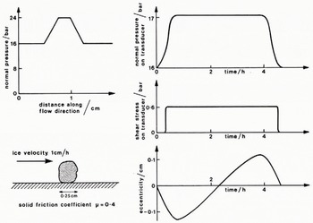
Fig. 16. Schematic diagram showing general changes in normal pressure, shear stress, and eccentricity measured by the transducer during the passage of a stone over it. Normal pressure rises before and falls after shear stress as the ice around the stone transmits pressure but has a lower frictional coefficient than the stone. Movement of the stone over the transducer produces a phase of negative pressure eccentricity followed by positive eccentricity. The velocity of the stone can be estimated from this latter effect.
We believe that there are several processes by which a stone moving over a glacier bed might exert a normal pressure greater than the overburden pressure and over an area greater than the area of contact between stone and bed. These are illustrated in Figure 17a–e. Figure 17a shows what might be called a “hydrostatic” model for this interaction. If water is free to drain from the basal water layer its pressure p = pw may fall below the overburden pressure p 0. The normal pressure p (x) exerted by the stone through solid–solid contact is then greater than p 0 so that p (x) dx = p 0 dx and hydrostatic equilibrium is maintained. Since pw < p o the ice will flow towards the bed between the stones. However, this process may be counteracted by geothermal and frictional melting which will tend to increase the size of the water layer.
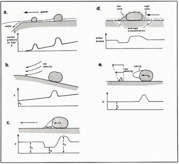
Fig. 17a–e. Processes leading to fluctuations of pressure and shear in the vicinity of stones in traction over the glacier bed. c and d are probably the most important causes of the fluctuations measured during our experiments.
The drainage path from the position where the measurements were made to an open cavity was very short (≈ 0.6 m), and it seems likely that such conditions of easy drainage into open cavities which exist beneath rapidly flowing glaciers such as the Glacier d’Argentiére will maintain the condition where pw < p 0. A similar argument to this has been presented by Reference LliboutryLliboutry (1968) and Reference WeertmanWeertman (1972) who suggest that obstacles on the glacier bed will pierce the basal water layer so as to reduce pw .
Figure 17b and c shows cases in which normal pressure may increase because ice moving around the stone exerts a net force normal to the bed. In Figure 17b the ice is moving over a bedrock hump and there is a vertical component of velocity. The stone cannot move with the ice and again a net downward force on the stone is transmitted to the bed as an increased normal pressure. In Figure 17c, friction between the stone and the bed causes retardation of the stone relative to the moving ice, and causes ice to flow past it in such a way as to increase the pressure in its vicinity.
We explain the fluctuations in shear stress as due to variations in the debris content of basal ice in the vicinity of a stone, and expect the highest shear stresses to occur at the contact between stones and the bed. Figure 17d shows typical variations in debris content in the vicinity of a stone and the fluctuations in shear stress which we would expect to find.
Many of the larger stones which we have observed show cavities in their lee (Fig. 7) which may allow drainage of the basal water layer. Suppose that a stone has dimensions α and a down-stream cavity (Fig. 17d–e). Ice moves around the stone in such a way that the normal pressure at the ice–cavity interface pa is less than the overburden pressure p0 and the normal pressure on the up-stream face of the stone is greater than p 0. Suppose, for the sake of an order-of-magnitude argument, that the normal pressure variation is symmetric. Then, the pressure difference across the stone is ≈2(p 0—pa ). The normal force exerted by the stone on the bed through rock–rock contacts is ≈ (p 0—pw ) α2 + (ρr—ρi) gα3 where ρr and ρi are the densities of rock and ice. Thus, the force on the stone in the down-slream direction 2(po —pw ) α2, is opposed by a frictional force μ{(po —pw ) α2+{ρr — ρi) α3}. For a steady-state situation
and, therefore,
With g = 9.81 m s-2, ρr—ρi ≈ 2 × 10³ kg m-3, μ ≈ 0.5, p w = p a = o, and p 0 = (1–10) bar, we have α ≥ 10–100 m.
For stones of normal size, the force exerted by the ice is much greater than the retarding friction so that the relative velocity between ice and stone cannot be maintained. Thus, this process can only produce an increase in normal pressure on the bed for a limited time.
On the small scale, the process which produces shear stress on the glacier bed is solid friction between the bed and stones passing over it. However, this does not mean that a simple solid-friction law can be used as the lower boundary condition for glacier-flow studies; medium-scale processes must be taken into account.
Medium-scale effects
Our analysis of the 1975 data shows a long-term trend in which pressure and shear are inversely related (Fig. 12). In the 1973 data we see a similar inverse relationship between pressure and shear stress (Fig. 12). The reality of the trend of decreasing pressure in 1975 is reflected by the rise of the cavity roof measured by the cavitometer. There is no similar long-term trend with time in 1973. This difference, the absence of a trend in eccentricity, and the return of voltages to their original unloaded values after the transducer was extracted suggest that any temporal trends are not implantation effects. Although both the 1973 and 1975 data sets show an inverse relationship between pressure and shear stress, the effects appear in different parts of the graph. We believe that this relationship can be explained by an analysis of the flow pattern of ice over and around the contact area on which the measurements were made (Fig. 2). Because of the streaming of ice around this contact area, much of the debris-rich basal ice is diverted around the margins of the contact area and the ice that flows over the transducer is thus relatively depleted of debris. When the normal pressure increases, the proportion of basal debris-rich ice forced to flow around the flanks of the bedrock knob also increases. Thus the flux of debris over the transducer is reduced. The maximum value of the ratio μ(shear stress/normal pressure) is 0.44, which may be compared with the value for μ of 0.65 for solid friction between two granite surfaces. Although we believe that the local relationship between pressure and shear depends on a solid-friction mechanism, the variation in concentration of debris from place to place, which may be related to bed profile, means that a simple solid-frietion law for basal shear stress cannot be used in the analysis of glacier flow problems.
The discrete events of pressure and shear (Fig. 13) which are superimposed on the general trend of the 1975 data appear to show a rise in pressure followed by rise in shear after a lag time of 400–600 min. We suggest that this can be explained by a consideration of the detailed form of the bed immediately up-glacier of the transducer. Figure 2a shows a sketch plan of the area around the transducer. There is a well-defined step, about 3 cm deep, in the rock bed some 20 cm up-glacier of the transducer. It is aligned at right angles to the ice flow, but leads into a furrow which swings around until it runs parallel to the ice flow.
When ice flows against this step, the basal ice is diverted laterally into the furrow and thus does not flow over the transducer. As will be seen in Figure 5e, the highest volume concentration of debris occurs in the basal part of the ice, and this decreases upwards. Thus, the diversion of basal ice around the transducer reduces the debris concentration of ice flowing over the transducer (we therefore assume that we could have measured much larger shear forces had we placed the transducer elsewhere). Thus, if for some reason the local ice load on the bed increases (due to glacier thickening or reduction in velocity, or to changes in the pattern of ice flow), we expect that increased compression against the step would cause an increased diversion of ice into the lateral, unconfined position, and thus reduce the debris content in the basal ice which subsequently flows over the transducer. The increased pressure will be recorded immediately at the transducer, but the change in shear stress resulting from decrease in debris content will not be felt for the order of 400 to 600 min, which is the time laken for the ice to flow the 20 cm from the small step to the transducer.
Thus, if a glacier flows over a bedrock hummock around whose flanks cavities occur, an increase in ice overburden pressure, or a decrease in ice velocity will cause the glacier to press down lower over the hummock and reduce the volume of cavities. As it is the basal debris- rich ice which will be diverted to flow into these lower points of the bed, it is to be expected that the debris concentration will be reduced over high points of the bed and increased over low points of the bed. If no cavities exist, then the debris concentration at any one locality will not be expected to change in response to pressure or velocity changes, but we still expect contrasts between high points overlain by relatively thin basal debris layers, and low points into which flow has concentrated the basal debris into a thicker layer.
This “streaming effect” (Reference Boulton, Wright and MoseleyBoulton, 1975) can observed beneath many glaciers. Observations in the lee of a series of bedrock hummocks beneath Breiðamerkurjökull in Iceland show that over the tops of the hummocks the debris-bearing basal ice has a thickness of about ten centimetres, but in the troughs between the hummocks the debris-rich ice is up to one metre thick, and the foliation patterns in the ice clearly reflect diversion of debris-rich ice from the up-glacier flanks of hummocks into intervening trenches to form thick, dense accumulations, although the maximum volume concentration recorded is 55% (Boulton, in press).
Conclusions
The experimental data presented here show that:
-
(1) significant frictional forces are developed between particles of debris embedded in the basal ice of a glacier and the glacier bed,
-
(2) the coefficient of friction is dependent on the concentration of debris particles in the ice, and
-
(3) the concentration of debris commonly found in the basal part of glaciers is sufficiently high for a significant proportion of the drag at the glacier bed to be contributed by such mineral debris.
Acknowledgements
We are very grateful to Robert Vivian and Gerard Bocquet for making our experiments possible, and to Electricité de France, Electricité d’Emosson, and Pegaz et Pugeat for permission and assistance in working in the subglacial galleries at Argentière. Frank Grynkiewicz and Richard Hindmarsh helped with the field work, and Barbara Gray made useful comments on the statistical analyses. This work was financed by the Natural Environment Research Council (Grant GR3/2001).


