


1. Introduction
1.1. Motivation and scope
Spatial acceleration is encountered in a wide range of engineering applications such as turbomachinery, aerofoils and wind turbines in addition to natural processes such as atmospheric flows. Additionally, such flows contain interesting, incompletely understood phenomena that can have a significant impact on flow physics. Improving the understanding of these flows may also have an impact on emerging topics in the study of turbulence such as flow control and drag reduction. One of the most important phenomena of these flows is laminarisation, which has been observed in accelerating flows for more than 50 years. Unanswered questions remain including, for example, the so-called island of ignorance, which was used by Sreenivasan (Reference Sreenivasan1982) to describe the process by which a fully developed turbulent flow reverts to a more laminar-like state although there have been recent attempts to explain this (Bourassa & Thomas Reference Bourassa and Thomas2009; Piomelli & Yuan Reference Piomelli and Yuan2013). There are also open questions related to the process of retransition, where the flow returns to the turbulent state following laminarisation. It has been noted in a number of studies that the boundary layer is highly perturbed prior to retransition (Sreenivasan Reference Sreenivasan1982; Escudier et al. Reference Escudier, Abdel-Hameed, Johnson and Sutcliffe1998). As a result, the process of retransition differs from the processes often observed in natural transition or bypass transitions of relatively low free-stream turbulence (FST).
At the forefront of the research into temporally accelerating flows, some new perspectives have been proposed to explain the transient turbulent flow phenomena (He & Seddighi Reference He and Seddighi2013, Reference He and Seddighi2015; Mathur et al. Reference Mathur, Gorji, He, Seddighi, Vardy, O'Donoghue and Pokrajac2018). The transient development of such flows was characterised by the laminar-to-turbulent bypass transition of a new boundary layer which formed at the onset of acceleration. The purpose of this paper is to demonstrate that a spatially accelerating flow exhibits similar characteristics with a new boundary layer forming superimposed on the pre-existing turbulent flow in response to the flow acceleration. Initially, this new boundary layer does not significantly modify the characteristics of the flow. Only following the development of the new boundary layer downstream does a spontaneous transition occur, resembling that seen in bypass transition, bringing the flow to a new state commensurate to the increased flow rate. This study is based on direct numerical simulations (DNS) of a spatially accelerating flow using a novel methodology which applies a non-zero, increasingly negative streamwise velocity on the channel walls. The relative acceleration between the fluid and the wall permits an investigation of the effects of flow acceleration without some of the other intrinsic features of conventional (conventional in the sense of the acceleration being caused by the contraction of the flow resulting in velocity increases through mass continuity) spatially accelerating flows such as streamline contraction. While this does not capture all aspects of spatially accelerating flows, it enables a study of the response of turbulence to bulk flow acceleration alone, albeit under idealised conditions. In addition to the study of the nature of transition in this flow, the similarities and differences between the moving-wall flow and more conventional spatial accelerations are discussed.
In the remaining sections of the introduction we will first review the literature on spatially accelerating flows and summarize the prevailing understanding and theory on the turbulence behaviours in such flows in order to set the scene for the new development presented in this paper. This is followed by a review of the current research on bypass transition to facilitate the discussion on the proposed interpretation. Finally, recent developments in temporal acceleration are reviewed to form a base for a comparison between the moving-wall acceleration and temporally accelerating flows.
1.2. Studies of spatial acceleration
Launder (Reference Launder1964) was an early study to investigate the accelerating flow through a two-dimensional nozzle identifying some of the key features of such flows. It was found that in the second half of the nozzle there were rapid increases in the shape factor and a decrease in the skin friction coefficient consistent with a reversion towards the laminar state, a process labelled as ‘laminarisation’. The degree of acceleration is often defined in terms of the acceleration parameter,  $K=({\nu }/{U_\infty ^2})({{\rm d}U_\infty }/{{\rm d}\kern0.06em x})$. A number of authors have found similar values for the onset of laminarisation. Kline et al. (Reference Kline, Reynolds, Schraub and Runstadler1967) and Schraub & Kline (Reference Schraub and Kline1965) found that during severe acceleration there were reductions in near-wall bursting and at $K=3.7\times 10^{-6}$ bursting was found to have ceased. This broadly coincided with the condition at which Moretti & Kays (Reference Moretti and Kays1965) observed a reduction in heat transfer rate, consistent with a reversion to laminar.
Badri Narayanan & Ramjee (Reference Badri Narayanan and Ramjee1969) confirmed the behaviour of skin friction coefficient,  $C_f$ and the boundary layer shape factor observed in the previous studies and found that the streamwise normal Reynolds stress normalised with respect to the local free-stream velocity decayed exponentially. The wall-normal distribution of the streamwise Reynolds stress exhibited near similarity when normalised by its local maximum value and the wall-normal distance of the maximum. This implies that some characteristics of the structure of the turbulence are retained in the acceleration. Blackwelder & Kovasznay (Reference Blackwelder and Kovasznay1972) investigated the role of large eddy structures during laminarisation. It was found that the streamwise turbulence intensity decreased, although this was mostly the result of increasing free-stream velocity. The maximum of the streamwise Reynolds stress was found to move outward from the wall during the acceleration. The streamwise velocity autocorrelation, compared with an unaccelerated case, indicated that the structures had been elongated in the spanwise direction and to a smaller extent in the streamwise direction.
Narasimha & Sreenivasan (Reference Narasimha and Sreenivasan1973) was another important contribution to this subject. The study described the process of the laminarisation occurring in severe spatially accelerating flows into four stages: fully turbulent (I), the region after the onset of acceleration where the flow remains fully turbulent; reverse transitional (II), a region where the flow becomes increasingly laminar-like; quasi-laminar (III), where the statistics of the flow are essentially laminar; and retransition (IV), where the flow returns to the turbulent state, typically after the relaxation of the acceleration. It also noted that during the acceleration, the laminarisation was caused by the domination of the pressure forces over the Reynolds stresses, which remained ‘frozen’ during the acceleration. The turbulent flow structures were not necessarily destroyed during regions II and III but that they merely did not contribute significantly to the dynamics of the flow. A later study (Narasimha & Sreenivasan Reference Narasimha and Sreenivasan1979) referred to this relative phenomenon as ‘soft’ laminarisation. The 1973 study also developed a two-layer quasi-laminar model consisting of a laminar inner layer and an inviscid outer layer, which was found to predict the overall flow well, although there were significant departures in region II, corresponding to the island of ignorance referred to in the introduction. Dixit & Ramesh (Reference Dixit and Ramesh2010), with the aid of experiment, explained the unexpected success and limitations of the two-layer model in terms of the effect of the acceleration and the streamline contraction on a typical eddy in the form of a simplified hairpin-like vortex.
The review article of Sreenivasan (Reference Sreenivasan1982) summarised the progress in the understanding of spatially accelerating flows up until that point. Since then, there have been a number of consequential experimental studies of spatial acceleration. McEligot and co-workers used an innovative laterally converging duct to investigate spatial acceleration (Chambers, Murphy & McEligot Reference Chambers, Murphy and McEligot1983; Murphy, Chambers & McEligot Reference Murphy, Chambers and McEligot1983; McEligot & Eckelmann Reference McEligot and Eckelmann2006). Changes to the mean velocity profile were found, with an upward shift of the log law layer and a thicknening of the viscous sublayer, which had also been found in previous studies (Patel & Head Reference Patel and Head1968; Blackwelder & Kovasznay Reference Blackwelder and Kovasznay1972). The studies also noted that the characteristic most affected by the acceleration was bursting frequency. By studying the inner-scaled probability distributions of  $v'$ and $u'v'$, it was found that larger magnitude sweep and ejection events were more common in the accelerated flow. Escudier et al. (Reference Escudier, Abdel-Hameed, Johnson and Sutcliffe1998) found similar features to previous studies regarding the shape of the mean velocity and the turbulence intensity profiles. It was also one of the relatively few studies to examine retransition, noting that it was more complicated than typical laminar-to-turbulent transition due to the remaining turbulent structures of the laminarised flow. Fernholz and Warnack produced a pair of experimental studies (Fernholz & Warnack Reference Fernholz and Warnack1998; Warnack & Fernholz Reference Warnack and Fernholz1998) investigating turbulent boundary layers with constant and favourable pressure gradients. This study highlights the difference between the locally scaled and absolute changes in the normal Reynolds stresses, particularly the streamwise component. When inner scaled, the streamwise Reynolds stress was shown to decrease during the laminarisation, however, in absolute terms it exhibited downstream growth until the onset of retransition. It should be noted that some earlier studies found an absolute decay across all normal Reynolds stress (Sreenivasan Reference Sreenivasan1982). This discrepancy may be explained by the manner in which the results are presented, being displayed against streamfunction or at constant wall-normal distance. This is supported by the results of Piomelli & Yuan (Reference Piomelli and Yuan2013). The effect of the laminarisation on the energy spectra is also presented with the disappearance of the $k^{-5/3}$ law indicating the absence of an inertial subrange which had similarly been observed in Jones & Launder (Reference Jones and Launder1972), a study on sink flows. Bourassa & Thomas (Reference Bourassa and Thomas2009) among other analyses, conducted quadrant analysis and found that the sweep and ejection events compared with the local eddy turnover time were significantly reduced, although the remaining ejection events were strengthened. This was explained by the effect on the streaks of an increase in the spanwise vorticity and a reduction of the wall-normal vorticity, which are caused by the acceleration and the increasing spanwise separation of the streaks, respectively. This then results in the formation of fewer vortices which are stronger due to acceleration-induced stretching. Consequently, this led to uncharacteristically more violent events, which correlates with the findings from the previous studies (McEligot & Eckelmann Reference McEligot and Eckelmann2006; Bader et al. Reference Bader, Pschernig, Sanz, Woisetschläger, Heitmeir, Meile and Brenn2016).
There have also been significant numerical studies to investigate spatial acceleration. An early attempt was Spalart (Reference Spalart1986), which used DNS to investigate sink flows comparing results with an experimental study (Jones & Launder Reference Jones and Launder1972) with satisfactory agreement. The study noted that near-wall streaks were still present in all flows and that even at  $K=2.5\times 10^{-6}$ these structures had not been suppressed. Finnicum & Hanratty (Reference Finnicum and Hanratty1988) investigated favourable pressure gradient flows with an innovative computational model which considered just a small wall-normal extent of 40–70 wall units. The turbulent kinetic energy budgets indicated that despite the boundary layer being quasi-laminar, production remained although when inner scaled all terms still reduced. Piomelli and co-workers have conducted a series of computational studies on accelerating flows. Piomelli, Balaras & Pascarelli (Reference Piomelli, Balaras and Pascarelli2000) noted that during the acceleration, the streaks and coherent eddies were elongated. The former also contained fewer disturbances due to the relative decrease in the spanwise fluctuations compared with its streamwise counterpart. A further significant paper was Piomelli & Yuan (Reference Piomelli and Yuan2013), which found that the pressure strain (in wall units) reduced just prior to the onset of laminarisation and recovered with the onset of retransition indicating that energy redistribution contributes to the processes of laminarisation and retransition.
1.3. Bypass transition
Early research on transition tended to focus on natural transition via the generation and propagation of Tollmein–Schlichting waves, which cause three-dimensional secondary instabilities leading to turbulent spot generation and transition. These disturbances grow slowly on viscous time scales in an exponential manner. At high levels of FST ( $Tu>1\,\%$) disturbances in the boundary layer grow rapidly resulting in a much earlier breakdown to turbulence which bypasses the Tollmein–Schlichting wave mechanism. This is consequently known as bypass transition. The process of bypass transition is well described as a three-phase development (Jacobs & Durbin Reference Jacobs and Durbin2001): the buffeted laminar boundary layer, the intermittent region and the fully turbulent boundary layer. In the first region, disturbances from the free stream perturb the boundary layer where shear sheltering results in only the lower frequencies penetrating it, a process known as receptivity. These are amplified by the mean shear resulting in the formation of elongated streaks of alternating positive and negative streamwise velocity. These streaks develop downstream until in the second region, where secondary instabilities form on some of these streaks resulting in their breakdown into turbulent spots which grow until the entire wall is covered in turbulence. One of the pioneering studies of bypass transition was Klebanoff (Reference Klebanoff1971), which identified streaks in the early stages of bypass transition which have since been often referred to as Klebanoff (Reference Klebanoff1971) modes. Voke & Yang (Reference Voke and Yang1995) highlighted the importance of the free-stream disturbances in causing subcritical transition and noted that the onset of transition coincides with a significant increase in the pressure strain redistribution of energy from $u^\prime$ into $v^\prime$.
Research by Jacobs & Durbin (Reference Jacobs and Durbin2001) was based on the DNS of a spatially developing boundary layer with a synthetic inlet based on Orr–Sommerfeld modes. The study identified that streak breakdown often occurred on individual, slow-moving streaks termed ‘backward jets’. One potential mechanism is due to them being lifted-up from the near-wall region causing them to interact with high-frequency FST resulting in Kelvin–Helmholtz-type secondary instabilities leading to breakdown. It was found that backward jets lying above faster-moving positive jets are particularly unstable. The peak in the streamwise Reynolds stress is initially in the mid-boundary layer before settling closer to the wall downstream, assuming a profile consistent with the formation and development of Klebanoff modes. In an experimental study, Matsubara & Alfredsson (Reference Matsubara and Alfredsson2001) found that the streamwise disturbance energy increases proportionally to downstream distance and that the critical Reynolds number has an inverse square relationship with the FST intensity. The study also investigated the scales of near-wall streaky structures finding that as downstream distance increases the spanwise scale approaches the boundary layer thickness having initially been larger than it, although there is no dramatic change in the spanwise scale. Much of these observations are in-line with the theoretical studies on transient growth theory by Andersson, Berggren & Henningson (Reference Andersson, Berggren and Henningson1999) and Luchini (Reference Luchini2000), which suggested a linear receptivity mechanism where the optimal free-stream disturbances were quasi-streamwise vortices developing into streaks through the lift-up mechanism. Building on earlier work by several authors on transient and non-modal growth (Ellingsen & Palm Reference Ellingsen and Palm1975; Landahl Reference Landahl1980; Trefethen et al. Reference Trefethen, Trefethen, Reddy and Driscoll1993), the development of these optimal disturbances was found to be able to predict well the wall-normal profiles of  $u^\prime _{rms}$ from experiments (Westin et al. Reference Westin, Boiko, Klingmann, Kozlov and Alfredsson1994), although the spanwise scale variations described above could not be adequately predicted. A nonlinear receptivity mechanism, described in Berlin & Henningson (Reference Berlin and Henningson1999), was stated to be able to continuously force streaks inside the boundary layer and was found to resolve differences in spanwise scale between the experiment and theory. Fransson & Alfredsson (Reference Fransson and Alfredsson2003) found that the spanwise scale also depended on the length scales of the FST.
There have also been significant investigations into the secondary instabilities causing streak breakdown. Asai, Minagawa & Nishioka (Reference Asai, Minagawa and Nishioka2002) experimentally investigated the breakdown mechanisms of a single streak through acoustic excitement, identifying a varicose (spanwise symmetric) and a sinuous (spanwise antisymmetric) instability mode. The former was found to be a Kelvin–Helmholtz instability of the inflectional wall-normal velocity profile, whose growth rate reduces as a streak's spanwise scale increases. The latter mode was not strongly affected by streak width and, hence, could propagate farther downstream. Brandt, Schlatter & Henningson (Reference Brandt, Schlatter and Henningson2004), using DNS and a synthetic inlet, found that the streak breakdown discussed in Jacobs & Durbin (Reference Jacobs and Durbin2001) was of the varicose type being caused by the head of a high-speed streak reaching the tail of a low-speed streak, although breakdown could also be caused by ‘backward jets’ being lifted-up and interacting with the free stream consistent with observations of Jacobs & Durbin (Reference Jacobs and Durbin2001). The study also found that the sinuous breakdown was found to be caused by a higher-speed streak passing on one side of a low-speed streak causing an inflectional spanwise velocity profile. Streak collisions and interactions were further studied in Brandt & de Lange (Reference Brandt and de Lange2008). The study also found that higher FST intensities and larger integral length scales caused earlier transition. However, Fransson & Shahinfar (Reference Fransson and Shahinfar2020) found that the picture is more complex, and an increase in integral length scale only advances transition at low FST while at high FST transition is postponed. Hack & Zaki (Reference Hack and Zaki2014) carried out a stability analysis and found that low-speed streaks could break down through interactions with the FST or collisions with high-speed streaks, confirming the observations of Brandt et al. (Reference Brandt, Schlatter and Henningson2004). Nolan & Zaki (Reference Nolan and Zaki2013) found that the spot inception was related to streaks with large perturbing velocity amplitude exceeding 20 % of the free-stream velocity. Schlatter et al. (Reference Schlatter, Brandt, de Lange and Henningson2008) found that the sinuous mode caused breakdown more frequently than the varicose mode and that it resembles a wavepacket-like secondary instability, which grows as it disperses downstream. Eventually, the flow breaks down forming a turbulent spot. The nature of the turbulent spots which formed as a result of this breakdown was investigated in Marxen & Zaki (Reference Marxen and Zaki2019) using DNS and conditional averaging of the spots. They found that in the centre of the large spot the statistics were consistent with fully developed turbulence, while towards the edges this was not the case. The role of the streaky structures in the breakdown to turbulence has also been studied by Mandal, Venkatakrishnan & Dey (Reference Mandal, Venkatakrishnan and Dey2010) and Nolan, Walsh & McEligot (Reference Nolan, Walsh and McEligot2010) through proper orthogonal decomposition and quadrant analysis, respectively, the latter noting the growth in ejection (Q2) events related to the uplift of the negative streaks and subsequent interaction with higher velocity fluid resulting in breakdown. Wu & Moin (Reference Wu and Moin2009) investigated bypass transition using a novel approach with an intermittent patch of isotropic turbulence introduced at  $Re_\theta =80$. In contrast to many of the studies discussed above, they proposed that transition is caused by hairpin vortices resulting from the nonlinear development of $\varLambda$ vortices with the streaks being a symptom of this development. Wu et al. (Reference Wu, Moin, Wallace, Skarda, Lozano-durán and Hickey2017) indicated that streak breakdown facilitates the growth of turbulent spots rather than causes their inception.
Nagarajan, Lele & Ferziger (Reference Nagarajan, Lele and Ferziger2007) performed numerical simulations of the flow over a flat plate with a super-elliptical leading edge. It was found that for relatively low FST intensities and sharp leading edges, turbulent spot generation was caused by the breakdown of low-speed streaks similar to Jacobs & Durbin (Reference Jacobs and Durbin2001) and Brandt et al. (Reference Brandt, Schlatter and Henningson2004). However, at high FST intensities and leading-edge bluntness, transition was caused by the amplification of free-stream vortices at the leading edge by high shear. This resulted in wavepacket-like streamwise vortical disturbances near the wall, which grew as they were convected downstream eventually breaking down into turbulent spots. Ovchinnikov, Choudhari & Piomelli (Reference Ovchinnikov, Choudhari and Piomelli2008) performed DNS to match the experiments of Roach & Brierley (Reference Roach and Brierley1992) with the inlet upstream of the leading edge. It was found that the length scale of FST was important. With a large length scale, the transition mechanism was similar to Nagarajan et al. (Reference Nagarajan, Lele and Ferziger2007) with spot precursors forming upstream of the streaks albeit with spanwise rather than streamwise disturbances. At smaller length scales, the transition mechanism resembles those of Brandt et al. (Reference Brandt, Schlatter and Henningson2004).
Zaki (Reference Zaki2013) and co-workers carried out a range of studies on bypass transition. Zaki & Durbin (Reference Zaki and Durbin2005) conducted a theoretical and numerical investigation of the penetration of vortical disturbances into the boundary layer. It utilised the Orr–Sommerfeld Squire system to create the disturbances. It was found that transition could be replicated by a weakly coupled pair of low-frequency and high-frequency modes. The former generated streaks and the latter triggered streak secondary instability. Vaughan & Zaki (Reference Vaughan and Zaki2011) used Floquet analysis and DNS to investigate the breakdown to turbulence. The two most unstable modes were labelled as ‘inner’ and ‘outer’ due to the positions in the boundary layer. The outer mode, resembling backward jets, was found to be unstable to high-frequency disturbances, which the free stream could provide. While the inner mode, resembling the mechanism in Nagarajan et al. (Reference Nagarajan, Lele and Ferziger2007), was found to have low wave speed and, thus, resided close to the wall and could be more effectively excited by receptivity at the leading edge. Zaki (Reference Zaki2013) examined the entire process of transition using linear theory and DNS.
1.4. Transition in temporally accelerating flows
Temporally accelerating flows have been studied extensively by a number of researchers. For example, He & Jackson (Reference He and Jackson2000) noted the delay between the responses of streamwise and transverse components of the normal Reynolds stress and the role of pressure strain in this process, and Greenblatt & Moss (Reference Greenblatt and Moss2004) noted the turbulence in the core of an accelerating pipe flow was frozen in the early stages of the acceleration. More recently, He & Seddighi (Reference He and Seddighi2013) investigated the response of turbulence in a turbulent channel flow following a step change in Reynolds number from  $Re_0=2825$ to $Re_1=7404$ using DNS. They proposed for the first time that the development of the flow is characterised by a time-developing laminar boundary layer followed by bypass transition. Analogous to bypass transition (Jacobs & Durbin Reference Jacobs and Durbin2001), temporal acceleration was described in three phases, namely pre-transition, transition and fully turbulent. In the first phase, strengthening of near-wall streaks was observed with a linear growth rate in the streamwise energy disturbance similarly to bypass transition. Furthermore, analysis of the perturbing mean flow fields indicated that the initial response was laminar-like. Transition was found to be marked by a minimum $C_f$ and an increase in pressure strain similarly to Voke & Yang (Reference Voke and Yang1995). In the second phase, turbulent spots were found to occur resembling those observed in Jacobs & Durbin (Reference Jacobs and Durbin2001). Some quantitative differences were noted which were potentially attributed to the nature of the existing turbulence in the ‘free-stream’ flow, which in this case being a wall shear flow was non-homogeneous and anisotropic, unlike conventional bypass transition. He & Seddighi (Reference He and Seddighi2015) expanded on this investigating a wide range of Reynolds number ratios. In each case, there was clear evidence of transition, even in flows with small ratios. It was found that a power-law relationship existed between the critical Reynolds number of the transient flow, $Re_{t,cr}$ and $Tu$, which was similar to bypass transition (where $Re_{x,cr}\propto Tu^{-2}$) although the exponent was different due to the different structure of the existing turbulence. It was also found that the initial boundary layer development closely followed Stokes’ first problem for time-developing laminar boundary layers from rest. Analysing the total disturbance energy growth also revealed that it was consistent with Fransson, Matsubara & Alfredsson (Reference Fransson, Matsubara and Alfredsson2005): $\Delta E \propto Tu^2 Re_x$.
Seddighi et al. (Reference Seddighi, He, Vardy and Orlandi2014) compared a linear change in Reynolds number with the step-change cases. Transition was also observed in this case, with many similar features to the step-change cases. Quadrant analysis was also conducted using the hyperbolic hole method of Willmarth & Lu (Reference Willmarth and Lu1972) finding that ejection (Q2) events peak around the onset of transition while sweep events (Q4) peak earlier before settling at lower values. Mathur et al. (Reference Mathur, Gorji, He, Seddighi, Vardy, O'Donoghue and Pokrajac2018) used experiments with the support of some large eddy simulations to investigate transition at higher Reynolds numbers. The results corresponded well with the earlier studies, although the exponent in the power-law relationship mentioned above was again different due to the different acceleration profiles. The study also noted the potential of this theory being extended to spatial acceleration.
The transition of transient turbulent flow has been investigated by a number of other groups since. Bhushan et al. (Reference Bhushan, Borse, Walters and Pasiliao2016) investigated the energy redistribution mechanisms in temporal acceleration, also finding that pressure strain is responsible for energy redistribution away from  $u^\prime$. They also identified the presence of Klebanoff modes near the wall during pre-transition. Jung & Kim (Reference Jung and Kim2017) investigated temporal acceleration in channel flow and found that at longer acceleration durations, transition occurs less clearly than was observed in cases of rapid acceleration. More recently, Guerrero, Lambert & Chin (Reference Guerrero, Lambert and Chin2021) discovered a distinct inertial phase, which may occur before pre-transition in some strongly accelerated flows. This stage is described as being characterised by a rapid and substantial increment in the viscous forces within the viscous sublayer, together with the frozen existing turbulent eddies.
Sundstrom and Cervantes have produced a number of studies investigating temporal acceleration, including the derivation of an analytical expression for the perturbing flow, which showed that initial transient flow development was analogous to Stokes’ first problem (Sundstrom & Cervantes Reference Sundstrom and Cervantes2018c). Sundstrom & Cervantes (Reference Sundstrom and Cervantes2018b) found that the initial development follows a self-similar distribution of the perturbing mean velocity. This stage was suggested to result in the generation of fluctuating pressure leading to increases in the redistributive pressure strain, which results in the end of similarity and the onset of transition. The group has also conducted research on pulsating flows and compared them to ramp and step-change temporal acceleration (Sundstrom & Cervantes Reference Sundstrom and Cervantes2018a). In a recent experimental study, Nakamura, Saito & Yamada (Reference Nakamura, Saito and Yamada2020) investigated heat transfer in pulsating pipe flow. Similarly to He & Seddighi (Reference He and Seddighi2015) and Mathur et al. (Reference Mathur, Gorji, He, Seddighi, Vardy, O'Donoghue and Pokrajac2018), a negative power law for the transitional Reynolds number was found, with the exponent similar to Mathur et al. (Reference Mathur, Gorji, He, Seddighi, Vardy, O'Donoghue and Pokrajac2018).
2. Methodology
Direct numerical simulations were performed using an ‘in-house’ code, CHAPSim (Seddighi-Moormani Reference Seddighi-Moormani2011; He & Seddighi Reference He and Seddighi2013; Wang & He Reference Wang and He2015). Non-dimensional Navier–Stokes equations are solved with the normalisation:  $u^*=u/U_0$, $x^*=x/\delta$, $t^*=tU_0/\delta$ and $p^*=p/(\rho _0 U_0^2)$, where $U_0$ is the bulk velocity of the initial flow and $\delta$ is the half-channel height. The temporal discretisation used is an explicit, third-order, low-storage Runge–Kutta scheme for the convective terms and the implicit second-order Crank–Nicolson scheme for the diffusive terms. A second-order central difference scheme was used for the spatial discretisation. The continuity condition is enforced through the use of a three-step correction process: in the first, the Navier–Stokes are solved without updating pressure resulting in a velocity field which is not divergence free, then a Poisson equation is solved for the pressure correction, which is used to modify the velocity and pressure fields with the result being a solenoidal velocity field. The code CHAPSim uses a staggered mesh which is generated by the solver such that vectors are stored at the cell faces and the scalars at the cell centres. The code is written in Fortran 90 with message passing interface used for distributed memory parallelisation for running on high performance computers (HPCs).
The fluid domain consists of two parts: a turbulence generator and a spatially developing region. The former is a short domain with periodic boundary conditions in the streamwise and spanwise directions producing a fully turbulent channel flow. The outlet of this domain provides inlet conditions for the spatially developing region. This second region is also periodic in the spanwise direction but at the streamwise outlet, a convective velocity boundary condition is used to allow streamwise development of the flow. Both regions have no-slip conditions applied at the top and bottom walls. The details and validation of the turbulence generator are shown in Appendix A
The main premise around the methodology used in this paper is to create a spatial acceleration that isolates the acceleration (in the sense of the velocity increasing with the downstream coordinate) from other interconnected effects that occur in conventional spatial acceleration, such as streamline curvature. The result would thus give an indication of how a spatially accelerating flow would be expected to behave without these features, which by design also means that there may be significant differences between the flow structures in the moving-wall and conventional flows. Despite not being the focus of the present study, comparisons between the two flows are discussed in §§ 3 and 4. Due to the removal of the flow contraction effect, this approach also allows for a closer comparison with temporal acceleration, for which a theory similar to the interpretation proposed in this study is already well established. The methodology in this paper uses a moving wall to provide a relative spatial acceleration (see figure 1). This was implemented through a non-zero, streamwise decreasing velocity boundary condition on the top and bottom walls in the spatially developing region. A linear acceleration is used in this study which can be achieved by letting  $U_w(x)=-Cx$ in which $C$ is a positive constant in the highlighted section of figure 1. This leads to the bulk of the fluid accelerating linearly relative to the wall as $U_{b} = U_a-U_w=U_a+Cx$, with $U_a$ being the absolute bulk velocity. The development of these quantities can be seen in figure 1.

Figure 1. Flow acceleration caused using the moving-wall approach. Top: the absolute streamwise velocity profile at different streamwise locations. Middle: the channel and its streamwise boundary condition is shown with the arrows representing the wall velocity. The shaded yellow region is the region where the acceleration is applied. Bottom: a plot showing the variation of the absolute velocity (dashed), wall velocity (dotted) and relative velocity (solid).
The computational set-up of the test case concerned herein is shown in table 1. The Reynolds number of the inlet flow is  $Re_0=U_0\delta /\nu =2800$ ( $Re_\tau =178$) with wall velocity opposing the flow increasing linearly downstream for 15 half-channel heights reaching a Reynolds number based on the relative bulk velocity, $Re_1=U_{b,rel}\ \delta /\nu$ of 5600 ( $Re_\tau =324$). The domain farther extends for 10 $\delta$ to allow for the flow to be largely fully developed by the outlet though the results close to the outlet are not used in the discussion to exclude any small effects close to the boundary. The grid resolutions in all three direction in wall units are comparable to those in previous studies of channel flow using DNS (Schlatter & Örlü Reference Schlatter and Örlü2010; He & Seddighi Reference He and Seddighi2013).
Table 1. Details of case presented in this study. Domain size, mesh size and acceleration length are stated under the initial flow.

The one-point statistics for the spatially developing region are computed by averaging in the homogeneous spanwise direction and performing an asymptotic average in time due to the stationary nature of the flow. The mean is defined as
 \begin{equation} \bar{u} = \frac{1}{N_t}\frac{1}{N_z}\sum_{n_t=1}^{N_t} \sum_{n_z=1}^{N_z} u(n_z,n_t), \end{equation}
where  $N_t$ is the number of timesteps that the average is composed of and $N_z$ is the size of the mesh in the spanwise direction. The effect of the initial transient was removed from the average. The second-order statistics based on the fluctuating velocity are calculated using
 \begin{equation} \overline{u'_iu'_j} = \frac{1}{N_t}\frac{1}{N_z}\sum_{n_t=1}^{N_t} \sum_{n_z=1}^{N_z}(u_i(n_z,n_t)-\bar{u}_i)(u_j(n_z,n_t)-\bar{u}_j). \end{equation}
Quadrant analysis has also been performed using the hyperbolic hole method of Willmarth & Lu (Reference Willmarth and Lu1972). The events that have contributed to each quadrant have been taken from the spanwise direction and at many time steps. The joint probability density functions (PDFs), similarly to the one-point statistics, used data points from the spanwise direction and many time steps and were calculated using kernel density estimation. Statistics based on the mean velocity such as the shape factor,  $H$, and acceleration parameter, $K$, are presented relative to the wall to show the effect of the relative acceleration. When mean flow statistics are presented in absolute terms, the subscript $(\vphantom {\bar {u}}_{a})$ is used. The statistics based on the velocity fluctuations, including second-order and two-point statistics, are presented normalised with respect to the inlet bulk velocity unless otherwise stated.

Figure 2. Streamwise mean velocity profile. (a) Absolute mean velocity normalised by  $U_0$; (b) mean velocity relative to the wall normalised by $U_0$; (c) inner-scaled relative mean velocity profile in the pre-transition stage ( $x/\delta \le 6$); and (d) post onset of transition ( $x/\delta > 6$) including $x/\delta =0,6$. In figures 2(c) and 2(d) the red line is $\bar {u}^+=y^+$.

Figure 3. Variation of logarithmic law parameters. (a) Variation of  $\kappa B$ against $B$ for the present case and the correlation from Nagib & Chauhan (Reference Nagib and Chauhan2008): $\kappa B = 1.6[\exp (0.1663 B) - 1]$. (b) Plot showing how the computed logarithmic law compares to the actual streamwise velocity profiles. Here $\kappa$ and $B$ were computed using the diagnostic function approach similarly to Bourassa & Thomas (Reference Bourassa and Thomas2009).
3. Results and discussion
3.1. Mean flow
Figure 2 shows the wall-normal distribution of the absolute, relative and inner-scaled mean streamwise velocity. The absolute velocity is negative at the wall and its magnitude increases with downstream distance. Due to mass continuity, the centreline velocity increases slightly. After the end of the acceleration, the velocity of the wall is maintained constant. Figure 2(b) shows that the relative velocity increases correspondingly with respect to the wall. Figure 2(c) shows that after the onset of the acceleration ( $x/\delta =0$), the inner-scaled (relative) velocity profile in the log region exhibits an uplift from the equilibrium profile reaching its highest level at around $x/\delta =6$. After this point, it falls back and reaches the equilibrium profile before the end of the acceleration (figure 2d). Alongside the uplift there is a slight increase in the thickness of the viscous sublayer, as indicated by the larger wall-normal extent where $\bar {u}^+=y^+$. The thickening of the viscous sublayer and the uplift and subsequent return to equilibrium of the logarithmic law are typical features of all accelerating flows, including temporal acceleration (Greenblatt & Moss Reference Greenblatt and Moss2004; Seddighi et al. Reference Seddighi, He, Vardy and Orlandi2014) and spatial acceleration (Patel & Head Reference Patel and Head1968; Blackwelder & Kovasznay Reference Blackwelder and Kovasznay1972). For the latter, there have been some detailed investigations of the variation of the von Kármán constant, $\kappa$, and the additive constant, $B$. Bourassa & Thomas (Reference Bourassa and Thomas2009) showed that both increase significantly in strongly accelerating flows and found that their variations followed the correlation for $\kappa B$ from Nagib & Chauhan (Reference Nagib and Chauhan2008), which has been developed for a wide range of canonical turbulent flows. Figure 3(a) presents this correlation alongside the values for the present case in the pre-transition region. Here $\kappa$ and $B$ were computed using the same approach as Bourassa & Thomas (Reference Bourassa and Thomas2009) with figure 3(b) highlighting the close correspondence between the logarithmic law derived from the computed values of $\kappa$ and $B$ and the mean streamwise velocity profile for $y^+>\sim 30$. The results show that while the increases in $B$ observed here are reasonably large, due to the uplift across the wall-normal extent, the increases in $\kappa$ are much smaller. A likely cause of this discrepancy is the removal of the wall-wards contraction in the present flow, leading to a change in the mean flow structure. For example, a top wall contraction is expected to skew the mean velocity profile towards the bottom wall. As a result, the uplift occurs closer to the wall in conventional spatial acceleration, which results in larger increases in both $\kappa$ and $B$. The laterally converging ducts studied in McEligot & Eckelmann (Reference McEligot and Eckelmann2006), which do not have a wall-wards contraction, do not appear to have such large changes in the logarithmic law parameters, which supports this explanation. This may also mean that the effective flow acceleration in the moving-wall flow is not equivalent to that of conventional acceleration with the same acceleration parameter, $K$, the development of which is shown in figure 4 together with a number of other important flow parameters used to characterise the accelerating boundary layer. It is clear that $K$ is highest at the beginning of the acceleration. It then decreases monotonically during the acceleration period due to the increasing free-stream velocity before suddenly dropping to a value close to zero on the removal of the acceleration. This distribution is substantially different from typical acceleration profiles found in previous studies, which are usually bell-shaped because the flow acceleration is increased gradually (e.g. Escudier et al. (Reference Escudier, Abdel-Hameed, Johnson and Sutcliffe1998) or Warnack & Fernholz (Reference Warnack and Fernholz1998)). It should be noted, however, that the shape of the acceleration profile does not have a significant effect on the key features of the flow transition concerned herein as demonstrated in Appendix B, which presents some results with a smooth acceleration profile. The overall velocity changes in the case considered herein are smaller than in most previous studies, although the peak acceleration is comparable to some of the strongest accelerations. As noted above, the effective flow acceleration in the present flow is likely to be smaller than implied by the value of $K$.
$K$.

Figure 4. (a) Plot showing the skin friction coefficient,  $C_f$, and wall shear stress, $\tau _w = (1/{\it Re}_0) {\rm d}\overline{u}/{\rm d}y$. (b) Plot showing the shape factor, $H$; and the acceleration parameter, $K$. As stated in § 2, these quantities have been calculated relative to the wall.
The variation of the skin friction coefficient,  $C_f$ is given in figure 4(a), which shows that after a very brief increase $C_f$ decreases rapidly primarily due to the increasing relative bulk velocity, whereas the wall shear stress increases only mildly in the initial phase of the acceleration. Here $C_f$ reaches a minimum around $x/\delta =6$, the point where the uplift of the log region of the velocity profile reaches a maximum in figure 2(c). The skin friction increases after this point due to rapid increases in wall shear, reaching a peak at around $x/\delta \approx 13$. A further sudden increase occurs when the acceleration is stopped at $x/\delta =15$, after which it remains constant until the end of the channel. Finally, the shape factor $H$ begins to increase shortly after the acceleration before reaching a maximum at approximately the same location as the minimum in $C_f$ before falling monotonically. The locations of the minimum and maximum of $C_f$ and $H$, respectively, are broadly viewed as indications of the location of retransition in studies of accelerating flow (e.g. Narasimha & Sreenivasan Reference Narasimha and Sreenivasan1973; Escudier et al. Reference Escudier, Abdel-Hameed, Johnson and Sutcliffe1998; Piomelli & Yuan Reference Piomelli and Yuan2013).
3.2. Instantaneous flow
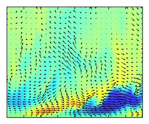
The instantaneous results highlight some of the key features in the development of the flow acceleration. Figure 5 shows the contours of the streamwise and wall-normal velocity fluctuations at  $y^{+0}=5$. The red line shows the minimum in the skin friction coefficient, which is an approximate marker for the onset of transition. In the pre-existing flow ( $x/\delta <0$), the ubiquitous near-wall streaky structures are clearly present, although the initial turbulence is of a much smaller magnitude than at the end of the acceleration. The streamwise fluctuation indicates that after the onset of the acceleration the strength of the streaks mildly increases initially and around the minimum of $C_f$ turbulent spots start to form, as indicated by the appearance of large magnitude fluctuations of shorter spatial scale. These spots are initially localised in space coexisting with the streaks but grow in the spanwise and streamwise directions as they are convected downstream until the entire wall surface is covered in new turbulence. However, the wall-normal velocity fluctuations develop differently. Figure 5(b) indicates that the wall-normal fluctuating velocity initially does not respond until the appearance of high magnitude spots, which correspond with the large magnitude events in the streamwise velocity fluctuation contour. There is a significant increase in the energy of both components on the formation of the turbulent spots, as shown by more frequent and much darker red and blue events. These observations are similar to those observed in bypass transition (e.g. Jacobs & Durbin Reference Jacobs and Durbin2001; Brandt et al. Reference Brandt, Schlatter and Henningson2004). The lack of response from $v'$ until the formation of turbulent spots is also true in boundary layer bypass transition, but the background flow in that case is laminar, hence there are few fluctuations at all. The development is nonetheless similar.

Figure 5. An  $x$–
$x$– $z$ plane of the streamwise ( $u'/U_{0}$) and wall-normal ( $v'/U_{0}$) fluctuating velocities at a single instance in time at $y^{+0}=4.9$. The first black line indicates the start of the acceleration while the final black line is the end of the acceleration. The red line indicates the approximate location of the onset of transition as indicated by the minimum in $C_f$.
We propose the following interpretation of the flow development observed above. When the mean flow is accelerated, the velocity tends to increase uniformly at all vertical locations. However, due to fluid viscosity, the flow is retarded close to the wall resulting in a new boundary layer superimposed on the existing flow, which grows downstream as the effect of the acceleration is felt farther from the wall. In the case of the relative acceleration studied here, the boundary layer is directly created by imposing a velocity on the wall. Viscosity subsequently causes the extent of the channel affected by the moving wall to increase with downstream distance. This new boundary layer initially does not significantly change the existing turbulent flow, although interactions between the existing flow and the new boundary layer characterise this initial stage of the acceleration. With the continuing growth of the boundary layer, instabilities eventually develop on localised streaks, leading to a transition to a new turbulence state. The strengthening of the streaks observed in figure 5(a) can be explained by the modulation of the pre-existing turbulent flow by the new boundary layer, which would elongate and stretch these structures extracting energy from the mean flow leading to increased  $u'$. Transition is typically marked by the occurrence of high-frequency/high-amplitude fluctuations in all three turbulence components, and this is clearly indicated by the coincident spots in the $u'$ and $v'$ velocity fluctuation contours. This is shown quantitatively later in the paper. The spread and growth of these spots can also be compared with bypass transition, where the intermittent region is linked to the coexistence of streaks and patches of broken down flow until the entire surface of the wall is covered in new turbulence structures, which is also observed here. This interpretation is analogous to the transition theory proposed by He & Seddighi (Reference He and Seddighi2013) for temporally accelerating flows. In summary, the flow can be described as a three-stage development, that is the initial pre-transition stage ( $0< x/\delta \leq 6$), the transition stage ( $6< x/\delta \leq 13$) and the fully turbulent stage ( $x/\delta > 13$). Here, the onset of transition ( $x/\delta =6$) is determined using the minimum $C_f$ and the completion of transition ( $x/\delta =13$) is the first peak in $C_f$. It should be noted that turbulence may still develop in the core of the flow after the completion of transition, which is marked by the population of new turbulence in the wall region. Such definitions are analogous to those found in studies of bypass transition (Jacobs & Durbin Reference Jacobs and Durbin2001) and temporal acceleration (He & Seddighi Reference He and Seddighi2013).
It is important to compare this interpretation with the existing understanding of spatially accelerating flows which originates from the seminal work of Narasimha & Sreenivasan (Reference Narasimha and Sreenivasan1973). As described in § 1.2, this understanding primarily centres on the initial flow laminarisation followed by a retransition to turbulence after the removal of the acceleration. The new interpretation proposes that a new boundary layer develops as the flow accelerates irrespective of laminarisation and that the transition is related to the development of this new boundary layer. This transition is thus inherently linked to the presence of the acceleration. As a result, this transition would occur even in the absence of laminarisation and potentially before the removal of the acceleration, as demonstrated in the case discussed herein. The following sections will provide more evidence to support this interpretation and how it can provide a detailed description of the moving-wall accelerating flow. The conclusion will further compare this interpretation with the theory of Narasimha & Sreenivasan (Reference Narasimha and Sreenivasan1973).
It is also useful to note the relevance of the internal boundary layer concept that has been used to describe step changes in surface roughness, temperature or humidity which has been studied particularly in the context of meteorology (Smits & Wood Reference Smits and Wood1985; Garratt Reference Garratt1990). The effect of such changes on the existing flow is often considered by the formation of an ‘internal layer’ that represents the extent of the effect of the change in boundary condition (Antonia & Luxton Reference Antonia and Luxton1971, Reference Antonia and Luxton1972; Saito & Pullin Reference Saito and Pullin2014). It should be noted that there are no discussions or observations on distinct transition behaviours in such studies. Instead, much of such work was interested in the asymptotic development of these layers.
3.3. Reynolds stresses
The streamwise distribution of the peak normal Reynolds stresses can be seen in figure 6, which illustrates the energy growth of the disturbances commonly used in studies of bypass transition. The figure shows that shortly after the start of the acceleration, the streamwise Reynolds stress exhibits downstream growth throughout pre-transition. This can be associated with the stretching and elongation of the streaks by the new boundary layer observed in figure 5 leading to an increase in the streamwise disturbance energy as energy is extracted from the mean flow. Such energy growth prior to the onset of transition is typical in bypass transition as demonstrated theoretically using transient growth theory (Andersson et al. Reference Andersson, Berggren and Henningson1999; Luchini Reference Luchini2000), and from DNS and experiment (Jacobs & Durbin Reference Jacobs and Durbin2001; Matsubara & Alfredsson Reference Matsubara and Alfredsson2001). Also consistent with the observation in figure 5(b), there is a clear lack of increase in the transverse Reynolds stresses during pre-transition. The location where the transverse Reynolds stresses begin to increase is consistent with the point of transition denoted by the minimum in  $C_f$.

Figure 6. Streamwise distribution of the peak normal Reynolds stresses normalised by  $U_{0}^2$. Here $\overline {u'u'}$ is shown on the left axis with $\overline {v'v'}$ and $\overline {w'w'}$ on the right axis. The vertical line indicates the onset of transition as indicated by the minimum in $C_f$.
The downstream growth of  $\overline {u'u'}$ prior to retransition was noted to occur in several studies of spatial acceleration such as Piomelli et al. (Reference Piomelli, Balaras and Pascarelli2000) and Bourassa & Thomas (Reference Bourassa and Thomas2009). Warnack & Fernholz (Reference Warnack and Fernholz1998) also showed that the development of the peak streamwise Reynolds stress exhibits downstream growth from near the onset of the acceleration until the onset of retransition. All of these results show that the growth of $\overline {u'u'}$ is linked to the formation of elongated streaks, which is inherently related to the presence of flow acceleration. The continuing increase in the peak streamwise Reynolds stress after the onset of transition in the present case is likely due to the acceleration continuing to extract energy from the mean flow during and post transition. Other cases, not presented here, where transition occurs after the end of the acceleration showed a slight decline in the peak streamwise Reynolds stress after transition similarly to Warnack & Fernholz (Reference Warnack and Fernholz1998). This was also observed in bypass transition (Jacobs & Durbin Reference Jacobs and Durbin2001). The wall-normal distribution of the streamwise Reynolds stress at different downstream locations is presented in figures 7(a) and 7(b). The former shows the downstream locations prior to transition, and the latter shows those after transition. Figure 7(a) indicates that during pre-transition, most of the increases in $\overline {u'u'}$ occur for $y^+<\sim 50$ and only increases further away from the wall after the onset of transition. This is consistent with Warnack & Fernholz (Reference Warnack and Fernholz1998) which also indicated that the downstream growth tends to be confined to the near-wall region in spatially accelerating flows. Figure 7(a) also indicates that the peak in the streamwise Reynolds stress moves slightly farther away from the wall, which is consistent with the thickening of the new boundary layer. This has also been observed in bypass transition (Matsubara & Alfredsson Reference Matsubara and Alfredsson2001). The same phenomenon was also observed in temporal acceleration (He & Seddighi Reference He and Seddighi2013) and in previous studies of spatial acceleration (Blackwelder & Kovasznay Reference Blackwelder and Kovasznay1972). Figure 7(b) shows that after the onset of transition, the peak streamwise Reynolds stress settles closer to the wall, consistent with the thinner boundary layer present in channel flow at higher Reynolds numbers.

Figure 7. The wall-normal distribution of the normal Reynolds stresses normalised by  $U_{0}^2$. The figures on the left (a,c,e) are of $x$ locations prior to transition and those on the right (b,d,f) are of locations after the onset of transition. The legend in (a) is used in (c) and (e) while the legend in (b) is used in (d) and (f).
Figures 7(c)–7(f) show the wall-normal distribution of  $\overline {v'v'}$ and $\overline {w'w'}$. Consistent with figure 6 and the instantaneous contour plots, figures 7(c) and 7(e) indicate that $\overline {v'v'}$ and $\overline {w'w'}$ remains almost constant through pre-transition before increasing along a broad wall-normal region after the onset of the transition. The wall-normal extent of the new turbulence continues to increase with downstream distance post-transition, and it is not until towards the end of the channel at $x/\delta \geq 21$ that there is an increase in $\overline {v'v'}$ and $\overline {w'w'}$ in the centre of the channel. This can be similarly observed in cases of bypass transition (Westin et al. Reference Westin, Boiko, Klingmann, Kozlov and Alfredsson1994; Jacobs & Durbin Reference Jacobs and Durbin2001) consistent with turbulence being diffused away from the wall as the wall-normal extent of the new boundary layer increases and is not directly linked to the formation of turbulent spots which occurs closer to the wall. Figure 8 shows $\overline {v'v'}$ normalised with respect to the local bulk (figure 8a) and friction velocities (figure 8b). This shows that with respect to local quantities, $\overline {v'v'}$ reduces, which is consistent with previous studies of spatial acceleration. After transition, with local scalings, $\overline {v'v'}$ increases which was also seen during retransition in Piomelli & Yuan (Reference Piomelli and Yuan2013).

Figure 8. The wall-normal Reynolds stress normalised by local relative bulk velocity,  $U_b$ (a) and local friction velocity, $u_\tau$ (b). The lines coloured blue are from $x$ locations after the onset of transition.
The development of the Reynolds shear stress  $\overline {u'v'}$ is shown in figure 9. During pre-transition, $\overline {u'v'}$ increases by around 60 % near the wall ( $y^+<\sim 50$). This is consistent with the delayed response of $v'$ in figure 5(b) and the increases in $u'$ being limited to the near-wall region. After transition, there are significant rises across a broad wall-normal region. Figure 9(b) indicates that the flow has largely redeveloped at $x/\delta =21$ as demonstrated by the linear distribution $\overline {u'v'}$ in the core. The frozen shear stress in the core during pre-transition is consistent with prior investigations of spatial acceleration such as Narasimha & Sreenivasan (Reference Narasimha and Sreenivasan1973) and Bourassa & Thomas (Reference Bourassa and Thomas2009). These results are consistent with Warnack & Fernholz (Reference Warnack and Fernholz1998), which similarly showed that $-\overline {u'v'}$ increases are initially limited to the near-wall region while after the onset of retransition there is a broad increase, the wall-normal extent of which increases with downstream distance. The development of $\overline {u'v'}$ shows a similar trend in bypass transition (Jacobs & Durbin Reference Jacobs and Durbin2001; Muthu & Bhushan Reference Muthu and Bhushan2020). Applying the Boussinesq hypothesis and considering the dominant strain rate only, the turbulent shear stress can be written as a product of the eddy viscosity and the velocity gradient,
 \begin{equation} {-}\overline{u'v'} = \nu_t\frac{\partial \bar{u}}{\partial y}. \end{equation}
We know (as can be inferred from the above equation) that the eddy viscosity can represent (the level of) turbulence activities and the mixing effect that turbulence brings to the flow. Figure 9(c) shows that  $\nu _t$ remains unchanged during pre-transition. This has implications for the development of the turbulent shear stress in the pre-transition region. Before the acceleration, the turbulent shear stress can be written as $-\overline {u'v'}_0 = \nu _{t0}({\partial \bar {u}_0}/{\partial y})$, and after the onset of the acceleration $-\overline {u'v'}_1 = \nu _{t1}({\partial \bar {u}_1}/{\partial y})$. Now we have observed that $\nu _{t1} = \nu _{t0}$, the change of the turbulent shear due to the acceleration, $\overline {u'v'}^\wedge$, can be given as
 \begin{equation} {-}\overline{u'v'}^\wedge{=} \nu_{t1}\frac{\partial \bar{u}_1}{\partial y} -\nu_{t0}\frac{\partial \bar{u}_0}{\partial y} = \nu_{t0}\frac{\partial \bar{u}^\wedge}{\partial y}, \end{equation}
with  $\bar {u}^\wedge$ being the additional mean flow due to the acceleration. That is, the flow perturbation $\bar {u}^\wedge$ does result in an increase in the near-wall turbulent shear stress but only as a ‘passive’ effect when it is superimposed onto the pre-existing turbulent flow. Later, we show that streamwise vorticity near the wall remains largely unchanged during the pre-transition period. We consider this an indication that the near-wall regeneration cycle is not significantly modified at this point beyond the strengthening of the near-wall streaks. After the onset of transition from $6< x/\delta <12$, figure 9(d) shows that $\nu _t$ is found to increase in a broad near-wall region, yet does not significantly increase in the core of the flow until the end of the transition phase of the acceleration. For $x/\delta \gtrsim 15$, the eddy viscosity begins increasing further from the wall with the final profile similar to the initial profile albeit with larger values. The results for the Reynolds stresses and the eddy viscosity are very similar to those of temporal acceleration, with an initial increases limited to $\overline {u'u'}$, which is followed by increases in the transverse terms and the generation of new turbulent structures with the onset of transition (He & Seddighi Reference He and Seddighi2013; Seddighi et al. Reference Seddighi, He, Vardy and Orlandi2014).

Figure 9. Reynolds shear stress,  $-\overline {u'v'}$ (a,b) normalised by $U_{0}^2$ and eddy viscosity, $\nu _t/\nu$ (c,d).
3.4. Reynolds stress budgets
The contributions to the growth of the Reynolds stresses can be analysed through the budgets of the Reynolds stress transport equation. The wall-normal distribution of the streamwise budgets normalised with respect to the wall units of the initial flow ( $u_{\tau,0}^4/\nu$) is shown in figure 10. The plot from before the onset of the acceleration at $x/\delta =0$ depicts a typical profile for wall shear flow. After the onset of the acceleration, the production exhibits streamwise growth, indicating an increase in energy being extracted from the mean flow. Such increases in production have also been noted in spatial (Bourassa & Thomas Reference Bourassa and Thomas2009) and temporal acceleration He & Seddighi (Reference He and Seddighi2013). This reflects the amplification of the streaks by the mean shear associated with the newly developing boundary layer. It is also apparent that the production rises substantially during the transition phase between $x/\delta =6$ and $x/\delta =18$. The changes in most of the terms broadly mirror that of the production except the pressure strain, which is subdued until the onset of transition. This is significant as the pressure strain is the primary redistributive mechanism between the normal Reynolds stresses and is the sole source of the wall-normal and spanwise Reynolds stress budgets. This can provide a further explanation for the delayed increases in the transverse stresses as the majority of the disturbance energy during pre-transition is produced in the streamwise component. This delay supports the notion that the changes during pre-transition are related to the strengthening of streaks which are primarily manifested in the streamwise velocity fluctuations. The results also imply that the turbulent spots observed in figure 5 are linked to energy redistribution, which is consistent with Voke & Yang (Reference Voke and Yang1995) who highlighted the importance of the pressure strain in the process of bypass transition. The delay of the process of redistribution is similarly shown in previous studies of spatial acceleration (Piomelli & Yuan Reference Piomelli and Yuan2013) and temporal acceleration (He & Seddighi Reference He and Seddighi2013). Figure 11 shows the streamwise development of some of the key terms of the wall-normally integrated streamwise Reynolds stress budget, namely the production, dissipation and pressure strain. In addition to the observations in figure 10, this figure shows that despite the large proportion of the overall increase in $\overline {u'u'}$ occurring during pre-transition, the changes of production appear significantly larger during the transition phase of the acceleration. This is consistent with the results of Jacobs & Durbin (Reference Jacobs and Durbin2001), although in this study the increase after transition is less stark due to the gradual nature of the acceleration and the relatively small velocity changes. The delayed rise of the pressure strain is also more clearly shown in this figure.

Figure 10. Streamwise Reynolds stress budget scaled with initial wall units,  $u_{\tau,0}^4/\nu$.

Figure 11. The wall-normal integral of production, pressure strain and dissipation terms of the  $\overline {u'u'}$ budget normalised by $u_{\tau 0}^4\delta /\nu$. The vertical line indicates the onset of transition as indicated by the minimum in $C_f$.
3.5. Quadrant analysis
Quadrant analysis is useful for investigating how turbulence structures change during the acceleration by looking at the different contributions (denoted  $\overline {u'v'}_Q$) to the Reynolds shear stress. The coherent motions which dominate wall shear flows tend to be ejection (Q2) events which occur when slow-moving streaks are ejected away from the wall, and sweep (Q4) events which occur when fluid rushes wall-wards to replace ejected fluid. Figure 12 presents quadrant analysis using the hyperbolic hole method of Willmarth & Lu (Reference Willmarth and Lu1972) where the contribution of each quadrant to $\overline{u'v'}$ is defined as
 $$\begin{gather} \overline{u'v'}_{Q} = \lim_{T\to\infty} \frac{1}{T}\int^T_0 u'v'I(t)\, {\rm d} t, \end{gather}$$
 $$\begin{gather}I(t) = \left\{ \begin{array}{@{}ll} 1, & (u'v')_Q \geq hu'_{rms}v'_{rms}.\\ 0, & {\rm Otherwise} \end{array} \right. \end{gather}$$
Figure 12. Plot of  $\overline {u'v'}_{Q}/\overline {u'v'}$ calculated using the method of Willmarth & Lu (Reference Willmarth and Lu1972). The values of the threshold $h$ given in the legend. The vertical dashed line indicates the onset of transition.
Figure 12 shows  $\overline {u'v'}_{Q}/\overline {u'v'}$, the proportion of the total Reynolds shear stress at different coordinates for $Q2$ and $Q4$ giving an indication of how the significance of events in these quadrants change. The larger values of $h$ indicate a higher threshold for events to be considered and, hence, shows just the stronger events contributing to the Reynolds shear stress. For typical wall shear flows, sweep events tend to dominate the near-wall region for $y^+<12$ with ejection events dominating farther from the wall. This is reflected in figure 12 where ejection events dominate at $y^{+0} =15$ and particularly at $y^{+0}=50$. It is interesting to note that the onset of transition is marked by a significant increase in the proportion of high magnitude ejection events. This is signified by similar increases in the contribution to the Reynolds shear stress across all thresholds. This also indicates that the new turbulent structures created during transition are linked to the negative $u'$ fluctuations, which is consistent with the interactions on slow-moving streaks that have been found to result in streak breakdown in bypass transition (Brandt et al. Reference Brandt, Schlatter and Henningson2004). Nolan et al. (Reference Nolan, Walsh and McEligot2010) also found a significant increase in ejection events during transition. It should be noted that the corresponding decreases in the other quadrants should not be considered an absolute reduction, but merely a reduction in their contribution compared with $Q2$ events and, as shown in figure 9(b), during transition the turbulent shear stress increases substantially. The results here can also be compared with the linear temporal acceleration of Seddighi et al. (Reference Seddighi, He, Vardy and Orlandi2014) where transition also occurred well prior to the end of the acceleration. The results in the present study are quantitatively near identical to that study, indicating that events contributing to $\overline {u'v'}$ are comparable in both studies.
Figure 13 shows that during pre-transition, the numbers of  $Q2$ and $Q4$ events both decrease, but the number of stronger events (that is, those with $h \in \{2,4\}$) tend to decrease by a smaller amount with $h=4$ remaining broadly constant. It should also be noted that the threshold in (3.4) will increase due to increasing $u'_{rms}$, indicating that the number of stronger events may even increase in absolute terms. As a result, it is likely that these events are responsible for the increases in $\overline {u'v'}$ seen in figure 9. This is supported by figure 14, which shows the mean ratio of the duration of quadrant events, $\Delta T_{Qi}$, to the interval between events, $T_{Qi}$. The steep reduction of this ratio, particularly close the wall, indicates an overall reduction in the dynamical significance of these events during pre-transition, although similarly with figure 13 this is not reflected in the stronger events. This observation is consistent with previous studies of spatial acceleration, which indicated the presence of overall fewer but stronger events (McEligot & Eckelmann Reference McEligot and Eckelmann2006; Bourassa & Thomas Reference Bourassa and Thomas2009). After the onset of transition, both the number of events and $\Delta T_{Qi}/T_{Qi}$ strongly increases with the wall-normal locations closer to wall ( $y^{+0}\in {5,15}$) responding further upstream, indicating that the processes which lead to the breakdown of the flow are linked to the dynamics of the near-wall region.

Figure 13. Number of distinct events using the method of Willmarth & Lu (Reference Willmarth and Lu1972). The vertical dashed line indicates the onset of transition.

Figure 14. The ratio of the mean duration of quadrant events and the interval between quadrant events. The vertical dashed line indicates the onset of transition.
The overall contributions to the Reynolds shear stress can be examined in more detail using joint PDFs at  $y^{+0}\in \{5,15,50\}$ and $x/\delta \in \{-3,3,9,15\}$ presented in figure 15. At the first station, the joint PDFs have the elliptical distributions typical of wall shear flows. The second station is located in the pre-transition region, which shows that the PDFs have not changed significantly, although the $u'$ distributions have been stretched consistent with the strengthening of the streaks during this region. The wall-normal distribution has barely changed, consistent with the notion of the turbulence in the transverse directions being frozen prior to transition and that the changes to the turbulent structures are primarily due to the stretching of the streaks as suggested by the new interpretation. The third downstream station is located in the transition region. During this region, the furthest station from the wall shows a large increase in high magnitude ejection events indicated by the skew towards the second quadrant. The middle station similarly shows a skew to large Q2 events and also to larger magnitude Q4 events. This is expected because at $y^{+0}=15$, the flow would experience both ejection and sweep events because, as indicated above, ejection events in typical wall shear flows tend to dominate over sweep events from $y^+>12$. Consequently, the closest station to the wall at $y^{+0}=5$ shows an increase in large magnitude sweep events. The skew present in the transition region can be explained by the intermittent nature of the flow during this region. After the onset of transition, as shown in the instantaneous contour plots, both amplified streaks and turbulent spots coexist. The spots would manifest themselves as large magnitude wall-normal events, whereas the streaks that have not undergone secondary instability have wall-normal fluctuations more consistent with the pre-existing turbulent flow. Given that these spots are the results of locally broken down flow, they are initially localised in space, and it would therefore be expected that these events would skew the joint PDFs. The significant skew towards the second quadrant particularly implicates the slow-moving streaks in the formation of the turbulent spots, which supports the results shown in figure 12. The corresponding increases in sweep events result from fluid moving wall-ward to replace the ejected fluid.

Figure 15. Joint PDF of  $u'$ and $v'$ at $y^{+0}\in \{5,15,50\}$ and $x/\delta \in \{-3,3,9,15\}$.
The PDFs from the final station, which occurs around the onset of the fully developed turbulence region, indicate that the extent of the distribution has not changed significantly from the transitional flow, but the spread has. At this station, the resulting distribution has begun to resemble a more fully developed turbulent flow.
3.6. Correlations
Figures 16 and 17 show the autocorrelation which can be used to understand how the scales of turbulent structures are altered by the acceleration. Figures 16(a) and 16(b) shows the autocorrelation with respect to spanwise and streamwise separation respectively defined as
 $$\begin{gather} R_{uu}(x,\Delta x) = \overline{u'(x) u'(x+\Delta x)}/\overline{ u'^2(x)}, \end{gather}$$
 $$\begin{gather}R_{uu}(x,\Delta z) = \overline{u'(x) u'(x,\Delta z)}/\overline{u'^2(x)}. \end{gather}$$
Figure 16(a) gives an indication of the spanwise spacing of the near-wall streaky structures. The spacing is calculated as  $2z_{min}$, where $z_{min}$ is the distance to the first minimum. After the start of the acceleration, there is a mild decrease in the absolute spanwise spacing. However, when presented in local wall units, the spacing increases during pre-transition. These results show similar trends to Talamelli et al. (Reference Talamelli, Fornaciari, Westin and Alfredsson2001), which indicated that there is a reduction in the absolute spanwise spacing, but when locally scaled, the spacing increases. These variations are substantially milder in the present study, however. Figure 16(b) shows that after the onset of the acceleration, the width of the autocorrelation increases in the streamwise direction consistent with the elongation of the streaks during pre-transition, which is related to the modulation of pre-existing structures by the new boundary layer. With the onset of transition, the correlation shortens consistent with the breakdown of the streaks and the generation of new turbulence, which is of shorter spatial scale than the initial turbulent flow as shown in figure 5(a). After the completion of transition, the streamwise scale of the turbulence is clearly far shorter than the initial flow.

Figure 16. Streamwise velocity autocorrelation in the spanwise (a) and streamwise (b) directions at various streamwise locations. The blue lines are from locations after the onset of transition.

Figure 17. A  $z$–
$z$– $y$ contour of the spanwise autocorrelation of the streamwise velocity at streamwise locations indicated in the top right of each figure. Only the values where the autocorrelation is negative are shown for clarity.
Figure 17 shows the  $z$–
$z$– $y$ contour of the spanwise autocorrelation with only the negative values present to more closely compare with similar plots in Matsubara & Alfredsson (Reference Matsubara and Alfredsson2001). Similarly to the other results in this paper, these comparisons are caveated by the differing natures of the pre-existing flow. Nonetheless, the results show a very similar trend before and during transition. It is clear that the minimum becomes more negative during the pre-transition phase consistent with a strengthening of the streaks, although the change, in general, is relatively small, consistent with a minor increase in width of the $u'-v'$ joint PDFs and the $u'$ instantaneous contour plots. After the onset of transition, the strength of the minimum clearly fades consistent with figure 16(a) due to the breakdown of the streaks during the transition phase. The development also closely resembles similar contour plots in He & Seddighi (Reference He and Seddighi2013) which showed initial strengthening in pre-transition followed by a noticeable decline in the strength of the minimum with the onset of transition.
3.7. Flow structures
With the strengthening of the streaks observed during pre-transition and the apparent role of low-speed streaks in the breakdown of the flow, it is useful to study the dynamics of the buffer layer, where these streaks reside. The near-wall turbulence is often characterised by the mutual generation and interaction of near-wall turbulent structures particularly streaks and streamwise vortices in a self-sustaining process known as the turbulence regeneration cycle (Kim Reference Kim2011). The root-mean-square of the streamwise vorticity fluctuations can be seen in figure 18 and the instantaneous streamwise vorticity can be seen in figure 19. During the pre-transition region, figure 18(a) shows that until the end on this period  $\omega '_{x,rms}$ is unchanged, which is similarly indicated by figures 19(a)–19(c). The generation of streaks is the result of the interaction between the streamwise vortices and the mean shear. The constant streamwise vorticity observed here indicates that the strengthened near-wall streaks during pre-transition are linked to the increase in the mean shear which results from the acceleration. These stronger streaks then remain stable until the onset of transition. It is conceivable that the process of generating stronger streaks through the lift-up effect may be responsible for the apparent increase in the absolute number of stronger Q2 and Q4 events observed in figure 13. The above result is consistent with those of Piomelli et al. (Reference Piomelli, Balaras and Pascarelli2000), who found that there was little change to the magnitude of the streamwise vorticity in spatially accelerating flows, although significant reorientation of the streamwise vortices was observed due to the new shear associated with the acceleration.

Figure 18. Wall-normal distribution of  $\omega '_{x,rms}$ normalised by $U_0/\delta$ at different streamwise locations: (a) during pre-transition, (b) after the onset of transition.

Figure 19. Plots of  $z$–
$z$– $y$ contours of the streamwise vorticity $\omega _x$ at different streamwise locations.
Figure 18(b) shows that with the onset of transition,  $\omega '_{x,rms}$ increases significantly until $x/\delta =15$. This can also be seen in the instantaneous plots (figure 19). Figure 19(d) shows that with the onset of transition, there are localised spots of increased streamwise vorticity, which can be seen growing downstream in figures 19(e) and 19(f). Such sudden changes can be linked to the breakdown of the streaks and are a reflection of the much smaller scales of the new turbulence structures. Figure 20 shows a top-down view of the three-dimensional isosurfaces of the streamwise velocity fluctuations and the streamwise vorticity. This figure shows the sinuous breakdown of a near-wall streak with the onset of transition in a mechanism similar to that detailed in Schoppa & Hussain (Reference Schoppa and Hussain2002). The time frame and spatial location of the plots are shifted consistently to follow the event. The low-speed streak can be seen in blue and at $t^*=71.5$, a high-speed streak (green) can be observed on the $+z$ flank of the low-speed streak. At this point, the streamwise vorticity ( $+\omega _z$ in black, $-\omega _z$ in red) isosurfaces are barely visible (under the chosen scales used here which are intended to show the regions of stronger vorticity). It is also important to note the progressive strengthening of the streaks as the downstream distance increases, which is shown by the increased volume of the isosurface. This is consistent with the streamwise autocorrelation in figure 17. At $t^*=72.5$, the strengthened positive $u'$ streak can be observed catching up with the low-speed streak with consequent generation of new streamwise vorticity. At this point, the spanwise waviness of the streaks and the patterning of the streamwise vorticity bear significant similarity to figure 25 of Schoppa & Hussain (Reference Schoppa and Hussain2002) as well as to the isosurfaces seen in Schlatter et al. (Reference Schlatter, Brandt, de Lange and Henningson2008). As the instability progresses in the subsequent frames, the spanwise waviness of $u'$ and the streamwise vorticity intensify. At $t^*=75.5$, the low-speed fluid can be seen being ejected from the near-wall region. This indicates that the generation of new localised streamwise vorticity in figure 19(d) can be linked to the breakdown of the strengthened streaks that occurs with the onset of transition. This also confirms the role of low-speed streaks in the process of transition implied by the quadrant analysis and joint PDFs. The higher energy contained in the strengthened streak makes it more susceptible to the development of instabilities on interaction with a high-speed streak. The resulting breakdown contains small scales and high magnitude disturbances characteristic of transition to a higher-Reynolds-number turbulent flow.

Figure 20. A top-down view of  $u'$ and $\omega _x$ isosurfaces at $t^*\in {70.5, 71.5, 72.5, 73.5,74.5,75.5}$; $u'$ isosurfaces $-$0.31 (blue), 0.31 (green); $\omega _x$ isosurfaces: $-$8 (red), 8 (black).
4. Summary and conclusions
In this study a novel methodology has been used to investigate an idealised spatially accelerating channel flow through the use of a longitudinally accelerating moving wall in order to understand the response of turbulence to bulk flow acceleration. A new interpretation has been developed to explain this accelerating flow which can be summarised as follows: following the commencement of the acceleration, a new boundary forms superimposed on the existing turbulent flow. The development of this boundary layer and the eventual transition of the flow in response to its development can explain the turbulence dynamics of the accelerating flow. The transition identified herein, which is inherently linked to the presence of the acceleration, is believed to be a generic feature of spatially accelerating flows, though this proposition and any detailed flow behaviour needs further investigation with more practical flow configurations.
4.1. Summary of flow development and evidence for the interpretation
At the onset of the acceleration, a thin boundary layer is formed at the wall, which develops with downstream distance. This boundary layer modulates the pre-existing turbulent structures such as the streaks, which are stretched and elongated as indicated by the streamwise autocorrelation. This results in the extraction of energy from the mean flow and the consequent growth of the streamwise disturbance energy. The eddy viscosity during this region remains largely unchanged, which indicates that the changes in turbulent shear stress can be related solely to the increasing mean shear associated with the superimposition of the boundary layer onto the pre-existing turbulent flow. Consistent with this, the pressure strain remains largely unchanged indicating that there is no additional transfer of energy from the strengthening  $u'$ to $v'$ and $w'$. In this initial phase of the acceleration, the fundamental turbulence characteristics are not significantly altered. This region occupies $0< x/\delta \leq 6$ and is described as pre-transition.
The pre-transition region is terminated by the formation of turbulent spots as the amplified low-speed streaks become unstable. As indicated by the instantaneous plots of  $u'$ and $v'$, the spots grow in the spanwise and streamwise directions as they are convected downstream until they merge, resulting in a fully turbulent region. These spots appear to originate from specific streaks similarly to bypass transition. The quadrant analysis indicates that the spots are linked to extreme ejection events consistent with the breakdown of low-speed streaks, which is supported by instantaneous plots detailing the strengthening and breakdown of a single streak reminiscent of the sinuous breakdown mechanism seen in near-wall turbulent flows. At this point, the pressure strain begins to increase, resulting in the redistribution of energy to the transverse Reynolds stresses, which until this point had been frozen. The effect of the turbulent spots on the transverse terms appears to occur simultaneously over a broad wall-normal region. The coexistence of the spots with the streaks, which also occurs in the intermittent region of boundary layer bypass transition, is indicated by the joint PDFs of $u'$ and $v'$, and the instantaneous contour plots.
After the merging of the turbulent spots, the acceleration enters the fully turbulent region. This region is characterised by the diffusion of turbulence in the wall-normal direction as the initial turbulence is generated closer to the wall and only subsequently spreads into the core. The flow in the near-wall region does not change significantly during this phase of the acceleration.
While it is evident that a process akin to transition occurs as a result of the acceleration, some differences between the present flow and the bypass transition of a laminar boundary layer need to be highlighted. A key difference is the nature of the pre-existing turbulence. In bypass transition, the pre-existing flow is typically homogeneous and isotropic with low frequencies penetrating the boundary layer through receptivity, leading to the formation of streaks which are amplified by the mean shear. It is also often a source of streak secondary instability. In the present case, the pre-existing flow is an inhomogeneous, anisotropic wall shear flow containing structures with broad frequencies which interact with the new boundary layer. The larger streamwise structures are amplified by the mean shear and later undergo secondary instability. These differences have also been highlighted in studies of temporal acceleration (He & Seddighi Reference He and Seddighi2013) and a more detailed understanding of the nature of these interactions in accelerating flows should be an aspect of future study.
4.2. Comparison of the new interpretation with Narasimha & Sreenivasan (Reference Narasimha and Sreenivasan1973)
It is useful to compare the new interpretation with the existing theory of laminarisation in spatially accelerating flows summarised using the four stages described in Narasimha & Sreenivasan (Reference Narasimha and Sreenivasan1973), shortened as NS1973 hereafter. It should be noted that while other detailed explanations of the laminarisation process have been proposed, NS1973 largely remains the framework for the understanding of such flows. Figure 21(a) shows a schematic of the new interpretation with the linear acceleration of the present case depicted. Figure 21(b) shows a schematic of the theory from NS1973. The existing theory explains the flow development in terms of the development of the existing boundary layer. Initially, the boundary layer would retain its existing turbulence characteristics (region I) before beginning to exhibit progressively more laminar-like qualities (region II) until region III, where the flow can be considered quasi-laminar. At this stage, the turbulent stresses (or the turbulent transport term as in Dixit & Ramesh (Reference Dixit and Ramesh2010)) are relatively small in comparison to the substantially increased mean flow and, hence, do not significantly affect the mean flow dynamics. After the removal of the acceleration, the boundary layer retransitions to turbulence (region IV). Narasimha & Sreenivasan (Reference Narasimha and Sreenivasan1973) developed a model successfully treating the inner layer for region III as laminar while treating region I as turbulent. Neither modelling approaches were able to predict region II.

Figure 21. Comparison of the new interpretation with the theory of Narasimha & Sreenivasan (Reference Narasimha and Sreenivasan1973). (a) The new interpretation with its regions marked. (b) The theory of Narasimha & Sreenivasan (Reference Narasimha and Sreenivasan1973) with its four stages marked. The solid line in both plots represents the streamwise velocity. The dashed line in (a) is the thickness of the new boundary layer developing in response to the acceleration. The dashed line in (b) represents the boundary layer thickness of the full flow.
In the new interpretation proposed herein, regions I to III correspond with the initial pre-transition phase of the acceleration and region IV is associated with the transition and fully turbulent stages. In regions I to III, studies of spatial acceleration have shown, although frequently not emphasised, the significantly different behaviours of the streamwise and the two transverse components of the turbulence and these can be associated with typical pre-transitional flow characteristics as described in the paper. In the new interpretation, the transition is related to the development of instabilities that result from the development of the new boundary layer and is thus inherent to the presence of the acceleration itself. As a result, this transition is not necessarily linked to the end of the acceleration as found in the flow studied herein.
4.3. Comparison between moving-wall flow and conventional acceleration
The moving-wall flow shares many characteristics as well as some differences with conventional spatially accelerating flows. Among the similarities are the downstream growth of  $\overline {u'u'}$ from the commencement of the acceleration, which has been widely observed in previous studies of spatial acceleration, and the contrasting behaviour of the transverse components, which remain largely frozen during this period. When normalised with local scalings, the transverse terms exhibit a reduction which is typical in spatially accelerating flows. The behaviour of the Reynolds shear stress is also similar, with substantial growth in the near-wall region during pre-transition and freezing farther away. Following the onset of transition, the growth of this quantity closely matches the trends observed in the experiments of Warnack & Fernholz (Reference Warnack and Fernholz1998). The increasing trend in the turbulence production and the constant pressure strain in pre-transition are also consistent with previous studies. The minimum and maximum of $C_f$ and $H$, respectively, broadly coincide with the onset of transition which has also been found in spatially accelerating flows (Escudier et al. Reference Escudier, Abdel-Hameed, Johnson and Sutcliffe1998). The quadrant analysis also shows that the contribution of stronger events to the Reynolds shear stress increases during pre-transition, which has been shown by many previous studies (McEligot & Eckelmann Reference McEligot and Eckelmann2006; Bourassa & Thomas Reference Bourassa and Thomas2009).
Despite these similarities, there are some important differences between the moving-wall flow and more conventional spatial accelerations. The most significant difference is the reduced variation of the von Kármán constant,  $\kappa$, which seems to be due to the lack of contraction effects. The contraction inherent to more conventional spatial accelerations is likely to cause the flow to be skewed towards the wall, resulting in a stronger increase in velocity closer to the wall than further away from it and, hence, larger changes in $\kappa$ and, to some extent, $B$. In support of the above reasoning, the changes in the logarithmic law in the present study show a similar trend to those of accelerations without a ward-wards contraction, including, for example, the spatial acceleration in laterally converging ducts of McEligot & Eckelmann (Reference McEligot and Eckelmann2006) and the temporal acceleration of Seddighi et al. (Reference Seddighi, He, Vardy and Orlandi2014). In order to understand such effects and their impact on turbulence development, comparisons between the moving-wall and conventional accelerations are required and will be an aspect of future work. The lack of contraction in the present flow has also enabled some comparisons with previous studies of temporal acceleration. Indeed, much of the conclusions described in § 4.1 for the moving-wall flow are similar to those observed in temporal acceleration. This is significant given that the origins of the new interpretation lie with the theory for temporal acceleration first proposed in He & Seddighi (Reference He and Seddighi2013).
Table 2. Details of turbulence generator.
Acknowledgements
The authors thank Dr W. Wang for her support with respect to the development and use of CHAPSim DNS code. The authors would also like to thank the anonymous reviewers for their insightful comments, which resulted in a substantially improved manuscript.
Funding
This research was supported by HPC resources from the UK Turbulence Consortium (grant no. EP/R029326/1) and received technical support from CCP NTH (grant no. EP/T026685/1). M.F. was also supported by the University of Sheffield's Department of Mechanical Engineering EPSRC Doctoral Training Partnership.
Declaration of interests
The authors report no conflict of interest.
Appendix A. Details of the turbulence generator
As stated in § 2, a turbulence generator is used to provide a fully turbulent inlet for the moving-wall acceleration. The domain size, mesh and resolution are shown in table 2. The streamwise velocity profile and the root-mean-square velocity fluctuations are shown in figure 22 compared with channel flow at  $Re_\tau =180$ from the DNS database of Vreman & Kuerten (Reference Vreman and Kuerten2014). This shows that the turbulent statistics produced by the turbulence generator agree closely with existing results. Figure 23 shows the streamwise autocorrelation in the periodic streamwise and spanwise directions. These plots show that by the half-width and half-length of the channel, the correlation is close to zero indicating that the turbulence generator size is sufficient.

Figure 22. Comparison of the turbulence generator (lines) with Vreman & Kuerten (Reference Vreman and Kuerten2014) (markers): (a)  $\bar {u}^+$ vs $y^+$, (b) ${(\overline {u^{\prime +}_i})}_{rms}$ vs $y^+$.

Figure 23. Streamwise autocorrelation for turbulence generator at  $y^+\in \{5, 15,50,150\}$. (a) Spanwise direction. (b) Streamwise direction.
Appendix B. Moving-wall acceleration with a smooth and gradual flow increase
Some results are presented below of a smooth acceleration which show that the overall phenomena, including most significantly the location of transition, are largely unchanged compared with the linear acceleration presented in the main body of the paper. In order to create an equivalent smooth acceleration a  $\tanh$ function was used such that the acceleration, ${\rm d}U/{{\rm d}\kern0.06em x}$, in the middle of the acceleration is the same as the linear case and the velocity of both cases was the same in the middle of the acceleration. Enforcing these conditions results in
 \begin{equation} U(x) = U_0 - U_w(x) = U_0 + \frac{\Delta U}{2} \left[\tanh \left(\frac{2x}{\Delta x} + 1\right) + 1\right], \end{equation}
where  $x$ is the downstream distance from the nominal onset of the acceleration in the equivalent linear case. Here $\Delta x$ is the streamwise length of the acceleration in the equivalent linear acceleration case. The resulting bulk velocity profile and acceleration parameter distributions for the smooth case compared with the case presented in the study are shown in figure 24. It can be seen that the peak $K$ observed in figure 4 is now absent in the ‘smooth’ case, which shows a shape more similar to those exhibited in conventional flows. Figure 25 shows that the general behaviour of the skin friction coefficient and shape factor in the two cases are similar. In particular, the locations of the minimum $C_f$ and peak $H$ are similar in the two flows, which indicates that the smoothing of the flow acceleration profile does not change the key transition features of the flows presented in the main body of the paper. The parameters in figure 25 show some detailed different behaviour prior to transition, which can be explained by the longer acceleration in the smooth case. Preliminary results from $\overline {u'u'}_{max}$ and $\overline {v'v'}_{max}$ (not presented) also show similar trends to the results presented in the paper.

Figure 24. Smooth case compared with the case presented in the paper. (a) Relative bulk velocity. (b) Acceleration parameter.

Figure 25. Smooth case compared with the case presented in the paper. (a) Skin friction coefficient. (b) Shape factor.


 Open access