


1. Introduction
Laminar–turbulent transition can induce huge variations of skin friction and heat transfer, and is therefore very important in designing hypersonic vehicles. While transition mechanisms of essentially two-dimensional (2-D) boundary layers of simple configurations (such as a flat plate, a concave wall, a circular cone at zero angle of attack) have been well studied (Mack Reference Mack1984; Fedorov Reference Fedorov2011; Schneider Reference Schneider2015), investigation of stability of three-dimensional (3-D) boundary layers, in which two essentially inhomogeneous spatial directions exist, is still in its infancy stage. Since 3-D boundary layers are more relevant in hypersonic flights, the related transition problem receives ever growing attention despite significantly increased complexity compared to its 2-D counterpart. Typical configurations utilized in studying 3-D boundary layer transition include circular cones with non-zero angles of attack, elliptic cones (say HIFiRE-5 model, Kimmel, Adamczak & Juliano Reference Kimmel, Adamczak and Juliano2013), the BoLT model (Wheaton et al. Reference Wheaton, Berridge, Wolf, Araya, Stevens, McGrath, Kemp and Adamczak2020) and the lifting body (the Hypersonic Transition Research Vehicle, HyTRV) (Chen et al. Reference Chen, Tu, Wan, Yuan, Yang, Zhuang and Xiang2021). The most prominent feature of 3-D boundary layers is notable azimuthal pressure gradients that transport fluid from the high-pressure region to concentrate in the low-pressure region. As a result, 3-D boundary layers generally consist of three distinct unstable regions, that is, the attachment-line region near the high-pressure region, the (streamwise) vortex region in the vicinity of the low-pressure region, and the cross-flow region in between. Below we give a brief summary of previous studies on these three flow regions.
Through extensive studies, good knowledge has been obtained for stability characteristics of streamwise vortices on different configurations, such as an elliptic cone (Choudhari et al. Reference Choudhari, Chang, Jentink, Li, Berger, Candler and Kimmel2009; Juliano & Schneider Reference Juliano and Schneider2010; Paredes et al. Reference Paredes, Gosse, Theofilis and Kimmel2016; Li et al. Reference Li, Zhang, Liu, Huang, Luo and Zhang2018; Choudhari, Li & Paredes Reference Choudhari, Li and Paredes2020), BoLT (Berridge et al. Reference Berridge, Kostak, McKiernan, King, Wason, Wheaton, Wolf and Schneider2019; Knutson, Thome & Candler Reference Knutson, Thome and Candler2019; Kostak & Browersox Reference Kostak and Browersox2020; Li, Choudhari & Paredes Reference Li, Choudhari and Paredes2020a) and a yawed cone (Chen et al. Reference Chen, Chen, Dong, Xu and Yuan2020; Li et al. Reference Li, Chen, Huang, Yang and Xu2020b). Streamwise vortices would greatly distort the profiles in the cross-section, forming mushroom structures with multiple high-shear layers. Substantial variations in the azimuthal direction render the failure of one-dimensional (1-D) stability analyses (linear stability theory, LST and parabolized stability equations, PSE) and the necessity of multi-dimensional stability analyses (BiGlobal and PSE3D). Each high-shear layer likely supports one or several unstable modes, which ultimately lead to the breakdown of streamwise vortices. Unstable shear-layer modes can be further classified as odd (sinuous) and even (varicose) modes according to the spanwise symmetry, or inner and outer modes according to the spatial distribution, or Y and Z modes according to the dominant energy production. Which type of mode dominates the transition process depends on the specific flow configurations.
In a cross-flow region, the cross-flow velocity profile has an inflectional point, and is thereby conducive to the cross-flow instability (Saric, Reed & White Reference Saric, Reed and White2003). In addition, oblique (second) Mack modes, rather than the planar counterpart that is typically more unstable in 2-D boundary layers, are likely present (Balakumar & Reed Reference Balakumar and Reed1991). Base flow in the cross-flow region varies relatively slightly in the azimuthal direction, hence 1-D stability analyses appear to be amenable. In order to obtain the evolution of cross-flow vortices, a common practice is to first model a vortex path and the azimuthal wavenumber variation along the path, and then integrate the nonlinear parabolized stability equations (NPSE) with assumption of azimuthal periodicity (Oliviero et al. Reference Oliviero, Kocian, Moyes and Reed2015; Kocian et al. Reference Kocian, Moyes, Mullen and Reed2017; Moyes et al. Reference Moyes, Kocian, Mullen and Reed2017a,Reference Moyes, Paredes, Kocian and Reedb). However, there still exist some difficulties. First, how to accurately predict the disturbance trajectory and the azimuthal wavelength variation along the trajectory are still open to question, although some progress has been made recently (Kocian et al. Reference Kocian, Moyes, Reed, Craig, Saric, Schneider and Edelman2019). Second, nonlinear interactions among multiple modes, which is essential in understanding the transition mechanism, cannot be tackled by local analyses since local modes may have different trajectories and thus may not interact. Third, unstable modes generally exhibit a wavepacket structure in the azimuthal direction, which is hard to model by 1-D stability analyses. These difficulties would be overcome by multi-dimensional stability analyses. A major drawback of multi-dimensional stability analyses is their large time and storage consumption (Tullio et al. Reference Tullio, Paredes, Sandham and Theofilis2013), especially for the cross-flow mode, whose wide spatial distribution and small wave scale require a large number of azimuthal grid points (about  $O(1000)$) to resolve. As far as the authors know, only Paredes et al. (Reference Paredes, Gosse, Theofilis and Kimmel2016) and Lakebrink, Paredes & Borg (Reference Lakebrink, Paredes and Borg2017) have investigated cross-flow instabilities via BiGlobal analysis for the HIFiRE-5 elliptic cone, and, in particular, the latter have observed notable discrepancies in growth rates between BiGlobal and LST results.
Extensive experimental studies have also been conducted to trace evolution of cross-flow vortices, to reveal possible nonlinear modal interactions, to clarify effects of freestream disturbances and surface inhomogeneity, and to explore transition control approaches (Borg, Kimmel & Stanfield Reference Borg, Kimmel and Stanfield2011, Reference Borg, Kimmel and Stanfield2012, Reference Borg, Kimmel and Stanfield2013; Borg et al. Reference Borg, Kimmel, Hofferth, Bowersox and Mai2015; Ward, Henderson & Schneider Reference Ward, Henderson and Schneider2015; Craig & Saric Reference Craig and Saric2016; Lakebrink & Borg Reference Lakebrink and Borg2016; Corke et al. Reference Corke, Arndt, Matlis and Semper2018; Neel, Leidy & Bowersox Reference Neel, Leidy and Bowersox2018; Arndt et al. Reference Arndt, Corke, Matlis and Semper2020). Several important results are listed below. First, stationary and travelling cross-flow vortices coexist in both quiet (low-noise conditions) and conventional (high-noise conditions) wind tunnels, and their interactions are also detected. Second, stationary cross-flow vortices are dominant for quiet flow, whereas travelling cross-flow waves are more relevant for noisy flow. Third, interactions between stationary and travelling cross-flow modes, and interactions between Mack instabilities and cross-flow vortices, likely coexist, and it is hard to distinguish experimentally between Mack instabilities and secondary instabilities of cross-flow vortices.
Many studies have focused on the transition process of cross-flow vortices in 3-D boundary layers with help of numerical simulations. Boundary layer transition induced by roughness (Balakumar & Owens Reference Balakumar and Owens2010; Choudhari, Li & Paredes Reference Choudhari, Li and Paredes2017) or by random blowing and suction immediately downstream of the tip (Dong et al. Reference Dong, Chen, Yuan, Chen and Xu2020) over a straight cone at non-zero angle of attack and Mach number 6 have been computed. Roughness can effectively trigger stationary cross-flow vortices, whereas blowing and suction tend to induce travelling cross-flow vortices. Therefore, the transition pattern of the former is similar to experimental observation in quiet wind tunnels, while the latter is more like noisy cases. Nevertheless, Mack modes are observed to be substantially destabilized by cross-flow vortices in both cases. Dinzl & Candler (Reference Dinzl and Candler2015) emphasized the necessity of carefully considering the grid distribution and numerical schemes to obtain disturbance-free laminar flow for the HIFiRE-5 elliptic cone. They subsequently (Dinzl & Candler Reference Dinzl and Candler2017) conducted direct numerical simulation (DNS) of evolution of stationary cross-flow vortices excited by the distributed roughness near the nose of the cone, and observed similar heat flux streak patterns as observed in experiments. Recently, Tufts et al. (Reference Tufts, Borg, Bisek and Kimmel2020) performed high-fidelity simulations of HIFiRE-5 boundary layer transition. Their results suggested that travelling cross-flow waves may play a significant role in transition processes under both low- and high-freestream disturbances.
In the vicinity of an attachment line, the streamlines diverge and the boundary layer exhibits non-negligible variations of the base flow components with respect to the azimuthal direction. Studies of attachment-line transition have been conducted mostly in the context of incompressible and compressible flows with moderate Mach numbers over swept wings or cylinders (see, for example, Gennaro et al. (Reference Gennaro, Rodriguez, Medeiros and Theofilis2013), and references therein). Investigations on hypersonic attachment-line boundary layer transition over 3-D configurations are relatively scarce. Borg et al. (Reference Borg, Kimmel and Stanfield2011) examined experimentally the critical roughness height for the leading edge boundary of the HIFiRE-5 configuration. The critical roughness height is defined as the minimum roughness height that first causes transition to move forward relative to the smooth-wall transition location for both 2-D and 3-D roughness geometries. It is found that the critical roughness height remarkably increases when the freestream noise decreases from noisy to quiet levels. However, they did not observe the natural attachment-line transition under quiet-flow conditions. Attachment-line transition occurred under noisy-flow conditions in several ground tests, which is always the most downstream point in the transitional front and appears to be due to contamination from the outboard transition (Tufts, Gosse & Kimmel Reference Tufts, Gosse and Kimmel2017). A distinct attachment-line transition lobe seems to be observed only in tests performed at CUBRC, where the wall temperature ratio closely approximates flight conditions (Holden et al. Reference Holden, Wadhams, MacLean and Mundy2009; Tufts et al. Reference Tufts, Gosse and Kimmel2017). Paredes et al. (Reference Paredes, Gosse, Theofilis and Kimmel2016) performed BiGlobal stability analysis on the HIFiRE-5 attachment-line boundary layer. They found that symmetrical and antisymmetrical Mack modes alternatively emerge in the spectrum. Their results also indicate that the connection between attachment-line instabilities and cross-flow instabilities, as suggested in incompressible cases (Mack, Schmid & Sesterhenn Reference Mack, Schmid and Sesterhenn2008), no longer exists in their case.
Despite the progress made above, some questions still remain. First, detailed transition information of 3-D boundary layers in terms of flow structures, disturbance spectrum and amplitude evolution is lacking. Second, systematic multi-dimensional stability analyses over the whole 3-D model accounting for streamwise non-parallel effects, and their verification with numerical simulations, have not yet been reported. Third, boundary layer instabilities for a more realistic configuration where streamwise vortices and the attachment-line base flow may lose symmetry remain largely unknown. The lifting-body shape of the HyTRV model resembles typical hypersonic vehicles, and is generated by analytical functions that are easy to share with the community. Chen et al. (Reference Chen, Tu, Wan, Yuan, Yang, Zhuang and Xiang2021) have performed a parametric study of the HyTRV model under various angles of attack, regarding the base flow features and linear stability characteristics via 1-D stability analyses. Upon the completion of the present study, we came across the recently published work by Qi et al. (Reference Qi, Li, Yu and Tong2021), who numerically simulated the boundary layer transition over the HyTRV model under typical wind tunnel conditions, and performed the proper orthogonal decomposition analysis for the shoulder vortical region. In this paper, large-scale numerical simulations with up to 3.1 billion grid points were performed to capture the transition process of the HyTRV model with nominally the same flow conditions except for the angle of attack as Qi et al. (Reference Qi, Li, Yu and Tong2021). Systematic multi-dimensional stability analyses that take into account curvatures and streamwise boundary layer growth were then carried out to reveal the dominant transition mechanisms on some selected regions of interest and to serve as a cross-verification with numerical simulation results. Particular attention will be paid to instabilities in cross-flow regions where theoretical results are few in the literature.
The paper is organized as follows. The numerical settings and multi-dimensional stability theories are introduced in § 2. Results of numerical simulation and stability analyses are presented in § 3. A summary and concluding remarks are offered in § 4.
2. Numerical settings and linear stability theory
The numerical simulation and stability analysis are based on the equations of ideal gas flow written in dimensionless form as
 \begin{gather} \frac{\partial\rho}{\partial t} + \boldsymbol{\nabla}\boldsymbol{\cdot}(\rho \boldsymbol{V}) = 0, \end{gather}
 \begin{gather}\rho\left[\frac{\partial \boldsymbol V}{\partial t} + (\boldsymbol V\boldsymbol{\cdot} \boldsymbol\nabla)\boldsymbol V\right] ={-}\boldsymbol\nabla p + \frac{1}{R}\boldsymbol\nabla\boldsymbol{\cdot} \left[\mu\left(\boldsymbol\nabla\boldsymbol V + \boldsymbol\nabla\boldsymbol V^t -\frac{2}{3}\boldsymbol\nabla\boldsymbol{\cdot} \boldsymbol V \boldsymbol I\right)\right], \end{gather}
 \begin{gather} \rho\left[\frac{\partial T}{\partial t} + (\boldsymbol V\boldsymbol{\cdot} \boldsymbol\nabla)T\right] = (\gamma-1)M^2\left[\frac{\partial P}{\partial t} + (\boldsymbol V\boldsymbol{\cdot} \boldsymbol\nabla)P\right] + \frac{1}{RPr}\boldsymbol\nabla\boldsymbol{\cdot} (\kappa\boldsymbol\nabla T) \nonumber\\ \quad +\frac{(\gamma-1)M^2\mu}{2R}\left(\boldsymbol\nabla\boldsymbol V + \boldsymbol\nabla\boldsymbol V^t -\frac{2}{3}\boldsymbol\nabla\boldsymbol{\cdot} \boldsymbol V \boldsymbol I\right):\left(\boldsymbol\nabla\boldsymbol V + \boldsymbol\nabla\boldsymbol V^t -\frac{2}{3}\boldsymbol\nabla\boldsymbol{\cdot} \boldsymbol V \boldsymbol I\right), \end{gather}
where  $\boldsymbol V = (U,V,W)$ is the velocity vector, $\boldsymbol I$ is the identity tensor, $\rho$ is the density, $P$ is the pressure, $T$ is the temperature, $M$ is the Mach number, $R$ is the Reynolds number, $Pr = 0.7$ is the Prandtl number, $\gamma = 1.4$ is the specific heat coefficient, $\kappa$ is the thermal conductivity and $\mu$ is the first coefficient of viscosity. The reference values of velocity and temperature are the corresponding values at the free stream with the subscript $\infty$. The reference value for pressure is $\rho_\infty^*U_\infty^{*2}$. The equation of state is $p = \rho T/(\gamma M^2)$. Stokes’ law has been assumed, and the viscosity coefficient is estimated by Sutherland's law
 \begin{equation} \mu = T^{3/2}\,\frac{1+Cs}{T+Cs}, \end{equation}
with  $Cs = 110.4 K/T^*_\infty$ for air in standard conditions. The dimensional variables are denoted with the superscript $*$.
$*$.
2.1. The HyTRV model and flow conditions
The HyTRV model and coordinates are sketched in figure 1. The detailed geometry information can be found in Liu et al. (Reference Liu, Yuan, Liu, Yang, Tu, Chen, Gui and Chen2021). The model's head is an elliptic cone with aspect ratio 2 : 1. The body cross-section is generated separately in the windward and leeward sides. The windward part is an aspect ratio 4 : 1 elliptic cone, while the leeward part is a linear combination of a class function and shape function transformation technique (CST) curve and an elliptic curve with aspect ratio 4 : 1. The generation function for the leeward curve in the bottom cross-section is
 \begin{gather} z = \cos\theta W, \end{gather}
 \begin{gather}y = (1-\chi)\underbrace{[(1+\cos\theta)^4(1-\cos\theta)^4]H_l}_{\text{CST curve}} + \chi\underbrace{\sin\theta H_w}_{\text{elliptic curve}},\quad \theta \in [0,{\rm \pi}], \end{gather}
where  $W$ is the half-width of the cross-section, $H_l$ is the leeward height, $H_w\equiv 1/4W$ is the windward height and $\chi \equiv (1-H_w/H_l)$ to assure local azimuthal symmetry with respect to the shoulder line. Here, $\theta$ is a parameter ranging from 0 to ${\rm \pi}$ and has no geometric meaning. The head and bottom of the model connect by a straight line so that the streamwise slope remains continuous. The whole length is 1600 mm. The angle of attack is $2^\circ$. Typical Mach 6 wind tunnel flow conditions are used, i.e. static temperature 79 K, unit Reynolds number $10^7$ m $^{-1}$, and wall temperature 300 K. The Cartesian coordinates are represented by $(X, Y, Z)$, and $(U,V,W)$ are corresponding velocity components. The body-oriented coordinates are represented by $(\xi, \delta, \phi )$, where $\xi \equiv X$ denotes the axial coordinate, $\delta$ the wall-normal coordinate and $\phi \equiv \arctan Y/Z$ the azimuthal angle coordinate.
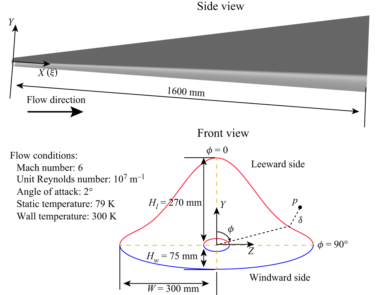
Figure 1. Front and side views of the HyTRV model. The inflow conditions, the Cartesian coordinate system  $(X,Y,Z)$ and the body-oriented coordinate system $(\xi,\delta,\phi )$ are also shown ( $X\equiv \xi$).
2.2. Numerical simulations
The parallel computational fluid dynamics software OPENCFD, developed by (Li, Fu & Ma Reference Li, Fu and Ma2008), was used for the numerical simulation. The simulation strategy consists of two steps. First, the steady base flow of the entire model is computed using the finite-volume algorithm with a second-order accurate scheme, as a laminar simulation. In the second step, the calculated steady flow serves as initial and out-boundary conditions for the laminar and transition simulations that are both performed for a smaller block  $(X^* \in [30\ {\rm mm},1600\ {\rm mm}])$ downstream of the nose part. The laminar simulation is aimed at obtaining the adequately resolved laminar boundary layer for stability analysis. The convective and viscous terms are discretized with a fifth-order accurate upwind scheme and a sixth-order accurate central difference scheme. Exploiting the symmetry of the HyTRV geometry, only half of the model is modelled with symmetry boundary conditions being forced in the leeward and windward centrelines. The computational domain is resolved using 520, 741 and 241 nodes in the streamwise, azimuthal and wall-normal directions, respectively. The azimuthal grid points are distributed in a manner such that more points lie in the regions where streamwise vortices are expected to be present. Compared with the previous DNS study on a similar configuration (Chen et al. Reference Chen, Tu, Wan, Yuan, Yang, Zhuang and Xiang2021), the basic flow can be adequately resolved under this grid resolution.
In the transition simulation, the inviscid fluxes are computed by using a seventh-order weighted essentially non-oscillatory (WENO) finite difference scheme, while the viscous fluxes are discretized using a sixth-order central difference scheme. The time integration is performed using a third-order Runge–Kutta scheme.
Blowing and suction fluctuations are introduced continuously into the boundary layer. The forcing amplitude is given by
 \begin{equation} A(x,\phi,t) = A_0(2r(\phi)-1)\sin^3({\rm \pi}(x^*-x_1^*)/(x_2^*-x_1^*)), \end{equation}
where  $A_0$, equal to 0.1 % of streamwise velocity, is the maximum forcing amplitude, $r\in [0, 1]$ is a pseudorandom number generated at every time step for each azimuthal point, and $x_1^* = 90$ mm, $x_2^* = 100$ mm. By forcing stochastically, the initial perturbations contain a broad spectrum of frequencies and azimuthal wavenumbers (see also Li, Fu & Ma Reference Li, Fu and Ma2010; Knutson et al. Reference Knutson, Thome and Candler2019). The grid system has 3000 axial grid points, 3200 azimuthal grid points, and 161 wall-normal grid points, resulting in a total of 1.55 billion points. The grid distribution in the axial direction is adjusted so that more points are distributed in the region of $X^*\in [800~{\rm mm} ,1300~{\rm mm}]$ where most of the instabilities reside; see figure 2( $a$). Furthermore, the mesh sizing increases approaching the rear part of the model, diminishing the fluctuation reflection from the outlet. Because the flow configuration is symmetrical with respect to the leeward centreline ( $\phi = 0$) and the windward centreline ( $\phi = 180^\circ$), we need to examine the boundary layer transition over only half of the lifting body. On the other hand, instantaneous fluctuations are not symmetrical at these centrelines, hence employing symmetry boundary conditions is inappropriate. Here, 3100 points are distributed in the azimuthal direction from $\phi =-22.5^\circ$ to $\phi = 202.5^\circ$, with equal spacings in $\phi$, and another 100 points cover the rest interval (coarse-grid region), with spacings being increased away from the fine-grid region, as depicted in figure 2( $b$). Such a distribution strategy of azimuthal grid points proved to achieve a good balance between accurately capturing the boundary layer transition process and minimizing the computational cost (Li et al. Reference Li, Fu and Ma2008, Reference Li, Fu and Ma2010). The boundary layer is resolved by at least 80 grid points in the wall-normal direction for most of the lifting body, and the first-layer spacing in wall unit, ${\rm \Delta} y^+_{{min}}$, is below 0.45. Detailed grid resolution presented in Appendix A shows that the flow upstream of the late transition stage is fully resolved with respect to DNS standards, except for the attachment-line instabilities. When the flow becomes turbulent and the wall-shear stress is maximum, the boundary layer based on this mesh sizing becomes slightly under-resolved and the resolution is in between the typical LES and DNS resolutions (Garnier, Adams & Sagaut Reference Garnier, Adams and Sagaut2009; Lugrin et al. Reference Lugrin, Beneddine, Leclercq, Garnier and Bur2021). Therefore, the computation corresponds to a quasi-direct numerical simulation (QDNS, such as defined by Spalart Reference Spalart2000). In this paper, our aim is to capture the evolution of linear instabilities preceding the transition, hence the resolution is sufficiently fine. Grid convergence is partially performed by doubling the grid points in the axial direction, leading to a total of 3.1 billion points. The results indicate that the transitional flow pattern remains the same; see Appendix A.
Figure 2. Grid distribution for the transition simulation. ( $a$) Axial grid distribution. ( $b$) Sketch of the mesh grid on a cross-section. For clarity, every fifth grid point is shown in the fine-grid region $\phi \in [-22.5, 202.5]^\circ$.
2.3. BiGlobal method
The stability analysis is performed on the body-oriented coordinate system. We consider the stability characteristics in the cross-section by decomposing the flow field as
 \begin{equation} \boldsymbol{q}(\xi,\delta,\phi,t) = \bar{\boldsymbol q}(\delta,\phi) +\boldsymbol{q'}(\xi,\delta,\phi,t) = \bar{\boldsymbol q}(\delta,\phi) \!+\! \epsilon\,\hat{\boldsymbol q}(\delta,\phi)\exp({\rm i}\alpha\xi \!-\! {\rm i}\omega t) \!+\! {\rm c.c.}, \quad \epsilon \!\ll\! 1, \end{equation}
where  $\boldsymbol q = (U,V,W,P,T)^t$, $\bar {\boldsymbol q}$ are the basic states, $\boldsymbol {q'}$ are the infinitesimal perturbations, $\hat {\boldsymbol q}$ is the shape function of the disturbances and $\alpha$ represents the axial wavenumber; $\omega$ is the angular frequency, with the corresponding frequency denoted by $f$. After substituting the above decompositions into the Navier–Stokes equations, subtracting the basic states and neglecting the non-parallel and nonlinear terms, one obtains the eigenvalue problems as
 \begin{equation} \left(\begin{array}{cc} \boldsymbol{0} & \boldsymbol{I} \\ -\boldsymbol{A_0} & -\boldsymbol{A_1} \end{array}\right) \left(\begin{array}{c} \hat{\boldsymbol q} \\ \alpha \hat{\boldsymbol q} \end{array}\right) = \\ \alpha \left(\begin{array}{cc} \boldsymbol{I} & \boldsymbol{0} \\ \boldsymbol{0} & \boldsymbol{A_2} \end{array}\right) \left(\begin{array}{c} \hat{\boldsymbol q} \\ \alpha \hat{\boldsymbol q} \end{array}\right), \end{equation}
for a spatial approach where  $\alpha$ is to be solved with $\omega$ given. Here, $\boldsymbol {A_0}, \boldsymbol {A_1}, \boldsymbol {A_2}$ are linear operators for which the representations are given in Appendix F, and $\boldsymbol {I}$ is the identity matrix. The azimuthal boundary locations are chosen such that the instability mode considered is essentially contained in the computation region, and the stability characteristics remain unchanged when further expanding the computation region. Unless otherwise stated, homogeneous boundary conditions are utilized for both wall-normal and azimuthal boundaries:
 \begin{equation} \hat U = \hat V = \hat W = \hat T = 0\quad \text{at boundaries}. \end{equation}
It turns out that azimuthal boundary conditions have little effect on the instabilities considered in this paper since the fluctuations are essentially localized and vanish towards the azimuthal boundaries. These linear operators are discretized using the fourth-order finite difference scheme in both the  $\delta$ and $\phi$ directions. The eigenvalues are then determined by using Arnoldi's method.
2.4. The PSE3D method
In contrast to the local stability analysis introduced above, three-dimensional parabolized stability equations (PSE3D) incorporate initial conditions and non-parallel effects. In the PSE formulation, the disturbance is decomposed into a rapidly-varying wave-like part and a slowly-varying shape function as
 \begin{equation} \boldsymbol q(\xi,\delta,\phi,t) = \bar{\boldsymbol q}(\xi,\delta,\phi) + \epsilon\,\hat{\boldsymbol q}(\xi,\delta,\phi)\exp\left({\rm i}\int_\xi\alpha\, \mathrm{d}\xi - {\rm i}\omega t\right) + {\rm c.c.}, \quad \epsilon \ll 1, \end{equation}
where  $\hat {\boldsymbol q}(\xi,\delta,\phi )$ is assumed to vary slowly with $\xi$ so that $\partial ^2\hat {\boldsymbol q}/\partial \xi ^2\ll 1$. Substituting (2.11) into the Navier–Stokes equations, and neglecting nonlinear terms as well as higher derivatives of $\hat {\boldsymbol q}$ with respect to $\xi$, yields linear PSE3D equations as
 \begin{equation} \boldsymbol{L}\hat{\boldsymbol q} + \boldsymbol{M}\,\frac{\partial \hat{\boldsymbol q}}{\partial \xi} = 0. \end{equation} $\boldsymbol {L}$ and $\boldsymbol {M}$ are linear operators, and their entries are listed in Appendix G. To avoid the ambiguity in the $\xi$-dependence between $\hat{\boldsymbol q}$ and $\alpha$, the wavenumber at each station was updated as
 \begin{align} \alpha^{new} &=
\alpha^{old} - {\rm i}\,\frac{1}{E}\iint\hat\rho^+\,\frac{\partial \hat
\rho}{\partial\xi}\,\frac{\bar T}{\bar \rho\gamma M^2} +
\bar\rho\left(\hat U^+\,\frac{\partial \hat U}{\partial\xi}
+ \hat V^+\,\frac{\partial \hat V}{\partial\xi} + \hat
W^+\,\frac{\partial \hat W}{\partial \xi}\right)
\nonumber\\ &\quad +\frac{\bar\rho\hat T^+\,\partial\hat
T/\partial\xi}{\gamma(\gamma-1)M^2\bar
T}\,\mathrm{d}\delta\,\mathrm{d}\phi,\end{align}
\begin{align} \alpha^{new} &=
\alpha^{old} - {\rm i}\,\frac{1}{E}\iint\hat\rho^+\,\frac{\partial \hat
\rho}{\partial\xi}\,\frac{\bar T}{\bar \rho\gamma M^2} +
\bar\rho\left(\hat U^+\,\frac{\partial \hat U}{\partial\xi}
+ \hat V^+\,\frac{\partial \hat V}{\partial\xi} + \hat
W^+\,\frac{\partial \hat W}{\partial \xi}\right)
\nonumber\\ &\quad +\frac{\bar\rho\hat T^+\,\partial\hat
T/\partial\xi}{\gamma(\gamma-1)M^2\bar
T}\,\mathrm{d}\delta\,\mathrm{d}\phi,\end{align}
where  $E$ is the disturbance energy defined as (Chu Reference Chu1965; Hanifi, Schmid & Henningson Reference Hanifi, Schmid and Henningson1996)
 \begin{equation} E = \iint\frac{\bar T}{\bar \rho\gamma M^2}\,|\hat \rho|^2 + \bar\rho(|\hat U|^2 + |\hat V|^2 + |\hat W|^2) +\frac{|\hat T|^2\bar\rho}{\gamma(\gamma-1)M^2\bar T}\, \mathrm{d}\delta\,\mathrm{d}\phi, \end{equation}
and the + symbol denotes the complex conjugate. Formulation (2.14) represents a normalization on the shape function and ensures that the growth and the streamwise periodic variation of the disturbance are mainly absorbed by the exponential part. This iteration continued until the latest change was less than  $10^{-5}$. The effective growth rate computed by PSE3D is formulated as
 \begin{equation} \sigma_e ={-}\alpha_i + \frac{1}{2}\,\frac{{\rm d}\ln E}{{\rm d}\xi}. \end{equation}
The  $N$-factor is then given by
 \begin{equation} N(\xi) = \int_{\xi_0}^{\xi}\sigma_e \,{\rm d}\xi, \end{equation}
where  $\xi _0$ corresponds to the upstream neutral location. Because the BiGlobal results for the cross-flow instability are hard to converge (as will be shown later), exactly finding the neutral location of the cross-flow mode seems impossible. Therefore, in the present study, the inlet of PSE3D for the cross-flow instability is chosen such that the initial modal growth rate is below a certain small value (relative to the maximum growth rate), for example, less than 4 m $^{-1}$ for the windward cross-flow instability. Since the growth rate increases rapidly near the neutral location, the uncertainty of $N$-factors due to the neutral location is much smaller than the difference caused by different inlet modes, and is thus acceptable.
The code has been well validated in previous studies (Chen et al. Reference Chen, Chen, Yuan, Tu and Zhang2019a, Reference Chen, Chen, Dong, Xu and Yuan2020; Chen, Huang & Lee Reference Chen, Huang and Lee2019b). Grid convergence relative to the grid was assessed via spot checks for different types of instabilities.
3. Results
3.1. Laminar flow pattern
Figure 3( $a$) displays the wall pressure distribution on the surface of the HyTRV model, along with some representative streamlines. The corresponding time-averaged flow structures are illustrated in figure 3( $b$). One can observe that high-pressure regions form in the vicinity of the shoulder attachment line and the leeward centreline, while low-pressure regions lie in between. Fluid is driven away from high-pressure regions to low-pressure regions where streamwise vortices and mushroom structures form. The mushroom structure in the windward side closely resembles the centreline flow structure on other 3-D configurations, such as an elliptic cone, BoLT or cone at non-zero angle of attack, and is thus expected to be conducive to similar instabilities. In contrast, the mushroom structure in the leeward side loses the azimuthal symmetry, and its stability characteristics have not been studied before. It is convenient to divide the HyTRV model roughly in seven regions, as shown in figure 3( $b$), and consider the boundary layer transition separately. This approach is supported by the QDNS results, which show several distinct transitional regions (see figure 8), and by the stability analysis results, which indicate a localized perturbation distribution for all the instabilities. The boundary layers in the last two regions, R6 and R7, are found to be stable, and thereby are not considered hereafter. Moreover, we also omit the results in the windward vortex region (R1) where the transition mechanisms turn out to be essentially the same as that in the shoulder vortex region studied below.
Figure 3. ( $a$) Pressure distribution over the entire surface of the HyTRV model, and near-wall streamlines showing motion of the fluid from the attachment line towards the low-pressure regions. The pressure field on the leeward–windward symmetry plane is also displayed, clearly depicting the shock wave structure. ( $b$) Contours of axial velocity in several cross-sections ( $X^* = 294$ mm, 548 mm, 791 mm, 964 mm, 1136 mm, 1315 mm, 1594 mm). The flow in the region $\phi \in [-{\rm \pi},0]$ (i.e. the left half part) has been replaced by the flow in the right part (fine-grid region). The boundary layer over the HyTRV model is qualitatively divided into seven regions according to the transition characteristics.
It should be emphasized that the partition of the HyTRV model as shown in figure 3( $b$) is very general. In calculations of multi-dimensional stability analyses, the computation regions for certain type of instabilities would be adjusted following the principles introduced in § 2.3, as shown in figure 4. Figure 5 displays the evolution of the boundary layer thickness (based on total enthalpy) as a function of the azimuthal angle at several streamwise locations. The boundary layer thickness peaks at the vortex regions, where it increases almost linearly along the axial direction. By contrast, the attachment-line boundary layer thickness is thinnest and changes only slightly with increasing axial stations.
Figure 4. Azimuthal regions utilized in multi-dimensional stability analyses for various instabilities:  $\phi \in [86.7^\circ, 180^\circ ]$ for windward cross-flow instabilities; $\phi \in [85.2^\circ, 94.3^\circ ]$ for attachment-line instabilities; $\phi \in [62.3^\circ, 90.9^\circ ]$ for shoulder cross-flow instabilities; $\phi \in [68.0^\circ, 82.9^\circ ]$ for shoulder Mack-mode instabilities; and $\phi \in [22.9^\circ, 50.8^\circ ]$ for shoulder vortex instabilities. The axial velocity slice at $X^*=1000$ mm is also shown.

Figure 5. Variations of boundary layer thickness along the azimuthal direction for several axial stations ( $X^* = 600$ mm, 800 mm, 1000 mm, 1200 mm). The edge of the boundary layer is defined as the location for which the local total enthalpy equals 99 % of the freestream total enthalpy.
Since a large-scale vortex is a structure exhibiting distinct transition characteristics in contrast to the ambient slowly varying boundary layer, rapidly determining the approximate location of the vortex without performing expensive numerical simulations is very important to transition predictions. As a vortex generally arises from the fluid concentration driven by spanwise pressure gradients, it is straightforward to associate the vortex location with the pressure valley. The boundary layer pressure depends on the shock wave strength, which can be measured simply by the relative angle,  $\psi$, between the incoming flow direction and the wall-normal vector of surface. The definition of $\psi$ can be written as
 \begin{equation} \psi = {\rm \pi}+ \arccos (\boldsymbol a \boldsymbol{\cdot} \boldsymbol n), \end{equation}
where  $\boldsymbol a$ and $\boldsymbol n$ are the unit vector in the incoming flow direction and the unit vector in the wall-normal direction, respectively. Here, $\psi$ varies from 0 to ${\rm \pi} /2$. $\psi = 0$ corresponds to the stagnation-point shock wave case where the shock wave is strongest, while $\psi = {\rm \pi}/2$ is associated with the flat-plate shock wave case with weakest shock wave strength. Therefore, the vortex location is related to the location of the local maximum of the relative angle, which is a purely geometric quantity. Similarly, the local minimum of the relative angle helps to determine the locations of the attachment line.
Figure 6 shows the variations of the relative angle along the half-part of the lifting body for various angles of attack. It can be observed that increasing the angle of attack implies a downward shift of the attachment line (indicated by the triangles) and a upward movement of the shoulder vortex (indicated by the circles) until an 8 $^\circ$ angle of attack when the shoulder vortices from two sides meet. On the other hand, as the angle of attack is increased, the locations of the windward vortex and leeward attachment line remain the same, yet the curve of $\psi$ suggests that the windward vortex weakens and the leeward attachment-line flow pattern with diverging streamlines eventually changes to a typical streamwise vortex flow pattern with converging streamlines. The above trend of the flow features with increasing angle of attack is in accord with observations by Chen et al. (Reference Chen, Tu, Wan, Yuan, Yang, Zhuang and Xiang2021). Now we compare the shoulder vortex location predicted by the relative angle with that from QDNS. If we restrict the vortex to be bounded by the up and down edges as shown in figure 7( $a$), then the location of $\psi _{{max}}$ does correctly capture the vortex location, as figure 7( $b$) indicates. Discrepancies may be attributed to twofold effects, one the immaturity of the vortex in the upstream stage, and the other the self-induction of the vortex that tends to promote the vortex location.
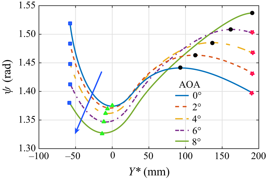
Figure 6. Variations of the relative angle ( $\psi$) along the half part of the lifting body for various angles of attack (AOA) (arrow line denoting the increasing direction). Symbols denote the local extremum points that are associated with certain flow regions, i.e. squares indicate the locations of the windward vortex, triangles the locations of the shoulder attachment line, circles the locations of the shoulder vortex and flowers the leeward attachment line.

Figure 7. ( $a$) The shoulder vortex illustrated by the axial velocity contour at $X^* = 900$ mm, with the up and down edges of the vortex being marked. ( $b$) Comparison of the location of the local maximum of the relative angle ( $\psi _{{max}}$) and the shoulder vortex location bounded by the up and down edges.
3.2. Transitional flow pattern
Figure 8 presents an overview of the transitional flow pattern. The transition regions are shown clearly by the distribution of skin friction coefficient,  $C_f\equiv |2\mu \boldsymbol {\nabla } \bar U|_{{w}}/R$, in figure 8(a,b). The windward vortex region is the first to experience the transition, at $X^* = 1100$ mm, followed by the shoulder vortex region, the windward cross-flow region, and finally the shoulder cross-flow region. Figure 8( $c$) illustrates the transition process of the shoulder vortex. The vortical structures are illustrated using the $Q$-criterion (Hunt, Wary & Moin Reference Hunt, Wary and Moin1988). It can be seen that disturbances first set in the head of the vortex, manifesting as crescent-shaped vortices, and rapidly develop into hairpin packets, contaminating the whole bulge. Figure 8( $d$) displays the evolution of vortical structures in the shoulder cross-flow region. The vortices initially manifest as oblique rolls with angles relative to the azimuthal direction ranging from 30 $^\circ$ to 40 $^\circ$. The spacings of these oblique rolls are nearly twice the boundary layer thickness, and the phase velocities (based on the disturbances of the dominant frequency) are around 0.8, indicating that they probably originate in Mack instability. Moreover, these oblique rolls exhibit prominent azimuthal variations as marked by the red longitudinal bands. These longitudinal bands form an angle of approximately 80 $^\circ$ with respect to the azimuthal direction. Since time-averaged $C_f$ distributions do not show any visible streaks, or footprints of stationary cross-flow vortices, these longitudinal bands likely arise from travelling cross-flow waves. In the locations of the longitudinal bands, $\varLambda$ vortices gradually emerge riding on the oblique rolls, which further develop into hairpin packets and merge with lateral vortices to form a triangle-shaped transition region. Figure 8( $e$) shows the transitional flow pattern in the windward cross-flow region. A triangle-shaped transition region also appears, surrounded by longitudinal streaks with angles of around 70–80 $^\circ$. These longitudinal streaks are again likely associated with travelling cross-flow waves, which is apparent from the supplementary movie of the cross-section flow (available at https://doi.org/10.1017/jfm.2021.1125). Small-scale rolls are observed to ride on the longitudinal streaks, which are believed to develop from secondary instabilities of the travelling cross-flow waves. These rolls would further evolve into hairpin vortices. Note that a similar transition pattern has been observed by Tufts et al. (Reference Tufts, Borg, Bisek and Kimmel2020) in numerical simulations of the boundary layer transition on the HIFiRE-5 elliptic cone where the predominance of the travelling cross-flow waves is also highlighted.
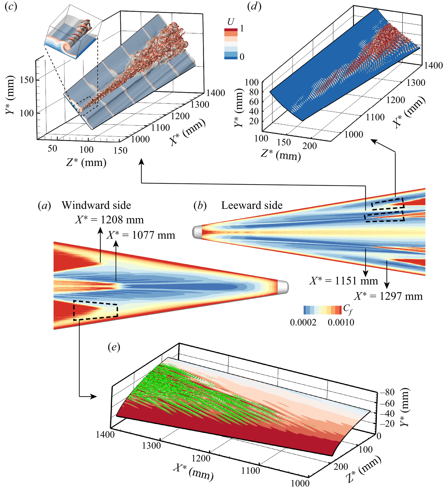
Figure 8. An overview of boundary layer transition on the HyTRV model. ( $a$) Time-averaged skin friction coefficient distribution on the windward side. ( $b$) Time-averaged skin friction coefficient distribution on the leeward side. ( $c$) Instantaneous vortical structures in the shoulder vortex region visualized by the isosurface of the $Q$-criterion ( $Q=0.001$) coloured by the axial velocity, and the isosurface of the axial velocity ( $U = 0.7$), with some velocity slices also displayed. ( $d$) Instantaneous vortical structures (same settings as panel ( $c$)) in the shoulder cross-flow region. ( $e$) Instantaneous flow pattern in the windward cross-flow region, depicted by a wall-normal slice (at the 50th grid point from the wall) coloured by axial velocity, along with the corresponding vortical structures ( $Q=0.001$) coloured by $Q$. The transition locations of different regions are also marked, which are defined where the time-averaged skin friction coefficient reaches 50 % of its maximum value in the late-transition stage along a constant azimuthal-angle ray. Note that the coarse-grid part of the model has been replaced by the mirror region of the fine-grid part.
3.3. Shoulder vortex region
Figures 3 and 8( $c$) illustrate the progression from formation to breakdown of the vortex. A typical flow profile is displayed in figure 7( $a$), depicting a ‘flat-top’-shaped structure. Interestingly, it looks very similar to the boundary layer modulated by low-azimuthal-wavenumber cross-flow vortices on a yawed cone as studied by Moyes et al. (Reference Moyes, Paredes, Kocian and Reed2017b), and (one-half of) the centreline mushroom structure in BoLT as studied by Knutson et al. (Reference Knutson, Thome and Candler2019). To help to determine if the vortex is conducive to inviscid instability, an inflection point calculation was completed. The $\phi$-direction and wall-normal gradients at $X^* = 872$ mm are shown in figure 9, where figure 9(a) would depict the outer mode instability, concentrating on the top shear layer, and figure 9(b) would depict the inner mode instability, residing in the inner shear layer.
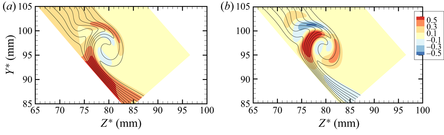
Figure 9. Eight isolines (solid black) of axial velocity  $U$ (from 0.1 to 0.8) and isocontours at $X^* = 872$ mm of normalized gradients ( $a$)
$a$)  $\rho \,\partial U/\partial \delta$ and ( $b$)
$b$)  $\rho \,\partial U/\partial \phi$.
Figure 10 shows the BiGlobal instability results at multiple axial locations along the vortex path from  $X^* = 534$ mm to $X^* = 1000$ mm. At the first station, the Mack mode peaks at around 65 kHz and is the most unstable. In comparison, a shear-layer mode, denoted as mode 1, emerges in a slightly lower-frequency region. The Mack mode resides in the flat body part, whereas mode 1 concentrates on the head part, in accord with the observation by Moyes et al. (Reference Moyes, Paredes, Kocian and Reed2017b) for secondary instabilities of cross-flow vortices with similar shape. An important distinction between the Mack mode and the shear-layer mode corresponds to the wall-normal distribution of the temperature fluctuations. Whereas the Mack mode induces significant fluctuations near the wall, the fluctuations associated with the shear-layer mode are localized within the shear layer in the vicinity of the boundary layer edge. As the vortex develops, the Mack mode decreases in frequency with the increasing boundary layer thickness, and eventually disappears before $X^*=872$ mm. In comparison, mode 1 shifts towards higher-frequency regions and is substantially destabilized. Multiple shear-layer modes denoted by mode 2 to mode 5 also emerge in the meantime. Modes 1–3 cover a broader frequency band, $f^*\in (0,200)$ kHz, in the spectra and possess much higher phase velocities, $c\in (0.7,0.8)$, than modes 4 and 5, which have frequencies below 40 kHz and phase velocities from 0.3 to 0.55.

Figure 10. Variations of growth rates and phase velocities of unstable modes for the shoulder vortex at four axial locations: (a,b)  $X^* = 534$ mm, (c,d) $X^* = 630$ mm, (e,f) $X^* = 872$ mm, and (g,h) $X^* = 1000$ mm. The real parts of the temperature eigenfunctions for the most unstable Mack mode (66 kHz) and mode 1 (50 kHz) are shown at the first station, along with the base flow depicted by the axial velocity (isolines).
The typical mode structure for each shear-layer instability is displayed in figure 11. As expected, all these modes are localized in regions of high shear. In particular, modes 1–3 locate at the outer shear layer and can be referred to as outer modes, whereas the other two modes concentrate on the inner shear layer and can be classified as inner modes. Coexistence of the inner and outer shear-layer modes has also been identified in stability analyses for leeward streamwise vortices of a yawed cone (Chen et al. Reference Chen, Chen, Dong, Xu and Yuan2020; Li et al. Reference Li, Chen, Huang, Yang and Xu2020b) and for centreline streamwise vortices of an elliptic cone (Li et al. Reference Li, Zhang, Liu, Huang, Luo and Zhang2018) and the BoLT model (Li et al. Reference Li, Choudhari and Paredes2020a).

Figure 11. Temperature disturbance structures associated with the locally most unstable disturbance frequency of each mode: ( $a$) mode 1, $f^* = 90$ kHz; ( $b$) mode 2, $f^* = 70$ kHz; ( $c$) mode 3, $f^* = 60$ kHz; ( $d$) mode 4, $f^* = 10$ kHz; ( $e$) mode 5, $f^* = 18$ kHz. Axial velocity isosurfaces ( $U$) are displayed with values of 0.7 for ( $a$–
$a$– $c$) and 0.4 for (d) and (e). The normalized temperature eigenfunction is also shown with the velocity base flow contour in the start slice in (d) and (e).
Next, we adopt PSE3D to trace the evolution of single-frequency disturbances. The  $N$-factors (i.e. the logarithmic amplification ratios relative to the neutral station) of outer modes for a range of frequencies (40,130) kHz are shown in figure 12( $a$). The inner modes are found to be substantially less unstable than the outer modes, thus the results are not displayed here. It can be seen that the component of 70 kHz is dominant until $X^* = 1000$ mm, beyond which the component of 90 kHz achieves slightly larger $N$-factors. The maximal $N$-factor is around 12 near the transition point, slightly smaller than the transition $N$-factor (about 15) for the centreline streamwise vortices of the HIFiRE-5 vehicle at a flight condition (Choudhari et al. Reference Choudhari, Li and Paredes2020). The temperature isosurface of this frequency is shown in figure 12( $b$), which highlights how the regular modal structure stretches to form the crescent-shaped structure in the late stage. The structure pattern closely resembles that of QDNS results preceding transition in figure 8( $c$), indicating that the outer-mode instability is indeed dominant in the transition process. The Mack-mode perturbation (not shown here) undergoes only a short-distance moderate amplification, hence it is unlikely to trigger the breakdown of the vortex.

Figure 12. Downstream evolution of disturbances predicted by PSE3D: ( $a$)
$a$)  $N$-factors for a range of frequencies of (50,130) kHz with step 10 kHz, the thick redline representing 70 kHz; ( $b$) spatial structure of frequency 70 kHz, illustrated by the isosurface of the real parts of temperature disturbances. The isosurface value is prescribed to be 200 times the initial value (i.e. $N = 5.3$). The base flow is also visualized by isosurface $U=0.7$ and contours ( $U$) at several axial stations.
Figure 13 further displays root mean square (r.m.s.) distributions of disturbances and the corresponding spectra at the peak r.m.s. locations for several axial stations. At the first station, fluctuations concentrate on the inner high-shear layer. The peak frequency is around 3 kHz, which is far below the peak inner-mode instability frequency (around 10 kHz) from BiGlobal analysis. One possible explanation for the appearance of such low-frequency disturbances is the non-normal instability mechanism (Schmid Reference Schmid2007) by which very-low-frequency disturbances may attain a rapid growth. Although these low-frequency disturbances can amplify and reach a large amplitude downstream, the low-frequency spectrum seems not to expand and the inner shear layer is not as remarkably distorted as the outer shear layer, indicating that they are unlikely to be the essential factors inducing transition. On the other hand, high-frequency disturbances centred at approximately 70 kHz manifest themselves in the outer shear layer since  $X^*=900$ mm, and quickly become dominant components in the r.m.s. distribution before $X^*=1000$ mm. At the last station, the spectrum in the outer shear layer has been broadened rapidly, indicating the onset of turbulence there. In comparison, a weak peak at around 20 kHz, likely originating in inner-mode instabilities, appears in the spectrum of the sampling point in the inner shear layer. The amplitude evolution of the 70 kHz component is shown in figure 14, clearly depicting the exponential growth and the subsequent saturation stages. Unless otherwise stated, the amplitude of the QDNS results is defined as the maximal value of the temperature fluctuations in the cross-sections. Good agreement between QDNS and PSE3D results initiated by mode 1 can be observed, which is a verification of both approaches. The QDNS values depart from the PSE3D results for $X^*>900$ mm, most likely due to nonlinear modulations, which are known to tend to stabilize the shear-layer instabilities as well as decrease the peak mode frequency (Chen et al. Reference Chen, Huang and Lee2019b, Reference Chen, Chen, Dong, Xu and Yuan2020; Li et al. Reference Li, Chen, Huang, Yang and Xu2020b). Indeed, PSE3D results based on the time-averaged basic states of the transitional flow, which take the nonlinear modulations into account, show a better agreement with QDNS results, as shown in figure 14. The BiGlobal result from integration of growth rates of mode 1 is also displayed. The growth rate predicted by BiGlobal is notably larger than those of PSE3D and QDNS. Such a discrepancy is likely because of non-parallel effects.

Figure 13. Normalized disturbance root-mean-square (r.m.s.) distribution from QDNS at four presentative stations: ( $a$)
$a$)  $X^*= 800$ mm, ( $c$)
$c$)  $X^*= 900$ mm, ( $e$)
$e$)  $X^*= 1000$ mm, and ( $g$)
$g$)  $X^* = 1100$ mm, along with isolines of the time-averaged axial velocity $U$ (from 0.1 to 0.8). The sampling points are marked by filled symbols, and the corresponding spectra are displayed in the right-hand column (b,d, f,h).

Figure 14. Comparison of amplitude evolutions of disturbances with frequency 70 kHz from QDNS and theoretical predictions. The initial amplitudes of PSE3D and BiGlobal are prescribed to be equal to that of PSE3D at  $X^* = 700$ mm.
3.4. Shoulder cross-flow region
Low-frequency cross-flow instabilities and high-frequency Mack instabilities can coexist in the shoulder cross-flow region. Figure 15(a,b) displays the eigenvalue spectra of Mack modes at  $X^* = 1000$ mm from BiGlobal. Multiple Mack modes are present, of which the six most unstable ones are shown. For the sake of clarity, we denote these modes as modes 1–6, with an ordering of ascending phase velocities at frequency 125 kHz. Interestingly, the spacings in the phase velocity between adjacent modes are almost the same for all the modes and remain nearly unchanged with varying frequency. Moreover, phase velocities decrease almost linearly with increasing frequency. From mode 1 to mode 6, the peak growth rate decreases; the left-hand part of the spectrum along with the peak frequency moves towards the high-frequency region, while the right-hand part changes only slightly. Figures 15( $c$–
$c$– $f$) show the real part of the temperature eigenfunction of the first four modes at their peak frequencies. For the purpose of highlighting the spatial scale of the mode, the arc length, $S^*$, starting from the left azimuthal boundary of the BiGlobal computation region, is introduced. A dual-peak structure across the boundary layer can be seen clearly for all the modes, as a prominent feature of Mack-mode instabilities. From mode 1 to mode 4, the azimuthal oscillation appears to be more compact. It is convenient to further divide the boundary layer into three subregions, i.e. the expanding region in the left side connecting to the shoulder vortex region, the contracted region in the right side adjacent to the side attachment-line region, and in between the plateau region where the boundary layer changes slowly. Then one immediately finds that all the modes concentrate mainly in the plateau region, which is probably due to the sensitivity of Mack-mode instability to the azimuthal variations of the boundary layer thickness (Mack Reference Mack1984). This feature also holds for other frequencies. In the research of the HIFiRE-5 elliptic cone by Paredes et al. (Reference Paredes, Gosse, Theofilis and Kimmel2016), Mack modes are found to be the extension of attachment-line instabilities, and their frequencies and growth rates decrease as the location of the mode shape peak moves from the vicinity of the attachment line towards the centreline. In our study, however, Mack modes in the shoulder cross-flow region appear to have no connection with the attachment-line instabilities, since their mode shapes reside only in the plateau region.

Figure 15. Spectra of Mack mode instabilities from BiGlobal calculations at  $X^* = 1000$ mm for the shoulder cross-flow region: ( $a$) spatial growth rates and ( $b$) phase velocities as a function of frequency, and normalized temperature disturbance (real part) distribution in the wall-normal distance ( $\delta ^*$)–arc length ( $S^*$) plane for the most unstable component of mode 1 ( $c$), mode 2 ( $d$), mode 3 ( $e$) and mode 4 ( $f$), at $X^* = 1000$ mm. The position of $S^*=0$ corresponds to the left azimuthal boundary of the computation region in BiGlobal. The temperature base flow (black lines) is also plotted with contour level increments in intervals of 0.5.
Another interesting observation is that all the modes are essentially 3-D or oblique. The obliqueness can be illustrated clearly by the spatial structures of these modes at frequency 128 kHz (which is close to the peak frequency of each mode), as shown in figure 16. The mode structures manifest as two-layer oblique rolls with certain phase lags. Because the upper-layer roll is dominant, the wave angle is estimated from the upper-layer roll. From mode 1 to mode 4, the wave angle decreases from 35 $^\circ$ for mode 1 to 24 $^\circ$ for mode 3 and then increases to 28 $^\circ$ for mode 4. Moreover, the mode with the lower phase velocity tends to reside in locations slightly closer to the shoulder attachment line. Figure 17 further compares spatial structures of mode 1 for three frequencies. The wave angle increases from 20 $^\circ$ at frequency 115 kHz to 37 $^\circ$ at frequency 135 kHz. Since the phase velocity also decreases with increasing frequency, the wave angle of the single mode is also negatively correlated with the mode phase velocity. The azimuthal locations of mode shapes appear to be directly associated with the phase velocity too, as they gradually shift towards the attachment line with decreasing phase velocity. This observation holds qualitatively for other modes.

Figure 16. Spatial structures of the most amplified component for four modes at frequency 128 kHz: ( $a$) mode 1, ( $b$) mode 2, ( $c$) mode 3 and ( $d$) mode 4.

Figure 17. Spatial structures of mode 1 at three frequencies: ( $a$) 115 kHz, ( $b$) 125 kHz and ( $c$) 135 kHz.
Figure 18 displays downstream evolutions of the first three modes with frequency 125 kHz. It can be observed that the growth rates are close between modes and exhibit a parabolic shape peaking at  $X^*\approx 1030$ mm. Moreover, the phase velocities all decrease monotonically along the axial direction. The PSE3D results initiated by mode 1 are also shown for comparison. The growth rate from PSE3D shows a shape similar to that for the BiGlobal results, but it is notably larger than the latter especially for the right-hand half of the parabolic shape. As a result, the amplification region from PSE3D extends almost 50 mm downstream of the neutral location predicted by BiGlobal. The phase velocity from PSE3D decreases more slowly, and its trace crosses the phase velocities of all three modes. This suggests that the disturbances in PSE3D would excite multiple modes due to non-parallel effects when they travel downstream, and behave as a combination of multiple modes rather than as a single mode.

Figure 18. Downstream evolutions of the first three Mack modes with frequency 125 kHz: ( $a$) growth rates and ( $b$) phase velocities. The PSE3D results initiated by mode 1 are shown for comparison.
The spatial structures of mode 1 from BiGlobal are depicted in figure 19 for three representative axial locations. Obviously, in the axial direction, the wave angle increases and the mode structures move towards the shoulder attachment line, again implying a strong correlation with phase velocity (recall that the phase velocity also decreases along the axial direction).

Figure 19. Spatial structures of mode 1 with frequency 125 kHz at three axial locations: ( $a$)
$a$)  $X^* = 952$ mm, ( $b$)
$b$)  $X^* = 1048$ mm and ( $c$)
$c$)  $X^* = 1144$ mm.
Downstream evolution of the Mack-mode instability for various frequencies by PSE3D are further illustrated in figure 20. Note that various inlet modes will lead to various evolution routes, and the most amplified one of each frequency is shown in figure 20( $a$). The dominant frequency decreases with increasing axial locations, in accord with the growth of boundary layer thickness. The largest $N$-factor is approximately 4.5 at $X^* = 1250$ mm by frequency 125 kHz. The corresponding mode shapes at four axial stations, along with the base flow, are displayed in figures 20( $b$–
$b$– $e$). The azimuthal wavelength ( $\lambda_\phi$ defined as the width between adjacent peaks of the mode shape) remarkably decreases from around 20 mm at the first slice to nearly 10 mm at the last slice, resulting in increases of the wave angle. This is consistent with the decrease of the phase velocity as shown in figure 18( $b$). As the Mack-mode wave travels downstream, the main part of the mode structure remains in nearly the same range of the azimuthal angles (i.e. $\phi \in (74,83)^\circ$), rather than moving towards the shoulder attachment line as implied by BiGlobal.

Figure 20. The PSE3D results for Mack-mode disturbances. Downstream evolution of  $N$-factors of representative frequencies ( $a$). Distribution of disturbance of 125 kHz at four axial stations: ( $b$)
$b$)  $X^* = 945$ mm, ( $c$)
$c$)  $X^* = 1017$ mm, ( $d$)
$d$)  $X^* = 1100$ mm and ( $e$)
$e$)  $X^* = 1185$ mm, illustrated by contours of the real part of the normalized temperature fluctuations, along with the temperature base flow.
The cross-flow instabilities are caused by the inflectional three-dimensional boundary layer profile formed over the surface of the leeward zone between the shoulder attachment line and the shoulder vortex. Therefore, their shape functions are expected to occupy a much wider region in the azimuthal direction than the Mack-mode instabilities do. As a result, large resolutions are required to solve these modes using the BiGlobal analysis. Numerical tests show that cross-flow instabilities are relatively insensitive to the wall-normal resolution. Hence we fixed the wall-normal grids number  $N_\delta$ to 101 and vary the azimuthal grids number $N_\phi$ from 160 to 2000. It turns out that the eigenvalues undergo an overall decrease in growth rate with increasing azimuthal resolution, but they do not converge, as shown in Appendix C. This implies that the eigenvalue problem for the cross-flow instabilities are extremely sensitive to the numerical fluctuations that likely arise from truncation and interpolation errors (Trefethen & Embree Reference Trefethen and Embree2005). Paredes et al. (Reference Paredes, Gosse, Theofilis and Kimmel2016) seemed to have also noted the bad convergence of this eigenvalue problem, but they did not show the spectra so we cannot make a comparison.
Now we consider the mode shape of a typical cross-flow mode with frequency 20 kHz as shown in figure 21. It can be seen clearly that the cross-flow mode exhibits a wave packet distribution with the oscillation amplitude vanishing towards the azimuthal boundaries. The negligibly small values in the vicinity of the azimuthal boundaries indicate that the cross-flow instability is insensitive to the azimuthal boundary conditions. The rapid oscillation of the mode shape translates into a small azimuthal wavelength and a large wave angle. In contrast, the envelope of the mode shape is much smoother. Furthermore, the azimuthal wavelength changes little along the azimuthal direction. Therefore, we can seek a Wentzel–Kramers–Brillouin–Jeffrey-like expansion (Bender & Orszag Reference Bender and Orszag1978) of the mode shape as
 \begin{equation} \hat{\boldsymbol q}(\delta,\phi) = \tilde{\boldsymbol q}(\delta,\phi)\exp({\rm i}4{\rm \pi}\beta \tilde S), \end{equation}
where  $\tilde S \in [0,1]$ is the normalized form of the arc length $S^*$, so that the rapid variations are absorbed into the exponential term (much akin to the PSE methodology). As a result, the equation (2.9) reduces to
 \begin{equation} \left(\begin{array}{cc} \boldsymbol{0} & \boldsymbol{I} \\ -\tilde{\boldsymbol A_0} & -\tilde{\boldsymbol A_1} \end{array}\right) \left(\begin{array}{c} \tilde{\boldsymbol q} \\ \alpha \tilde{\boldsymbol q} \end{array}\right) = \\ \alpha \left(\begin{array}{cc} \boldsymbol{I} & \boldsymbol{0} \\ \boldsymbol{0} & \tilde{\boldsymbol A_2} \end{array}\right) \left(\begin{array}{c} \tilde{\boldsymbol q} \\ \alpha \tilde{\boldsymbol q} \end{array}\right), \end{equation}
where the azimuthal wave number  $\beta$ has been included in the modulated linear operators with a tilde ( $\,\tilde{}\,$) over it. It should be noted that the reduced eigenvalue equation (3.3) is completely equivalent to the original one (2.9) since no additional assumptions have been introduced. Similarly, this methodology can be applied straightforwardly to PSE3D with a fixed $\beta$ along the axial direction.

Figure 21. Comparison of results from the conventional eigenvalue problem with 1000 azimuthal grid points and the reduced eigenvalue problem with 160 azimuthal grid points for a typical cross-flow mode with frequency 20 kHz. ( $a$) Temperature disturbance illustrated by its real part (filled contours from (2.9)) and by its amplitude function (contour lines from (3.3)); ( $b$) wall pressure disturbance illustrated by its real part (blue line from (2.9)) and by its amplitude function (red line from (3.3)).
In calculation, we can choose an appropriate wavenumber  $\beta$, which can be a constant or can vary slowly with $\phi$, in order to make the amplitude term, $\tilde {\boldsymbol q}(\delta,\phi )$, a slowly varying function of $\phi$. As a benefit, the azimuthal grid points required to obtain a smooth solution can be largely reduced.
Figure 22 shows the convergence test of the reduced eigenvalue problem for 20 kHz. For  $N_\phi \ge 240$, the eigenvalues concentrate in a parabolic-like band but exhibit small shifts with increasing azimuthal grid points. The magnitudes of such shifts do not show a decreasing trend with increasing resolution, indicating that the reduced eigenvalue problem can hardly converge too. Nevertheless, the eigenvalue fluctuations with increasing resolution are much smaller than those obtained from the conventional equation (2.9) with the same grid points, as shown in figure 46. It is noteworthy that varying $\beta$ in a certain range, which acts as perturbations to the eigenvalue equation, would lead to shifts of the eigenvalues in a manner similar to changing grid resolution, as shown in Appendix D. Figure 22( $b$) compares the fluctuation amplitude distribution of the mode calculated from three resolutions as marked by the ellipse in figure 22( $a$). As expected, the small eigenvalue shift between two resolutions corresponds to a small shift of the mode shape distribution. Unless otherwise stated, the azimuthal grid points used in multi-dimensional stability calculations for the cross-flow instability are 240 hereafter.

Figure 22. Convergence test for the cross-flow instability (20 kHz) with varying azimuthal resolutions: ( $a$) spectra at $X^* = 1000$ mm; ( $b$) contours of the amplitude term magnitudes, $|\hat q|$ for the modes enclosed by the ellipse curve in ( $a$), along with the temperature base flow. The chosen wavenumber $\beta$ is prescribed to be an integer and decreases linearly from 26 to 8 as the phase velocity increases.
Spectra variations with frequency at  $X^*=1000$ mm are displayed in figure 23. It can be observed that the travelling cross-flow instability is more unstable than the stationary counterpart, and the maximum growth rate occurs at approximately 35 kHz; the phase velocity, ranging from 0.2 to 0.6, increases with frequency, which agrees with the experimental results obtained by Borg et al. (Reference Borg, Kimmel, Hofferth, Bowersox and Mai2015) for the HIFiRE-5 elliptic cone.

Figure 23. Spectra for the cross-flow instability with various frequencies at  $X^* = 1000$ mm: (a) spectra in the $-\alpha _i^*$– $c$ plane, (b) spectra in the $c$–
$c$– $f^*$ plane.
Now we consider the spatial structures of the cross-flow instability. Figure 24 shows the real part of the shape function,  $\hat q(\delta,\phi )$, for three modes with the same frequency (20 kHz) but different phase velocities, highlighting the streaky structures arising from the crossflow modes. The shape function (and all such terms hereafter) is recovered by first interpolating the amplitude term onto a finer grid and then multiplying by the phase term, ${\rm e}^{4\,{\rm i}{\rm \pi} \beta \tilde S}$. With increasing phase velocity, the shape function moves towards the shoulder vortex region with larger azimuthal wavelengths. The wave angles of the streaks are estimated to be around 80 $^\circ$. With increasing frequency the opposite trend is seen on the modal structure, as shown in figure 25, although the phase velocity also increases. This indicates that the frequency is a more important factor than the phase velocity in determining the behaviour of the modal structure.

Figure 24. Isosurfaces of the normalized real part of the temperature eigenfunction ( $\hat T_r = 0.5$) for three modes with the same frequency 20 kHz: ( $a$)
$a$)  $c = 0.27$, $\beta = 23$,( $b$)
$b$)  $c=0.35$, $\beta = 16$ and ( $c$)
$c$)  $c = 0.43$, $\beta = 10$. Twice the axial wavelength of each mode is shown.

Figure 25. Isosurfaces of the normalized real part of the temperature eigenfunction ( $\hat T_r = 0.5$) for the most amplified mode of three frequencies: ( $a$)
$a$)  $f^* = 10$ kHz, $c = 0.23$, $\beta = 15$, ( $b$)
$b$)  $f^* = 25$ kHz, $c=0.37$, $\beta = 18$ and ( $c$)
$c$)  $f^* = 45$ kHz, $c = 0.49$, $\beta = 20$. Twice the axial wavelength of each mode is shown.
Next we examine how the cross-flow instability changes with axial locations. Without loss of generality, take the modes of 20 kHz, for example. The spectra at three stations, i.e.  $X^* = 800$ mm, 1000 mm and 1200 mm, are shown in figure 26 along with the shape function of the most unstable mode at each station. The cross-flow instability is seen to be enhanced from $X^* = 800$ mm to 1200 mm, whereas the phase velocity of the dominant mode changes little. It is evident from figure 26( $b$–
$b$– $d$) that the dominant mode moves towards the shoulder attachment line.

Figure 26. Spectrum variation with axial locations ( $\square$ $X^* = 800$ mm, $\triangle$ $X^* = 1000$ mm, $\bigcirc$ $X^* = 1200$ mm) for the cross-flow instability of 20 kHz. The real part of the temperature shape function of the most unstable mode at each station (marked by the circle) is displayed in ( $b$–
$b$– $d$).
$d$).
However, because the eigenvalue spacing is very small, disturbances will always be composed of multiple modes rather than being dominated inevitably by any single mode as they travel downstream. As a result, accurately tracking a single mode in the axial direction is nearly impossible and also of insignificance in practice. In comparison, PSE3D is able to capture adequately evolution of instabilities in the context of multiple modes (Chen et al. Reference Chen, Chen, Yuan, Tu and Zhang2019a; Choudhari et al. Reference Choudhari, Li and Paredes2020), and turns out to be less sensitive to the grid resolution, as shown in Appendix E. Therefore, we utilize PSE3D to follow evolutions of cross-flow instabilities in this paper. Figure 27(a,b) show the evolution of  $N$-factors and phase velocities obtained by PSE3D with frequency 30 kHz but different initial conditions, say different inlet modes or different inlet locations. It is obvious that various initial conditions lead to different routes. Hence it is necessary to seek the optimal initial condition that produces the largest $N$-factor at the outlet in order to estimate the transition criterion. Principally, the optimal disturbances can be determined by solving iteratively the PSE3D and its adjoint counterpart just as in the one-dimensional case (see, for example, Paredes et al. Reference Paredes, Gosse, Theofilis and Kimmel2016), which is, however, beyond the scope of this work. Another important observation is that the phase velocities of all the routes substantially increase in the axial direction, whereas the BiGlobal analysis shows that the most unstable mode remains at nearly the same phase velocity along the axial direction. Figure 27(c,d) further compare the most amplified route of four frequencies. One can observe that the dominant frequency is 30 kHz for $X^*<1200$ mm and changes to 40 kHz before the outlet. The largest $N$-factor near the transition location (1297 mm) is slightly above 5.

Figure 27. The PSE3D results for the cross-flow instability of 30 kHz with various initial conditions (a,b) and of the most amplified one for each frequency (c,d). The most amplified route of 30 kHz is denoted by the thick line. (a,c)  $N$-factor, (b,d) phase velocities.
Figure 28 illustrates the real parts of the temperature shape functions at five successive axial stations for the most amplified route of frequency 20 kHz. For routes with higher (lower) initial phase velocity, the shape functions would exhibit a larger (smaller) azimuthal wavelength and lie closer to (farther away from) the shoulder vortex region. In this case, the main part of the shape functions from PSE3D remains in the plateau region, rather than moving towards the attachment line as indicated by the BiGlobal results above. The distribution of fluctuations of 20 kHz from QDNS are also shown for comparison. Clearly, regular cross-flow wave profiles also appear and reside almost exclusively in the plateau region. After the fourth station,  $X^* = 1100$ mm, the cross-flow wave profile is obviously distorted in a manner such that its left-hand part is notably enhanced and substantially stretched in the wall-normal direction. Such distortion is likely caused by nonlinear interactions with the Mack-mode instability. Furthermore, the azimuthal wavelength ( $\approx 6$ mm) is slightly larger than the PSE3D results ( $\approx 5$ mm) and also does not exhibit any prominent variations along the axial direction.

Figure 28. Comparison of evolution for the real parts of the normalized temperature disturbances from PSE3D results (left column) initiated by modes with phase velocity  $c=0.37$ and QDNS results (right column) at five successive stations: $X^* = 800$ mm, 900 mm, 1000 mm, 1100 mm and 1200 mm. The disturbance frequency is fixed at 20 kHz.
A more realistic disturbance pattern can be obtained by taking the amplitude growth into account. Figure 29 shows the spatial evolution for the travelling cross-flow wave with frequency 20 kHz and for the Mack-mode wave with frequency 125 kHz, using isosurfaces at a value of 10 times the initial amplitude. Whereas the cross-flow wave first enters the exponential growth phase, the Mack-mode wave undergoes a faster growth so that both types of instability start to manifest themselves at nearly the same axial location. The cross-flow waves form longitudinal streaks with wave angles of around 84 $^\circ$, while the Mack-mode wave appears as oblique rolls with a wave angle of 30–40 $^\circ$. Because PSE3D marching stops at the neutral point where the growth rate of disturbance becomes negative, Mack-mode structures are invisible far downstream. Downstream increase of the magnitude leads to a triangle-shaped pattern for both kinds of instability. The overlap of the distribution regions indicates possible interactions between two kinds of instabilities, as has been observed in inclined hypersonic cone boundary layers (Munoz, Heitmann & Radespiel Reference Munoz, Heitmann and Radespiel2014; Dong et al. Reference Dong, Chen, Yuan, Chen and Xu2020). Inviscid streamlines are also displayed in figure 29. The relative angles of the travelling cross-flow wavefronts and the Mack-mode wavefronts with respect to the edge streamlines are estimated to be approximately 11 $^\circ$ and 58 $^\circ$, respectively.

Figure 29. The structure evolution, illustrated by the real part of the temperature disturbance, for the cross-flow instability with frequency 20 kHz (the black isosurface) and the Mack-mode instability with frequency 125 kHz (the red isosurface). The isosurface value is prescribed to be 10 times the initial value (i.e.  $N = 2.3$). The edge streamlines are also shown (blue lines) for reference.
Figure 30 shows the fluctuation distributions from QDNS for three axial stations. The disturbance spectra are evaluated at locations where the r.m.s. amplitude is at its peak. The spectrum at the first station exhibits a prominent low-frequency peak at approximately 23 kHz and a much weaker high-frequency peak at approximately 190 kHz. The low-frequency peak corresponds to the travelling cross-flow instability, while the high-frequency peak emerges from the Mack-mode instability, as shown by the above analyses. Further downstream, at  $X^* = 1000$ mm, a dual-peak r.m.s. amplitude structure is manifest in the plateau region. The fluctuation amplitude in the upper layer is larger and displays two isolated peaks. The spectra indicate that the Mack-mode wave amplitude appears to be larger in the left peak, while the travelling cross-flow instability dominates in the right peak. This is consistent with the distribution feature of these two kinds of instabilities. The Mack-mode fluctuations prevail at the last station. The appearance of its first harmonic implies that self-interactions are present. Owing to the increase of the boundary layer thickness, the Mack-mode instability decreases in frequency as it travels downstream.

Figure 30. Normalized disturbance r.m.s. amplitude distribution from QDNS at three representative stations: ( $a$)
$a$)  $X^* = 800$ mm, ( $c$)
$c$)  $X^* = 1000$ mm and ( $e$)
$e$)  $X^* = 1200$ mm, along with the temperature base flow. The sampling points are marked by filled circles, and the corresponding spectra are displayed in ( $b$), ( $d$) and ( $\,f$).
Figure 31 compares the amplitude evolutions of Mack-mode waves with frequency 125 kHz and cross-flow waves with frequency 20 kHz from QDNS and PSE3D results. The QDNS results indicate that the Mack-mode wave starts to amplify after  $X^*=900$ mm and reaches saturation before $X^* = 1200$ mm. The cross-flow wave is observed to grow at least before $X^* = 700$ mm, and becomes saturated after $X^*=1300$ mm. The Mack-mode wave amplitude grows more rapidly and soon reaches the same amplitude level as the cross-flow wave at $X^* = 1100$ mm. The PSE3D results based on the most amplified case can capture adequately the exponential stage of both instabilities, but underestimate the initial growth rates of disturbances. This discrepancy is likely owing to the transient growth of the disturbances in QDNS. Moreover, a notable deviation between QDNS and PSE3D results is observed for the cross-flow wave amplitude for $X^*> 1000$ mm, which is likely attributed to the nonlinear effects from the Mack-mode waves, in accord with the distortion of shape functions as shown in figure 28.

Figure 31. Comparison of axial evolution of amplitudes of the low-frequency cross-flow waves with frequency 20 kHz and the high-frequency Mack-mode waves with frequency 125 kHz from QDNS and PSE3D. The PSE3D results based on the time-averaged profiles of the transitional state are not shown because they are almost indistinguishable from those based on the laminar state in this case.
3.5. Windward cross-flow region
In this subsection, we will consider boundary layer stability in the windward crossflow region. The stability calculations are performed with the same methodology as in the shoulder cross-flow region. The Mack-mode instability is found to be only marginally unstable, i.e. its growth rate is one order of magnitude smaller than the maximal growth rate of the cross-flow instability, hence its stability characteristics will not be discussed further. The cross-flow instability in this region closely resembles that in the shoulder cross-flow region but also exhibits some distinct features. Figure 32 shows the cross-flow instability spectra at  $X^* = 1000$ mm. It is seen clearly that multiple unstable modes are present for each frequency; modes of each frequency occupy a certain band of phase velocity, and the band increases in value but shrinks in width with frequency. The most unstable frequency lies between 15 kHz and 25 kHz, with the maximal growth rate being approximately 15 m $^{-1}$, compared to the case of the shoulder cross-flow region, the peak frequency being lower and the peak growth rate being larger.

Figure 32. Spectra for the cross-flow instability with various frequencies at  $X^* = 1000$ mm in the windward cross-flow region: ( $a$) spectra in the $-\alpha _i^*$– $c$ plane and ( $b$) spectra in the $c$–
$c$– $f^*$ plane.
Next we examine the mode shapes of the cross-flow instability. Figure 33 compares the spatial structures of modes at a fixed frequency with increasing phase velocity. It can be seen that the travelling cross-flow wave lies far away from both the shoulder attachment line and the windward centreline, implying insensitivity to the azimuthal boundary conditions, as is also noted by Lakebrink et al. (Reference Lakebrink, Paredes and Borg2017). The isosurface of the temperature eigenfunction exhibits streaky structures that are inclined towards the windward vortex region. From the attachment line to the windward centreline, the local azimuthal wavelength slightly increases in accord with the growth of the boundary layer thickness, accompanied by a moderate decrease of wave angle. In comparison, the crossflow modal structure in the shoulder crossflow region does not show prominent azimuthal variations because the boundary layer thickness of the shoulder crossflow region possesses a plateau region. Moreover, compared to the crossflow mode of the same frequency in the shoulder crossflow region, the azimuthal wavelength is notably larger and the wave angle is smaller in the case of the windward crossflow region. With increasing phase velocity, the azimuthal wavelength increases and the wave angle decreases, but the spatial location does not change. This trend is somewhat different from the case of the shoulder crossflow region.

Figure 33. Isosurfaces of the normalized real part of the temperature eigenfunction ( $\hat T = 0.5$) for three modes with the same frequency 20 kHz in the windward cross-flow region: ( $a$)
$a$)  $c = 0.4$, $\beta = -18$, ( $b$)
$b$)  $c=0.44$, $\beta = -14$, ( $c$)
$c$)  $c = 0.49$, $\beta = -8$. Twice streamwise wavelengths of each mode are shown. The averaged azimuthal wavelength and the wave angles at two sides are also displayed.
The frequency effects on the mode shape are highlighted in figure 34, showing spatial structures of most unstable modes of three frequencies. With increasing frequency, the azimuthal wavelength decreases and the spatial distribution shifts towards the shoulder attachment line, similar to the case of the shoulder crossflow region. The wave angle also decreases as frequency increases.

Figure 34. Isosurfaces of the normalized real part of the temperature eigenfunction ( $\hat T = 0.5$) for the most unstable modes of three frequencies in the windward crossflow region: ( $a$)
$a$)  $f^* = 5$ kHz, $c = 0.20$, $\beta = -12$, ( $b$)
$b$)  $f^*=20$ kHz, $c = 0.44$, $\beta = -14$, ( $c$)
$c$)  $f^* = 40$ kHz, $c = 0.56$, $\beta = -17$. Twice streamwise wavelengths of each mode are shown. The averaged azimuthal wavelengths and the wave angles at two sides are also displayed.
The downstream evolution of cross-flow instability is studied with PSE3D. Like the case of the shoulder cross-flow region, the  $N$-factor curve (not shown here) is very sensitive to the initial conditions. The maximal $N$-factor value is around 7 preceding the transition point for the frequency range 15–25 kHz. The spatial structure is relatively more robust to the initial conditions and is thus more helpful to characterize the cross-flow mode. Figure 35 shows the spatial evolution of the travelling cross-flow wave with frequency 15 kHz using isosurfaces. As the wave amplitude increases downstream, the number of streaks increases substantially, forming a triangle-shaped spatial distribution. In the direction away from the attachment line, the azimuthal wavelength increases while the wave angle decreases. Take the outlet location, for example: the azimuthal wavelength increases from around 7 mm to 16 mm, while the wave angle decreases from around 82 $^\circ$ to 65 $^\circ$.

Figure 35. The structure evolution from PSE3D for the cross-flow instability with frequency 15 kHz, illustrated by the real part of the temperature disturbance. The isosurface value is prescribed to be 10 times the initial value. The edge streamlines are also shown (blue lines) for reference.
Figure 36 shows the distributions of normalized r.m.s. amplitude of the temperature fluctuations from QDNS for several axial locations. The spectra calculated at the locations where the r.m.s. value is maximum are also displayed. The results indicate that low-frequency components arising from travelling cross-flow waves (peaking at approximately 17 kHz before the last location) dominate the transition process, which is consistent with the stability analyses results. High-frequency disturbances, likely originating in the Mack-mode instabilities, emerge after  $X^* = 1000$ mm and amplify downstream due to the modulation of the cross-flow waves. The onset of turbulence is manifest at the last station, $X^* = 1300$ mm, where the base flow is significantly distorted, and the spectrum is filled up with a scaling law, $|T'|\sim f^{-4}$, describing the behaviour of the temperature fluctuation amplitude in the high-frequency region.

Figure 36. Normalized temperature fluctuation distributions from QDNS at four representative stations: (a)  $X^* = 900$ mm, ( $c$)
$c$)  $X^* = 1000$ mm, ( $e$)
$e$)  $X^* = 1200$ mm and ( $g$)
$g$)  $X^* = 1300$ mm, along with the temperature base flow. The sampling points are marked by $\bullet$ with the corresponding spectra being displayed in the right-hand column. Note that the r.m.s. in the vicinity of the windward centreline has been omitted. A zoom-in plot is displayed in ( $d$) to highlight the high-frequency peak. A log-log plot is added in ( $h$) to indicate the scaling law of the spectrum. The green and black triangles denote the locations of the attachment line and the windward centreline, respectively.
Figure 37 further compares the amplitude evolutions of the travelling cross-flow waves with frequency 15 kHz from QDNS and PSE3D results. Good agreement can be observed except for the initial transient stage and the late nonlinear saturation stage, where the linear amplification seems to be weakened by the mean flow distortion.

Figure 37. Comparison of streamwise amplitude evolutions of the low-frequency cross-flow waves with frequency 15 kHz from QDNS and PSE3D based on either the laminar state or the transitional state.
3.6. shoulder attachment line
The spatial eigenvalue spectrum for the shoulder attachment-line instability from BiGlobal calculations at  $X^* = 1000$ mm is displayed in figure 38. In contrast to previous studies on the attachment-line instability where alternatively arranged symmetrical and antisymmetrical instabilities exist, only one branch of instability is identified in the present case and it no longer possesses perfect spanwise symmetry due to the symmetry breaking of base flow. The peak growth rate is slightly larger than that of the boundary layer instabilities in cross-flow regions, but smaller than that of the shear-layer instabilities in the vortex regions. Because of the small boundary layer thickness ( ${\sim}0.5$ mm here), this instability lies in an extremely high frequency range ( $600\ {\rm kHz} < f^*<700\ {\rm kHz}$), which corresponds to a very small axial wavelength. Such high temporal and spatial oscillations are beyond the present numerical resolution. Therefore, the attachment-line boundary layer remains laminar throughout the whole model in the simulation. The real parts of the normalized temperature eigenfunctions of three representative modes, along with their spatial structures, are shown in figure 39. These eigenfunctions all exhibit dual-peak structures across the boundary layer, which is strong evidence of the Mack-mode instability. The smallest frequency mode resides almost exclusively in the windward side, and behaves like an oblique Mack mode with wave angle approximately $21^\circ$. The middle one, which is also the most amplified one of the branch, is distributed nearly equally in both the windward and leeward sides. Its windward-side part has wave angle approximately $14^\circ$, while its leeward-side part is less oblique, with the opposite wave direction. The largest frequency mode, mainly concentrating in the leeward side, is essentially planar. The attachment-line instability does not extend towards the leeward side as far as it does towards the windward side. This is likely due to the asymmetry of the boundary layer as shown in figure 39( $g$). The boundary layer changes slowly in the vicinity of the $Y^*=0$ plane, but grows fast in both sides. Fast variations of boundary layer in the azimuthal direction likely inhibit the Mack-mode instability, as observed in the shoulder region. Moving away from the $Y^*=0$ plane, the boundary layer thickness in the leeward side increases faster than that does in the windward side, hence the Mack-mode instability is expected to decay faster in the leeward side than in the windward side.

Figure 38. Spatial spectrum of the shoulder attachment-line instability from BiGlobal calculations at  $X^* = 1000$ mm. ( $a$) Spatial growth rate as a function of frequency; ( $b$) phase velocity as a function of frequency.

Figure 39. Real part of the normalized temperature eigenfunction from BiGlobal for three representative modes at  $X^* = 1000$ mm: ( $a$) 615 kHz, ( $b$) 655 kHz, ( $c$) 695 kHz. The corresponding spatial structures, including eight axial wavelengths, are shown in ( $d$–
$d$– $f$), illustrated by isosurfaces of real parts of temperature at value 0.5. The boundary layer in the vicinity of the attachment line is shown in ( $g$).
$g$).
The spatial evolutions of fixed frequency disturbances are evaluated with the help of PSE3D. Figure 40 displays the axial evolutions of  $N$-factors for disturbance frequencies from 610 to 690 kHz. As the streamwise coordinate increases, the boundary layer thickens and the frequency of the Mack mode decreases. The mode with frequency 610 kHz achieves an $N$-factor of 15 near the rear part of the model, which could potentially lead to laminar–turbulent transition (Tu et al. Reference Tu, Wan, Chen, Yuan and Chen2019). Without loss of generality, we consider in detail the spatial structure evolution for the mode $f^* = 650$ kHz, whose $N$-factor first reaches 10. Figure 41( $a$) depicts the whole disturbance structure illustrated by the isosurface of the real part of the temperature component. It can be observed that the attachment-line disturbances first manifest themselves in the windward side. This coincides with the above BiGlobal results since fixed-frequency disturbances tend to be located in the low-frequency part of the unstable branch in the upstream boundary layer, thereby being expected to appear in the windward side. Immediately downstream of their emergence, the attachment-line disturbances quickly form a nearly symmetrical crescent structure, as shown clearly in figure 41( $b$), similar to the structure of the locally dominant mode. The slice in the $X^*$– $Z^*$ plane depicted in figure 41( $c$) also exhibits a dual-peak disturbance structure, as expected. Further downstream, the disturbances gradually move towards the leeward side, as shown in figure 41( $d$). This is again consistent with the BiGlobal results. Another important observation is that the disturbances virtually do not expand in the azimuthal direction as they travel downstream, likely because there is a fast increase of the boundary layer thickness away from the attachment line. This also suggests that the attachment-line instability may not interact with or excite boundary layer instabilities in the outboard region.

Figure 40. Streamwise evolution of  $N$-factors of attachment-line instabilities from PSE3D for various frequencies from 610 kHz to 690 kHz.

Figure 41. Spatial evolution of the attachment-line wave with frequency 650 kHz from PSE3D. ( $a$) The overall structure depicted by the isosurface of the real part of temperature perturbation; the isosurface value is prescribed to be 10 times the initial value. ( $b$) Zoomed-in image of the spatial structure corresponding to the middle squared region in ( $a$). ( $c$) The normalized real part of the temperature disturbance in the $X^*$– $Z^*$ plane marked by the yellow line ( $Y^*=0$). ( $d$) Zoomed-in image of the spatial structure corresponding to the rear squared region in ( $a$), with the isosurface value of 5000 times the initial value to highlight the feature of disturbance distribution.
4. Summary and conclusions
Large-scale numerical simulations using up to 3.1 billion grid points are carried out on boundary layer transitions over the HyTRV geometry lifting body at 2 $^\circ$ angle of attack under a typical Mach 6 wind tunnel condition. The boundary layer is perturbed by random blowing and suction right downstream of the tip to model the transition process. The complex flow configuration leads to a complex pressure distribution over the mode surface, which in turn induces the formation of windward and shoulder vortex regions, shoulder and leeward attachment-line regions, and cross-flow regions in between. A systematic parametric study is then presented on the modal multi-dimensional linear instabilities of the boundary layer over four regions, i.e. the shoulder vortex region, the shoulder cross-flow region, the windward cross-flow region, and the shoulder attachment-line region. The analyses are performed by utilizing spatial BiGlobal, which fully resolves the base flow and its perturbations at selected axial locations on planes normal to the model axis, and by utilizing PSE3D, which tracks the axial evolution of fixed-frequency disturbances. Conclusions are made below for each region considered, and some important data are summarized in table 1.
Table 1. Summary of the transition simulation and stability analysis results for interested regions. The transition  $N$-factor, $N_t$, is defined as the maximum value of the $N$-factor based on PSE3D results at the transition point estimated from the numerical simulation.
In the shoulder vortex region, a ‘flat-top’ asymmetry vortex develops, and is conducive to low-frequency inner shear-layer modes and high-frequency outer shear-layer modes. The outer mode 70 kHz is found to be the most dangerous one leading to the transition. It manifests as crescent-shaped vortices riding on the outer shear layer of the vortex in the linear stage, and evolves into hairpin vortices when nonlinear effects come into play. A Mack mode also exists in the upstream region, but ultimately disappears without transferring to a shear-layer mode as it travels downstream.
In the shoulder cross-flow region coexist high-frequency Mack-mode instabilities and low-frequency cross-flow-mode instabilities. For the Mack-mode instabilities, some important findings are as follows. Multiple Mack modes are present and occupy the same unstable frequency range; these modes are essentially oblique, with wave angles ranging from 20 $^\circ$ to 40 $^\circ$; the Mack-mode waves moving downstream are confined in the plateau region where the azimuthal variations of the boundary layer are mild, and exhibit a decreasing trend in both phase velocities and azimuthal wavelengths. As for the cross-flow modes, their mode shapes oscillate very rapidly and extend over almost the entire surface of the shoulder cross-flow region. By separating the rapidly varying phase term from the slowly varying amplitude term, the required azimuthal grid points are substantially reduced from $O(1000)$ to $O(100)$. However, we note that mode growth rates and phase velocities can hardly converge, suggesting that the eigenvalue problem for the cross-flow instability is highly sensitive to numerical perturbations. Alternatively, the pseudospectra (see, for example, Trefethen & Embree Reference Trefethen and Embree2005) are probably more appropriate to describe the eigenvalue behaviours. Nevertheless, other crucial characteristics, such as eigenfunctions and the spectrum pattern, are robust, so the BiGlobal results can still shed light on the features of cross-flow instabilities. Some important features of cross-flow eigenmodes are uncovered by BiGlobal, as follows.
(1) Travelling cross-flow modes are more unstable than stationary ones.
(2) A great number of modes are present for a single frequency at one axial location.
(3) The phase velocity of the dominant mode increases with increasing frequency, in accord with experimental observations (e.g. Borg et al. Reference Borg, Kimmel, Hofferth, Bowersox and Mai2015).
(4) Increasing the phase velocity tends to increase the azimuthal wavelength and to shift the spatial structure away from the attachment line, whereas an opposite trend is observed by increasing the frequency.
The PSE3D results are also computed to trace the evolution of cross-flow instability disturbances initiated by the BiGlobal solution. With marching downstream along the axial direction, the phase velocity is increased substantially while the azimuthal wavelength changes little, contradicting the trend predicted by BiGlobal. Moreover, PSE3D solutions are sensitive to the initial profiles, but are robust to the grid points. Therefore, one need to perform optimal analyses in order to estimate accurately the transition  $N$-factor. Furthermore, the cross-flow mode and the Mack mode, with comparable integrated amplifications, are found to share an overlap region in spatial distribution, and thereby likely interact with each other. Work is underway to address this issue.
While cross-flow instabilities in the windward cross-flow region are essentially the same as those in the shoulder cross-flow region, some differences lie in specific aspects. For example, the former possess a slightly lower peak frequency, a larger peak growth rate and larger azimuthal wavelengths, as well as smaller wave angles. The crucial difference in stability characteristics between the windward and shoulder cross-flow regions comes from the Mack-mode instability. The Mack mode in the windward cross-flow region is marginally unstable, thereby unlikely to become the dominant primary instability.
Comparisons between theoretical results and numerical results are made when possible. The PSE3D results prove generally to agree well with the QDNS results, especially for the exponential growth stage of instabilities. While the BiGlobal analysis successfully captures the basic features of the instabilities in terms of the peak frequency and the spatial structure, it might fail to predict the axial evolution of disturbances, particularly of the instabilities in cross-flow regions, and exhibits notable discrepancies with QDNS results in terms of growth rates.
Finally, multi-dimensional stability analyses performing on the shoulder attachment line identify only one asymmetry Mack mode, contrary to the common knowledge that multiple unstable modes with alternating symmetry and antisymmetry are present. This suggests that symmetry breaking of the boundary layer will lead to degeneracy of the mode hierarchy in otherwise symmetrical attachment-line flows. The most amplified frequency is around 610 kHz, with the largest  $N$-factor of 15 in the end of the model. To resolve such high-frequency instability in numerical simulations necessitates an extremely large number of grid points, at least $O(10\ 000)$, in the axial direction, which is, however, beyond the present computation ability.
Supplementary movie
A supplementary movie is available at https://doi.org/10.1017/jfm.2021.1125.
Acknowledgements
The authors wish to thank Professor X. Li at Institute of mechanics, China Academy of Sciences and Dr F. Tong for helping initiate the numerical simulation, and Drs B. Wan and M. Duan for fruitful discussions.
Funding
Financial support for this work was provided by the National Natural Science Foundation of China through grants 92052301 and 12002354, and the National Numerical Wind-tunnel Project (NNW).
Declaration of interests
The authors report no conflict of interest.
Appendix A. The QDNS grid convergence
Figure 42 displays the grid resolution in a local wall unit over almost the entire surface of the model. It can be observed that  ${\rm \Delta} x^+$ and ${\rm \Delta} z^+$ are smaller than 10 except for the turbulent regions and the regions near the attachment line. The grid resolution is close to or even better than some other numerical simulations of boundary layer transition on 3-D configurations (Li et al. Reference Li, Fu and Ma2008, Reference Li, Fu and Ma2010; Lugrin et al. Reference Lugrin, Beneddine, Leclercq, Garnier and Bur2021). Table 2 presents the number of grid points per wavelength of the most amplified waves in various regions, showing that the spatial discretization is able to resolve all but the attachment-line instability.

Figure 42. Sizing of the mesh in a local wall unit for ( $a$) the windward side and ( $b$) the leeward side.
To further assess the validity of the QDNS, two new simulations with a finer grid resolution in the streamwise direction and the wall-normal direction, respectively, were performed, as detailed in table 3. Figure 43 illustrates the instantaneous transitional flow pattern on the HyTRV model for the  $X$-case. Comparison with figure 8 indicates that increasing the axial resolution tends to delay the appearance of the high-frequency disturbances, and thereby slightly delays the transition, especially in the windward cross-flow region. Nevertheless, the transitional flow pattern remains the same as that with the coarse grid, notably the key flow features preceding transition such as crescent-shaped vortices in the shoulder vortex region, oblique rolls with longitudinal modulations in the shoulder cross-flow region, and oblique streaks with small-scale rolls in the windward cross-flow region. Figure 44 further displays the instantaneous transitional flow pattern for the $Y$-case. It is easy to find that quite similar transition processes occur in this case. Therefore, we can conclude that the previous grid is sufficient for the use of revealing the transition mechanism.
Table 2. Number of points per wavelength upstream of boundary layer transition in the worst condition for the most amplified boundary layer instabilities for the QDNS grid.
Table 3. Resolution of two finer grids.

Figure 43. An overview of boundary layer transition on the HyTRV model with a finer grid (3.1 billion grid points). ( $a$) Instantaneous vortical structures in the shoulder vortex region, visualized by the isosurface of $Q$-criterion ( $Q=0.001$) and coloured by the axial velocity, along with the isosurface of axial velocity ( $U = 0.7$) and some velocity slices. ( $b$) Instantaneous vortical structures in the shoulder cross-flow region (with same settings as $a$). ( $c$) Instantaneous flow pattern in the windward cross-flow region, depicted by a wall-normal slice (at the 50th grid point from the wall) coloured by the axial velocity, along with the corresponding vortical structures ( $Q=0.001$). The vortical structures are coloured by $Q$ in ( $c$).
$c$).

Figure 44. Instantaneous transitional flow pattern on the HyTRV model illustrated by the skin friction coefficient for the  $Y$-case: ( $a$) shoulder vortex and cross-flow regions; ( $b$) windward cross-flow region. Footprints of the prominent instabilities are marked by arrows: a, the outer-mode instability of the shoulder vortex; b, Mack-mode instability and the travelling cross-flow instability; and c, the travelling cross-flow instability and secondary-instability-like disturbances.
Appendix B. Convergence test of BiGlobal for Mack-mode instability
Without loss of generality, the grid convergence for Mack-mode instability in the shoulder region is examined by comparing growth rates and phase velocities from various grid resolutions for frequency 125 kHz at  $X^* = 1000$ mm. It can be seen clearly from figure 45 that the results for each mode, except for the case of 100 azimuthal points, nearly coincide. In the present study, 250 azimuthal points and 100 wall-normal points are used in the multi-dimensional stability analyses.

Figure 45. Test of grid convergence for Mack-mode instability of 125 kHz at  $X^*=1000$ mm in the shoulder cross-flow region.
Appendix C. Convergence test of cross-flow instability for using the conventional BiGlobal approach ( $\beta = 0$)

Figure 46 displays the eigenvalue spectra obtained by the conventional BiGlobal approach for cross-flow instability of 20 kHz in the shoulder and windward cross-flow regions at  $X^*=1000$ mm. As the resolution is increased, the growth rates show an overall decrease, but do not appear to converge. The convergence of the cross-flow modes in the shoulder cross-flow region seems to be worse than that of the cross-flow modes in the windward cross-flow region. This is likely because the boundary layer thickness in the windward cross-flow region is monotonically increasing away from the attachment line, whereas the shoulder counterpart exhibits non-monotonic behaviour. For $N_\phi > 800$, no physical eigenmodes with significant amplification rates in the shoulder cross-flow region were found, which obviously contradicts the PSE3D results shown later as well as the QDNS results. It is speculated that the numerical errors are notably magnified during solution of the very-large-scale eigenvalue matrix, eventually contaminating the true values. The variations of eigenvalues appear to increase with decreasing phase velocity because the modes with lower phase velocities have smaller local azimuthal wavelengths and thereby need more grid points to resolve than those with higher phase velocities.

Figure 46. Eigenvalue spectra of cross-flow instability of 20 kHz in the shoulder ( $a$) and windward ( $b$) cross-flow regions at $X^*=1000$ mm computed by the conventional BiGlobal approach with different azimuthal resolutions. No significantly unstable cross-flow modes are found in the shoulder cross-flow region for $N_{\phi }\ge 800$.
Appendix D. Choice of $\beta$ for cross-flow instability

Wavenumber  $\beta$ is introduced in multi-dimensional stability analyses of cross-flow instability for the purpose of dividing the eigenfunction, $\hat q$, into an amplitude term, $\tilde q$, varying as slowly as possible, and the residual wave part, $\exp ({\rm i}4{\rm \pi} \beta \tilde S)$. In this paper, the value of $\beta$ is chosen manually by trial and error. This process is depicted in figure 47 for a typical cross-flow mode in the shoulder and windward cross-flow regions at $X^*=1000$ mm. Note that the wavenumbers of these two regions have opposite signs because the cross-flow direction with respect to the azimuthal angle, $\phi$, has changed. In either case, the amplitude term exhibits prominent wave behaviours if $\beta$ is too small or large. It can also be observed that varying $\beta$ shifts the eigenvalues, just like varying the azimuthal grid points. Numerical tests (not shown here) indicate that the appropriate wavenumber decreases almost linearly with increasing phase velocity at a rate of ${\rm \Delta} \beta /{\rm \Delta} c \approx -10$.

Figure 47. Variations of the normalized temperature amplitude term,  $\tilde T$, and the eigenvalue with $\beta$ for cross-flow instabilities in the shoulder cross-flow region (a,c,e) and in the windward cross-flow region (b,d, f) at $X^* = 1000$ mm. The base flow is also displayed.
Appendix E. Convergence test of PSE3D for cross-flow instability
For the purpose of examining the grid convergence of the PSE3D results for cross-flow instabilities in both shoulder and windward cross-flow regions, calculations of  $N$-factors were performed with three grid resolutions and the results are compared in figure 48. The initial profiles of the fine-grid cases are obtained by interpolating the initial profiles of the coarsest-grid case in order to eliminate dependency on the initial profiles. The results of the three grids nearly coincide, thereby verifying the grid convergence of PSE3D. Moreover, it also shows that the grid convergence of PSE3D is much better than that of the BiGlobal approach.

Figure 48. Test of grid convergence for PSE3D for ( $a$) cross-flow instability 20 kHz initiated by a mode with $c = 0.37$ and $\beta = 12$ in the shoulder cross-flow region, and ( $b$) cross-flow instability 15 kHz initiated by a mode with $c = 0.32$ and $\beta = -10$ in the windward cross-flow region. The solid and dashed lines represent results for $N_\phi = 240$ and of $N_\phi = 320$, respectively. Results from the conventional PSE3D approach ( $\beta = 0$) using 800 azimuthal grid points are also displayed (dashed-dotted lines).
Appendix F. Entries of linear operators in BiGlobal
The non-zero elements of coefficient matrices  $\boldsymbol {A}_2, \boldsymbol {A}_1, \boldsymbol {A}_0$ in (2.9) are
 \begin{equation} \boldsymbol{A_2}(1,1) ={-}l_2,\quad \boldsymbol{A_2}(2,2) ={-}1,\quad \boldsymbol{A_2}(4,4) ={-}1,\quad \boldsymbol{A_2}(5,5) ={-}1; \end{equation}
 $$\begin{gather} \boldsymbol{A_1}(1,1) ={-}iUR\mu_TP_0 + il_2\mu_m T_x + 2il_2\mathcal{D}_x, \end{gather}$$
 $$\begin{gather}\boldsymbol{A_1}(1,2)= i\mu_m T_y + il_1\mathcal{D}_y,\quad \boldsymbol{A_1}(1,3) ={-}iR/\mu, \end{gather}$$
 $$\begin{gather} \boldsymbol{A_1}(1,4) = i\mu_m(l_0W_z + l_0V_y + l_2U_x),\quad \boldsymbol{A_1}(1,5) = i\mu_mT_z + il_1\mathcal{D}_z, \end{gather}$$
 $$\begin{gather} \boldsymbol{A_1}(2,1) = il_0\mu_mT_y + il_1\mathcal{D}_y,\quad \boldsymbol{A_1}(2,2) ={-}iUR\mu_TP_0 + i\mu_m T_x + 2i\mathcal{D}_x, \end{gather}$$
 $$\begin{gather}\boldsymbol{A_1}(2,4) = i\mu_m(U_y+V_x), \end{gather}$$
 \begin{gather} \boldsymbol{A_1}(3,1) = iP_0,\quad \boldsymbol{A_1}(3,3) = i\gamma M^2 U,\quad \boldsymbol{A_1}(3,4) ={-}iU/TP_0, \end{gather}
 $$\begin{gather} \boldsymbol{A_1}(4,1) = 2iGl_0(l_2U_x+V_y+W_z),\quad \boldsymbol{A_1}(4,2) = 2iG(U_y+V_x), \end{gather}$$
 $$\begin{gather}\boldsymbol{A_1}(4,3) = iGUR/\mu, \end{gather}$$
 \begin{equation} \boldsymbol{A_1}(4,4) ={-}iUR\,Pr\,P_0\mu_T + 2i\mu_mT_x + 2i\mathcal{D}_x,\quad \boldsymbol{A_1}(4,5) = 2iG(U_z+W_x), \end{equation}
 $$\begin{gather} \boldsymbol{A_1}(5,1) = il_0\mu_m T_z + il_1\mathcal{D}_z,\quad \boldsymbol{A_1}(5,4) = i\mu_m(U_z+W_x), \end{gather}$$
 $$\begin{gather}\boldsymbol{A_1}(5,5) ={-}iUR\mu_TP_0 + i\mu_mT_x + 2i\mathcal{D}_x; \end{gather}$$
 \begin{align} \boldsymbol{A_0}(1,1) &= (i\omega - U_x)\mu_TP_0R + l_2\mathcal{D}_{xx} + \mathcal{D}_{yy} + \mathcal{D}_{zz} - i(\boldsymbol{A_1}(1,1)-2il_2\mathcal{D}_x)\mathcal{D}_x \nonumber\\ &\quad +(\mu_mT_y - RV\mu_TP_0)\mathcal{D}_y + (\mu_mT_z-RW\mu_TP_0)\mathcal{D}_z, \end{align}
 $$\begin{gather} \boldsymbol{A_0}(1,2) ={-}\mu_TRU_yP_0 + l_0\mu_mT_xD_y -i\,\boldsymbol{A_1}(1,2)\,\mathcal{D}_x, \end{gather}$$
 $$\begin{gather}\boldsymbol{A_0}(1,3) ={-}\gamma M^2\mu_TR(UU_x + VU_y + WU_z) - i\boldsymbol{A_1}(1,3)\mathcal{D}_x, \end{gather}$$
 \begin{align} \boldsymbol{A_0}(1,4) &= \mu_m(U_y+V_x)\mathcal{D}_y + \mu_mU_z\mathcal{D}_z -i\,\boldsymbol{A_1}(1,4)\,\mathcal{D}_x + \mu_m(l_2U_{xx} + U_{yy} + U_{zz}) \nonumber\\ &\quad +\mu_{mm}(T_zU_z + T_y(U_y+V_x) +T_x(l_2U_x + l_0V_y + l_0W_z)) \nonumber\\ &\quad +(UU_x + VU_y + WU_z)\mu_TR/TP_0, \end{align}
 $$\begin{gather} \boldsymbol{A_0}(1,5) ={-}U_z\mu_TRP_0 + l_0\mu_mT_x\mathcal{D}_z -i\,\boldsymbol{A_1}(1,5)\,\mathcal{D}_x, \end{gather}$$
 $$\begin{gather}\boldsymbol{A_0}(2,1) ={-}V_x\mu_TRP_0 + \mu_mT_x\mathcal{D}_y -i\,\boldsymbol{A_1}(2,1)\,\mathcal{D}_x, \end{gather}$$
 \begin{align} \boldsymbol{A_0}(2,2) &= (i\omega-V_y)\mu_TRP_0 + (l_2\mu_mT_y - VR\mu_TP_0)\mathcal{D}_y + (\mu_mT_z - WR\mu_TP_0)\mathcal{D}_z \nonumber\\ &\quad +\mathcal{D}_{xx} + l_2\mathcal{D}_{yy} + \mathcal{D}_{zz}- i(\boldsymbol{A_1}(2,2)-2i\mathcal{D}_x)\mathcal{D}_x, \end{align}
 \begin{align} \boldsymbol{A_0}(2,3) &={-}\gamma M^2R\mu_T(UV_x + VV_y + WV_z) - R/\mu\mathcal{D}_y, \end{align}
 \begin{align} \boldsymbol{A_0}(2,4) &= \mu_m(l_1U_{xy}+l_1W_{zy} + l_2V_{yy} + V_{zz}) + R\mu_TP_0/T(WV_z + VV_y) \nonumber\\ &\quad + R\mu_TP_0/TUV_x +\mu_{mm}(l_0W_z T_y+ l_0U_xT_y + l_0U_yT_x\nonumber\\ &\quad + l_2V_yT_y + W_yT_z + V_zT_z + V_xT_x)+\mu_m(l_0U_x + l_2V_y + l_0W_z)\mathcal{D}_y \nonumber\\ &\quad + \mu_m(V_z + W_y)\mathcal{D}_z - i\,\boldsymbol{A_1}(2,4)\,\mathcal{D}_x, \end{align}
 $$\begin{gather} \boldsymbol{A_0}(2,5) ={-}V_zR\mu_TP_0 + \mu_mT_z\mathcal{D}_y + l_0\mu_mT_y\mathcal{D}_z + l_1\mathcal{D}_{yz}, \end{gather}$$
 $$\begin{gather}\boldsymbol{A_0}(3,1) ={-}T_x/TP_0 + P_x - i\,\boldsymbol{A_1}(3,1)\,\mathcal{D}_x, \end{gather}$$
 $$\begin{gather}\boldsymbol{A_0}(3,2) ={-}T_y/TP_0 + P_y + P_0\mathcal{D}_y, \end{gather}$$
 \begin{align} \boldsymbol{A_0}(3,3) &= (U_x + W_z + V_y - UT_x/T - VT_y/T - WT_z/T-i\omega)\gamma M^2 \nonumber\\ &\quad +\gamma M^2(V\mathcal{D}_y + W\mathcal{D}_z)-i\,\boldsymbol{A_1}(3,3)\,\mathcal{D}_x,\end{align}
 \begin{align} \boldsymbol{A_0}(3,4) &= P_0/T({-}U_x + 2T_xU/T -W_z + 2WT_z/T - V_y + 2VT_y/T+i\omega) \nonumber\\ &\quad -(VP_y + WP_z + UP_x)/T - (W\mathcal{D}_z + V\mathcal{D}_y)P_0/T - i\,\boldsymbol{A_1}(3,4)\,\mathcal{D}_x,\end{align}
 \begin{align} \boldsymbol{A_0}(3,5) &={-}T_zP_0/T + P_z + P_0\mathcal{D}_z, \end{align}
 \begin{align} \boldsymbol{A_0}(4,1) &={-}Pr\,RT_x\mu_TP_0 + (1-1/\gamma)\,Pr\,RP_x/\mu \nonumber\\ &\quad +2G(U_y+V_x)\mathcal{D}_y + 2G(U_z + W_x)\mathcal{D}_z - i\,\boldsymbol{A_1}(4,1)\,\mathcal{D}_x,\end{align}
 \begin{align} \boldsymbol{A_0}(4,2) &={-}Pr\,RT_y\mu_TP_0 + (1-1/\gamma)Pr\,RP_y/\mu \nonumber\\ &\quad +2G(l_0U_x + l_0W_z + l_2V_y)\mathcal{D}_y + 2G(W_y + V_z)\mathcal{D}_z - i\,\boldsymbol{A_1}(4,2)\,\mathcal{D}_x,\end{align}
 \begin{align} \boldsymbol{A_0}(4,3) &={-}(\gamma M^2 R\,Pr\,(T_xU + T_zW + T_yV)\mu_T +i\omega GR/\mu) \nonumber\\ &\quad +GR/\mu(V\mathcal{D}_y + W\mathcal{D}_z) - i\,\boldsymbol{A_1}(4,3)\,\mathcal{D}_x,\end{align}
 \begin{align} \boldsymbol{A_0}(4,4) &= G\mu_m(U_y^2 + l_2V_y^2 + W_y^2 + U_z^2 + V_z^2 + l_2W_z^2 + l_2U_x^2)+ 2l_0G\mu_m(W_zV_y \nonumber\\ &\quad + U_xW_z + U_xV_y) + \mu_m(T_{zz} + T_{yy} + T_{xx}) + \mu_{mm}(T_z^2 + T_y^2 + T_x^2) \nonumber\\ &\quad +Pr\,R\mu_TP_0((UT_x+VT_y+WT_z)/T+i\omega) + \mathcal{D}_{xx}+ \mathcal{D}_{yy}+ \mathcal{D}_{zz} \nonumber\\ &\quad +(2\mu_mT_y - Pr\,R\mu_TVP_0)\mathcal{D}_y + (2\mu_mT_z - Pr\,R\mu_TWP_0)\mathcal{D}_z \nonumber\\ &\quad - i(\boldsymbol{A_1}(4,4)-2i\mathcal{D}_x)\mathcal{D}_x,\end{align}
 \begin{align} \boldsymbol{A_0}(4,5) &={-}Pr\,R\mu_TT_zP_0 + (\gamma-1)/\gamma R\,Pr/\mu P_z +2G(W_y + V_z) \mathcal{D}_y \nonumber\\ &\quad + 2G(l_0U_x + l_0V_y + l_2W_z)\mathcal{D}_z - i\,\boldsymbol{A_1}(4,5)\,\mathcal{D}_x, \end{align}
 $$\begin{gather} \boldsymbol{A_0}(5,1) ={-}R\mu_TW_xP_0 + \mu_mT_x\mathcal{D}_z - i\,\boldsymbol{A_1}(5,1)\,\mathcal{D}_x, \end{gather}$$
 $$\begin{gather}\boldsymbol{A_0}(5,2) ={-} R\mu_TW_yP_0 + l_0\mu_mT_z\mathcal{D}_y + \mu_mT_y\mathcal{D}_z + l_1\mathcal{D}_z\mathcal{D}_y, \end{gather}$$
 $$\begin{gather}\boldsymbol{A_0}(5,3) ={-} R\gamma M^2\mu_T(WW_z + VW_y + UW_x) - R/\mu\mathcal{D}_z, \end{gather}$$
 \begin{align} \boldsymbol{A_0}(5,4) &= \mu_m(l_1V_{yz} + l_2W_{zz} + W_{yy}) + R\mu_T/T(UW_x + WW_z + VW_y)P_0 \nonumber\\ &\quad + \mu_{mm}(l_2W_zT_z + V_zT_y + U_zT_x + W_yT_y + l_0U_xT_z + l_0V_yT_z) \nonumber\\ &\quad +(W_y + V_z)\mu_m\mathcal{D}_y + (l_2W_z+l_0V_y + l_0U_x)\mu_m\mathcal{D}_z - i\,\boldsymbol{A_1}(5,4)\,\mathcal{D}_x,\end{align}
 \begin{align} \boldsymbol{A_0}(5,5) &= ({-}W_z+i\omega)R\mu_TP_0 + \mathcal{D}_{xx}+ \mathcal{D}_{yy}+ l_2\mathcal{D}_{zz} +(\mu_mT_y - RV\mu_TP_0)\mathcal{D}_y \nonumber\\ &\quad + (l_2\mu_mT_z -RW\mu_TP_0)\mathcal{D}_z -i(\boldsymbol{A_1}(5,5)-2i\mathcal{D}_x)\mathcal{D}_x. \end{align}
Note that the bars over the primitive variables have been omitted for simplicity. Here,  $\mu _T = 1/(\mu T)$, $\mu _m = ({{\rm d}\mu /{\rm d}T})/{\mu }$, $\mu _{mm} = ({{\rm d^2}\mu /{\rm d}T^2})/{\mu }$, $G = Pr\,(\gamma -1)M^2$, $l_0 = -2/3$, $l_1 = 1/3$, $l_2 = 4/3$, $P_0 = \rho T$ and
 \begin{equation} \mathcal{D}_x = \frac{\partial \delta}{\partial x}\,\frac{\partial }{\partial \delta} + \frac{\partial \phi}{\partial x}\,\frac{\partial }{\partial \phi},\quad \mathcal{D}_y = \frac{\partial \delta}{\partial y}\,\frac{\partial }{\partial \delta} + \frac{\partial \phi}{\partial y}\,\frac{\partial }{\partial \phi},\quad \mathcal{D}_z = \frac{\partial \delta}{\partial z}\,\frac{\partial }{\partial \delta} + \frac{\partial \phi}{\partial z}\,\frac{\partial }{\partial \phi}. \end{equation}
A subscript on a primitive variable denotes the gradient with respect to the corresponding direction. For example,  $U_x = \mathcal{D}_xU$.
Appendix G. Entries of linear operators in PSE3D
The non-zero elements of coefficient matrices  $\boldsymbol {L}, \boldsymbol {M}$ in (2.12) are
 \begin{align} \boldsymbol{L}(1,1) &= ({-}U_x+i\omega)R\mu_TP_0 - l_2\alpha^2 + l_2\mathcal{D}_{xx} + \mathcal{D}_{yy} + \mathcal{D}_{zz} + 2il_2\alpha\mathcal{D}_x \nonumber\\ &\quad + (\mu_mT_y - RV\mu_TP_0)\mathcal{D}_y + (\mu_mT_z - RW\mu_TP_0)\mathcal{D}_z \nonumber\\ &\quad + ({-}RU\mu_TP_0+l_2\mu_mT_x)(i\alpha+\mathcal{D}_x), \end{align}
 $$\begin{gather} \boldsymbol{L}(1,2) ={-}R\mu_TU_yP_0 + (l_1\mathcal{D}_y+\mu_mT_y)(i\alpha+\mathcal{D}_x) + l_0\mu_mT_x\mathcal{D}_y, \end{gather}$$
 $$\begin{gather}\boldsymbol{L}(1,3) ={-}R\gamma M^2\mu_T(UU_x + WU_z + VU_y) - R/\mu(i\alpha+\mathcal{D}_x), \end{gather}$$
 \begin{align} \boldsymbol{L}(1,4) &= R(UU_x + WU_z + VU_y)\mu_TP_0/T + \mu_m(l_2U_{xx}+U_{yy}+U_{zz})+\mu_{mm} \nonumber\\ &\quad (T_zU_z +T_y(U_y+V_x) + l_2T_xU_x+ l_0T_xW_z + l_0T_xV_y) \nonumber\\ &\quad + \mu_m(V_x+U_y)\mathcal{D}_y+\mu_mU_z\mathcal{D}_z + \mu_m(l_0W_z + l_0V_y + l_2U_x)(i\alpha+\mathcal{D}_x), \end{align}
 $$\begin{gather} \boldsymbol{L}(1,5) ={-} R\mu_TU_zP_0 + (\mu_mT_z+l_1\mathcal{D}_z)(i\alpha+\mathcal{D}_x) + l_0\mu_mT_x\mathcal{D}_z, \end{gather}$$
 $$\begin{gather}\boldsymbol{L}(2,1) ={-}R\mu_T V_xP_0 + (l_0\mu_mT_y+l_1\mathcal{D}_y)(i\alpha+\mathcal{D}_x) + \mu_mT_x\mathcal{D}_y, \end{gather}$$
 \begin{align} \boldsymbol{L}(2,2) &= ({-}V_y+i\omega)\mu_TRP_0 + \mathcal{D}_{xx} + l_2\mathcal{D}_{yy} + \mathcal{D}_{zz} - \alpha^2 + 2i\alpha\mathcal{D}_x \nonumber\\ &\quad +(l_2\mu_mT_y - RV\mu_TP_0)\mathcal{D}_y + (\mu_mT_z - RW\mu_TP_0)\mathcal{D}_z \nonumber\\ &\quad + ({-}RU\mu_TP_0 + \mu_mT_x)(i\alpha+\mathcal{D}_x), \end{align}
 \begin{align} \boldsymbol{L}(2,3) &={-}\mu_T R\gamma M^2(VV_y+WV_z + UV_x) - Re/\mu\mathcal{D}_y,\end{align}
 \begin{align} \boldsymbol{L}(2,4) &= R\mu_T/TP_0(UV_x + WV_z + VV_y) + \mu_m(l_1W_{zy} + l_2V_{yy} + V_{zz}+ l_1U_{xy}) \nonumber\\ &\quad +\mu_{mm}(l_0T_yW_z + l_2V_yT_y +T_zW_y + V_zT_z + V_xT_x + l_0T_yU_x + l_0T_xU_y) \nonumber\\ &\quad +\mu_m(l_2V_y + l_0W_z)\mathcal{D}_y + \mu_m(W_y + V_z)\mathcal{D}_z + \mu_m(U_y+V_x)(i\alpha+\mathcal{D}_x), \end{align}
 $$\begin{gather} \boldsymbol{L}(2,5) ={-}RV_z\mu_TP_0 + \mu_mT_z\mathcal{D}_y + l_0\mu_mT_y\mathcal{D}_z+ l_1\mathcal{D}_z\mathcal{D}_y, \end{gather}$$
 $$\begin{gather}\boldsymbol{L}(3,1) ={-}T_x/TP_0 + P_0(i\alpha+\mathcal{D}_x), \end{gather}$$
 $$\begin{gather}\boldsymbol{L}(3,2) ={-}T_y/TP_0 + P_y + P_0\mathcal{D}_y, \end{gather}$$
 \begin{align} \boldsymbol{L}(3,3) &= ({-}i\omega + U_x + W_z + V_y - UT_x/T - VT_y/T - WT_z/T)\gamma M^2 \nonumber\\ &\quad +\gamma M^2(V\mathcal{D}_y + W\mathcal{D}_z) + \gamma M^2 U(i\alpha+\mathcal{D}_x), \end{align}
 \begin{align} \boldsymbol{L}(3,4) &=({-}U_x + 2T_xU/T -W_z + 2WT_z/T - V_y + 2VT_y/T+i\omega)P_0/T, \nonumber\\ &\quad -(VP_y + WP_z)/T - (V\mathcal{D}_y + W\mathcal{D}_z)P_0/T - UP_0/T(i\alpha+\mathcal{D}_x), \end{align}
 \begin{align} \boldsymbol{L}(3,5) &={-}T_z/TP_0 + P_z + P_0\mathcal{D}_z, \end{align}
 \begin{align} \boldsymbol{L}(4,1) &={-} Pr\,R\mu_TT_xP_0 + 2G(U_y + V_x)\mathcal{D}_y + 2G(U_z + W_x)\mathcal{D}_z \nonumber\\ &\quad +2Gl_0(W_z + V_y + l_2U_x)(i\alpha+\mathcal{D}_x), \end{align}
 \begin{align} \boldsymbol{L}(4,2) &={-}Pr\,RT_y\mu_TP_0 + (\gamma-1)/\gamma P_y/\mu R\,Pr \nonumber\\ &\quad +2G(l_0W_z + l_2V_y)\mathcal{D}_y + 2G(W_y + V_z)\mathcal{D}_z + 2G(U_y + V_x)(i\alpha+\mathcal{D}_x), \end{align}
 \begin{align} \boldsymbol{L}(4,3) &={-}i\omega GR/\mu - \gamma M^2\,Pr\,R\mu_T(T_xU + T_zW + T_yV) \nonumber\\ &\quad +GR/\mu(V\mathcal{D}_y + W\mathcal{D}_z) + GR/\mu U(i\alpha+\mathcal{D}_x), \end{align}
 \begin{align} \boldsymbol{L}(4,4) &= i\omega R\,Pr\,\mu_TP_0 + Pr\,R\mu_T P_0/T(UT_x + WT_z + VT_y)+G\mu_m(l_2U_x^2 + l_2V_y^2 \nonumber\\ &\quad + U_y^2 + W_y^2 + 2U_yV_x + V_z^2+ U_z^2 + l_2W_z^2 + 2V_zW_y + 2l_0W_zV_y) \nonumber\\ &\quad +\mu_m(T_{zz} + T_{yy} + T_{xx}) + \mu_{mm}(T_z^2 + T_y^2 + T_x^2) +\mathcal{D}_{xx} + \mathcal{D}_{yy} \nonumber\\ &\quad + \mathcal{D}_{zz} - \alpha^2 + 2i\alpha\mathcal{D}_x +(2\mu_mT_y - Pr\,R\mu_TVP_0)\mathcal{D}_y \nonumber\\ &\quad + (2\mu_mT_z - Pr\, R\mu_TWP_0)\mathcal{D}_z + (2\mu_mT_x - Pr\, R\mu_TUP_0)(i\alpha+\mathcal{D}_x),\end{align}
 \begin{align} \boldsymbol{L}(4,5) &={-} Pr\,R\mu_TT_zP_0 + (\gamma-1)/\gamma\,Pr\,R/\mu P_z +2G(W_y+V_z)\mathcal{D}_y \nonumber\\ &\quad + 2G(l_2W_z+l_0V_y + l_2U_x)\mathcal{D}_z + 2G(U_z + W_x)(i\alpha+\mathcal{D}_x), \end{align}
 $$\begin{gather} \boldsymbol{L}(5,1) ={-} RP_0W_x\mu_T + (L_0\mu_mT_z + l_1\mathcal{D}_z)(i\alpha+\mathcal{D}_x) + \mu_mT_x\mathcal{D}_z, \end{gather}$$
 $$\begin{gather}\boldsymbol{L}(5,2) ={-}R\mu_TW_yP_0 + l_0\mu_mT_z\mathcal{D}_y + \mu_mT_y\mathcal{D}_z + l_1\mathcal{D}_{yz}, \end{gather}$$
 $$\begin{gather}\boldsymbol{L}(5,3) ={-} R\gamma M^2\mu_T(WW_z + VW_y + UW_x) - R/\mu\mathcal{D}_z, \end{gather}$$
 \begin{align} \boldsymbol{L}(5,4) &= R\mu_TP_0/T(UW_x + WW_z + VW_y) + \mu_{mm}(l_2W_zT_z + V_zT_y + W_yT_y \nonumber\\ &\quad + l_0V_yT_z)+ \mu_m(l_1V_{yz} + l_2W_{zz} + W_{yy}) + \mu_m(W_y + V_z)\mathcal{D}_y \nonumber\\ &\quad + \mu_m(l_2W_z+l_0V_y+ l_0U_x)\mathcal{D}_z +\mu_m(U_z + W_x)(i\alpha+\mathcal{D}_x), \end{align}
 \begin{align} \boldsymbol{L}(5,5) &= ({-}W_z+i\omega)R\mu_TP_0 + \mathcal{D}_{xx} + \mathcal{D}_{yy} + l_2\mathcal{D}_{zz} - \alpha^2 + 2i\alpha\mathcal{D}_x \nonumber\\ &\quad +(\mu_mT_y - RV\mu_TP_0)\mathcal{D}_y + (l_2\mu_mT_z - RW\mu_TP_0)\mathcal{D}_z \nonumber\\ &\quad + (\mu_mT_x - RU\mu_TP_0)(i\alpha+\mathcal{D}_x); \end{align}
 $$\begin{gather} \boldsymbol{M}(1,1) ={-}(RU\mu_TP_0 + l_2\mu_mT_x), \end{gather}$$
 $$\begin{gather}\boldsymbol{M}(1,2) = \mu_mT_y + l_1\mathcal{D}_y, \end{gather}$$
 $$\begin{gather}\boldsymbol{M}(1,3) ={-}R/\mu, \end{gather}$$
 $$\begin{gather}\boldsymbol{M}(1,4) = \mu_m(l_0W_z + l_0V_y + l_2U_x), \quad \boldsymbol{M}(1,5) = \mu_mT_z + l_1\mathcal{D}_z, \end{gather}$$
 $$\begin{gather}\boldsymbol{M}(2,1) = l_0\mu_mT_y + l_1\mathcal{D}_y, \quad \boldsymbol{M}(2,2) ={-}(RU\mu_TP_0 - \mu_mT_x), \end{gather}$$
 $$\begin{gather}\boldsymbol{M}(2,4) = U_y + V_x, \quad \boldsymbol{M}(3,1) = P_0, \end{gather}$$
 $$\begin{gather}\boldsymbol{M}(3,3) = \gamma M^2U, \quad \boldsymbol{M}(3,4) ={-}UP_0/T, \end{gather}$$
 $$\begin{gather}\boldsymbol{M}(4,1) = 2Gl_0(W_z + V_y + l_2U_x), \quad \boldsymbol{M}(4,2) = 2G(U_y+V_x), \end{gather}$$
 \begin{gather}\boldsymbol{M}(4,3) = (\gamma-1)Pr\,M^2R/\mu U,\end{gather}$$
 $$\begin{gather}\boldsymbol{M}(4,4) = ({-}Pr\,RU\mu_TP_0 + 2\mu_mT_x), \end{gather}$$
 $$\begin{gather}\boldsymbol{M}(4,5) = 2G(U_z + W_x),\end{gather}
 \begin{gather}\boldsymbol{M}(5,1) = l_0\mu_mT_z + l_1\mathcal{D}_z,\end{gather}
 \begin{gather}\boldsymbol{M}(5,4) = \mu_m(U_z+W_x),\end{gather}
 $$\begin{gather} \boldsymbol{M}(5,5) = {-}RU\mu_TP_0+\mu_mT_x. \end{gather}$$


