1 INTRODUCTION
At centimetre wavelengths, the prime requirements for a sensitive radio telescope include the following: a large collecting area, low receiver noise, wide bandwidth, good polarisation characteristics, and immunity to radio-frequency interference (RFI). In addition, the ability to quickly survey large areas of sky requires a wide field of view, and the ability to resolve fine details requires a large diameter, or long baselines. The diversity of recent radio telescope design demonstrates that there is no unique solution to the optimum radio telescope design. For example, the Five-hundred-meter Aperture Spherical radio-Telescope (FAST) (Nan et al. Reference Nan2011) combines a multifeed array with a large monolithic aperture to achieve its science goals, whereas the South African MeerKAT array (Jonas Reference Jonas2009) uses arrays of small dishes to achieve a good compromise between sensitivity and field of view.
However, recent developments in Phased Array Feed (PAF) technology mean that the traditional radio telescope feed, usually a large horn-like structure, is no longer the only choice of receptor. Traditional feeds can be large structures, which have low efficiencies, often have low bandwidths, and fundamentally cannot fully sample the sky at any instant. Several groups have therefore experimented with PAFs and the closely related aperture array technologies (van Ardenne Reference van Ardenne2010; Roshi et al. Reference Roshi2015; Warnick et al. Reference Warnick, Maaskant, Ivashina, Davidson and Jeffs2016). PAFs typically consist of simple receptors closely packed on the focal plane. The voltages from these receptors are then combined in a manner that uniformly illuminates the aperture with higher efficiency than can usually be achieved by conventional means. This approach has been adopted in the CSIRO Australian SKA Pathfinder (ASKAP) telescope (DeBoer et al. Reference DeBoer2009; Hotan et al. Reference Hotan2014; Schinckel & Bock Reference Schinckel, Bock, Hall, Gilmozzi and Marshall2016) and the ASTRON WSRT/APERTIF upgrade (Oosterloo et al. Reference Oosterloo, Verheijen, van Cappellen, Bakker, Heald and Ivashina2009).
Recently, the Max-Planck Institute for Radio Astronomy (MPIfR) procured a CSIRO-built PAF for use on the Effelsberg 100-m telescope. Prior to its installation at Effelsberg, the PAF (henceforth MPIPAF) was installed on the Parkes 64-m telescope for a 6-month commissioning workout. The MPIPAF is the Mk II version from the ASKAP Design Enhancements (ADE, Hampson et al. Reference Hampson2012) project as currently deployed on ASKAP, with some minor physical and electronic modifications designed to make it suitable for installation at Parkes and Effelsberg (Chippendale et al. Reference Chippendale, Beresford, Deng, Leach, Reynolds, Kramer and Tzioumis2016). In particular, the RFI environment at these two sites is inferior to that of the ASKAP site (Chippendale & Wormnes Reference Chippendale and Wormnes2013; Indermuehle et al. Reference Indermuehle, Harvey-Smith, Wilson and Chow2016), which lies in the radio-quiet zone of the Murchison Radio-astronomy Observatory (Wilson, Storey, & Tzioumis Reference Wilson, Storey and Tzioumis2013).
The MPIPAF consists of connected dipoles in a chequerboard pattern (Hay & O’Sullivan Reference Hay and Sullivan2008) and can form up to 36 dual-polarisation beams on the sky, simultaneously covering a significantly larger area in a single pointing than traditional receivers. The increased sky coverage permits larger areas of sky to be surveyed to similar sensitivity as traditional receivers, but with less observing time for cryogenically cooled PAFs. However, one limitation of using a PAF is the increased computing requirements for forming beams and storing and processing the additional data. Only 16 beams were formed at full spectral resolution in our commissioning observations using a firmware module primarily designed for engineering verification of the ASKAP beamformer.
Another limitation of the MPIPAF is that the measured system temperature-efficiency ratio T sys/η ≈ 65 K (Chippendale et al. Reference Chippendale, Beresford, Deng, Leach, Reynolds, Kramer and Tzioumis2016) is a factor of 1.6 times higher than the existing cryogenically cooled 13-beam receiver at Parkes (Staveley-Smith et al. Reference Staveley-Smith1996). However, this is offset by the larger bandwidth and greater number of beams available. Moreover, the main purpose of the current observations was to test the viability of PAFs in large single dish reflectors and to assess their performance prior to permanently installing a cooled, high-performance version on the Parkes telescope in the future. In this work, we therefore focus on the assessment of the performance of the PAF for spectral line (mainly H i) observations. The MPIPAF has also been assessed for studying pulsars by Deng et al. (Reference Deng2017).
The first part of our tests focussed on neutral hydrogen (H i) observations of the Large Magellanic Cloud (LMC). Being the closest massive gas-rich galaxy to the Milky Way Galaxy at ~50 kpc, it has been the subject of much observational study, including in H i with the Parkes 64-m telescope (McGee & Milton Reference McGee and Milton1966; Brüns et al. Reference Brüns2005; Staveley-Smith et al. Reference Staveley-Smith, Kim, Calabretta, Haynes and Kesteven2003), the Australia Telescope Compact Array (ATCA) (Kim et al. Reference Kim, Staveley-Smith, Dopita, Sault, Freeman, Lee and Chu2003), and other telescopes. We use the Parkes H i survey of the LMC of Staveley-Smith et al. (Reference Staveley-Smith, Kim, Calabretta, Haynes and Kesteven2003) as a reference dataset for comparison with our MPIPAF observations.
The second part of our tests focused on observations of extragalactic H i, which is one of the keys to understand galaxy evolution over cosmic time. At low redshifts (z ≲ 0.1), we can detect and measure H i in large numbers of individual galaxies through H i spectroscopy, which involves detection of the redshifted λ21 cm line. An example is the H i Parkes All-Sky Survey (HIPASS, Barnes et al. Reference Barnes2001), which provided a census of southern gas-rich galaxies at z < 0.04. At higher redshifts, only the very brightest, most massive galaxies will be detected, while the average population of less massive galaxies is too faint to be detected above the telescope noise (Catinella et al. Reference Catinella, Haynes, Giovanelli, Gardner and Connolly2008). However, the H i spectra from optically identified galaxies without individual H i detections can be stacked to detect the average H i emission, as Gaussian noise fluctuations will decrease, leaving the averaged stacked H i signal (e.g.: Lah et al. Reference Lah2007; Fabello et al. Reference Fabello, Catinella, Giovanelli, Kauffmann, Haynes, Heckman and Schiminovich2011; Delhaize et al. Reference Delhaize, Meyer, Staveley-Smith and Boyle2013; Geréb, Morganti, & Oosterloo Reference Geréb, Morganti and Oosterloo2014; Geréb, et al. Reference Geréb, Morganti, Oosterloo, Hoppmann and Staveley-Smith2015; Brown et al. Reference Brown, Catinella, Cortese, Kilborn, Haynes and Giovanelli2015; Rhee, et al. Reference Rhee, Zwaan, Briggs, Chengalur, Lah, Oosterloo and van der Hulst2013, Reference Rhee, Lah, Chengalur, Briggs and Colless2016; Kleiner et al. Reference Kleiner, Pimbblet, Heath Jones, Koribalski and Serra2016). For example, Delhaize et al. (Reference Delhaize, Meyer, Staveley-Smith and Boyle2013) found stacked detections in both the South Galactic Pole and HIPASS data sets, observed on the Parkes 64-m telescope over redshift ranges 0.0405 < z < 0.1319 and z < 0.0025, respectively, using spectral stacking. Our extragalactic observations were designed to examine how well the MPIPAF was able to reproduce existing data, and whether there is any systematic noise floor that prevents detection of weak or distant spectral features.
Finally, the broad bandwidth of the MPIPAF (0.7 to 1.8 GHz) opens up two new science areas. One is ‘intensity mapping’, which is a technique to detect the summed spectral emission from distant galaxies through their power or cross-power spectra (Pen et al. Reference Pen, Staveley-Smith, Peterson and Chang2009). We report on these observations in a separate paper. The other is detection of recombination-line emission from positronium in the Galactic Centre. Positronium is an exotic atom composed of an electron and positron first detected in the laboratory by Canter, Mills, & Berko (Reference Canter, Mills and Berko1975). Leventhal, MacCallum, & Stang (Reference Leventhal, MacCallum and Stang1978) made the first γ-ray detection of positronium annihilation from the Galactic Centre (for a review of astronomical positronium studies, see Ellis & Bland-Hawthorn Reference Ellis and Bland-Hawthorn2009). Radio recombination lines (RRLs) of positronium have not yet been detected with radio telescopes (Anantharamaiah et al. Reference Anantharamaiah, Radhakrishnan, Morris, Vivekanand, Downes and Shukre1989). RRLs can be used to derive properties of diffuse gas within galaxies (e.g., temperature and density) and are regularly observed for elements such as hydrogen, helium, and carbon. The RRL frequencies of positronium can be calculated using the usual Rydberg formula.
This paper is structured as follows. We describe the MPIPAF observations on the Parkes radio telescope, and the data reduction pipeline in Section 2. In section 3, we present our results including an examination of standing waves, the system temperature, and RFI in the data. We present a comparison of the data with previous observations of the LMC and individual HIPASS galaxies. We also stack H i spectra for galaxies in the GAMA G23 field and stack hydrogen and positronium recombination-line spectra in the region of the Galactic Centre. In Section 4, we present our conclusions. Throughout, we use J2000 coordinates, dates in UTC, and adopt a flat ΛCDM cosmology using (h, Ωm, Ωb, $\Omega _\Lambda$
, σ8, n
s) = (0.702, 0.275, 0.0446, 0.725, 0.816, 0.968), concordant with the latest WMAP and Planck results (Bennett et al. Reference Bennett2013; Planck Collaboration et al. 2015).
$\Omega _\Lambda$
, σ8, n
s) = (0.702, 0.275, 0.0446, 0.725, 0.816, 0.968), concordant with the latest WMAP and Planck results (Bennett et al. Reference Bennett2013; Planck Collaboration et al. 2015).
2 THE DATA
2.1. Observations
The observations were taken using ‘Band 2’ of the MPIPAF mounted on the Parkes 64-m radio telescope, which covers a useful band from 1 200 to 1 500 MHz in two orthogonal linear polarisations. Observations were made of the LMC (63.75° ⩽ α ⩽ 93.75°, −70.5° ⩽ δ ⩽ −67°; J2000), the footprint of the GAMA survey field G23 (339° ⩽ α ⩽ 351°, −35° ⩽ δ ⩽ −30°; J2000), the Circinus galaxy, NGC 6744, and the Galactic Centre (α, δ = 17:45:40.4, −29:00:28.1; J2000). The LMC was observed on 2016 October 6 and 24–25, the G23 field on 2016 September 2–3 and October 4–6 and 24–25, the Circinus galaxy on 2016 August 3, NGC6744 on 2016 September 1, and the Galactic Centre on 2016 September 1. The MPIPAF beamformer output 17 beams, 16 of which were able to be used for these observations (see beam footprint in Figure 1). The beam offsets from the central beam in the footprint were set in the beam weights using a pitch of 0.25° or 0.35°. The MPIPAF specifications and observations are summarized in Tables 1 and 2, respectively. The LMC and G23 observations were taken using drift scan mode (fixed azimuth and elevation), while the Circinus galaxy, NGC 6744, and the Galactic Centre observations were taken using on–off source pointings. Prior to each observation, the calibrator PKS 1934-638 was also observedFootnote 1 . We calibrated the flux density using the PKS 1934-638 flux model from Reynolds (Reference Reynolds1994).
Figure 1. Footprint of the MPIPAF beams with a pitch of 0.25°. Only 16 of the beams were used for the observations, the beam labelled 0, dashed circle, was not used.
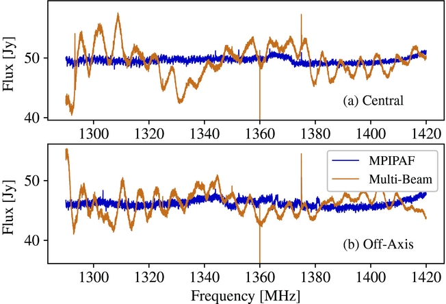
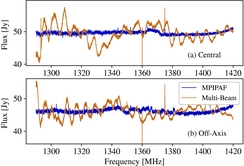
Figure 2. Sample PKS 1934-638 spectra prior to bandpass correction from the MPIPAF (blue) and multibeam (brown) central beam, panel (a), and an off-axis beam, panel (b). The angular offsets of the off-axis beams, MPIPAF beam 1 and multibeam beam 10, are ~0.5° and ~1.5°, respectively. The MPIPAF spectra have been offset by 7 and 27 Jy (the median difference between the MPIPAF and multibeam spectra for the central and off-axis beams, respectively) for ease of comparison with the multibeam spectra.
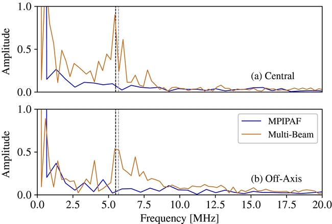
Figure 3. Amplitude of the power in the standing wave spectral feature in the PKS 1934-638 spectra in Figure 2 from Fourier analysis. The amplitude of the standing wave is shown for the MPIPAF (blue) and multibeam (brown) spectra in the central beam, panel (a), and an outer beam, panel (b). The vertical dashed lines indicate 5.5 MHz and 5.7 MHz (black and grey, respectively).
Table 1. MPIPAF and beamformer spectral-line mode specifications for this work.
Table 2. Target fields.
Additionally, we used archival data cubes from the first HIPASS data release (Meyer et al. Reference Meyer2004) and archival Parkes multibeam and ATCA data of the LMC (Staveley-Smith et al. Reference Staveley-Smith, Kim, Calabretta, Haynes and Kesteven2003) for comparison with our HIPASS source and LMC observations, respectively.
We also require optical position and redshift information for potential H i sources to attempt blind H i stacking. We queried the NASA/IPAC Extragalactic Database (NED)Footnote 2 to obtain position and redshift information for optically detected sources within the G23 field, which returned source redshift and positions from the 2DFGRS, GALEXASC, GALEXMSC, and 2MASX surveys.
2.2. Data reduction
We reduced the data using the data reduction and gridding packages livedata and gridzilla Footnote 3 (for a description of livedata and gridzilla, see Barnes et al. Reference Barnes2001). Both livedata and gridzilla are designed for reducing Parkes multibeam data, which are in single dish fits format, sdfits. However, the raw MPIPAF data files are in hdf5 format, so we first converted the hdf5 files to sdfits format using the python package fits2hdf (Price, Barsdell, & Greenhill Reference Price, Barsdell and Greenhill2015). We also separated each of the 16 MPIPAF beams in the raw hdf5 data files into separate sdfits files, as livedata can only conveniently handle up to 13 beams simultaneously (the number of beams in the Parkes multibeam receiver), and reduced each beam separately.
We performed bandpass correction on both the LMC and G23 field data with livedata. Prior to performing bandpass correction, we used PKS 1934-638 to calibrate the flux density scale of the data. We smoothed both data sets using Hanning smoothing and performed bandpass calibration using a second-order robust polynomial and the extended and compact calibration methods for the LMC and G23 data, respectively.
After correcting the bandpass, we gridded the reduced data using gridzilla. We gridded the data using a weighted median, smoothed the data using a Gaussian kernel with full width half maximum (FWHM) of 6 arcmin and a cutoff radius of 13 arcmin and combined the two polarisations. Our final data cubes have a pixel scale of 4 arcmin by 4 arcmin and a spectral resolution of 18.5 kHz.
The Galactic Centre and targeted HIPASS source on-off observations were not reduced using livedata. We reduced these on–off data separately using the on-source and off-source pointings,
 $$\begin{equation}
\begin{array}{l}\displaystyle S_{\nu }=\left(\frac{P_{\mathrm{on},\nu }}{P_{\mathrm{off},\nu }}-1\right)T_{\mathrm{sys}}(\nu ), \end{array}
\end{equation}$$
$$\begin{equation}
\begin{array}{l}\displaystyle S_{\nu }=\left(\frac{P_{\mathrm{on},\nu }}{P_{\mathrm{off},\nu }}-1\right)T_{\mathrm{sys}}(\nu ), \end{array}
\end{equation}$$
where T sys(ν) is the system temperature determined from observing the calibrator PKS 1934-638 prior to observing the science target, P on,ν is the on-source pointing, and P off,ν is the off-source pointing. We accounted for the frequency dependence of T sys.
The one exception to this is the Circinus galaxy, which did not have a calibrator observation prior to or after the science observation on August 5. For Circinus, we used a PKS 1934-638 observation from August 8 as the nearest calibrator observation. However, we believe that the calibration is reliable as only the central beam (beam 8) was used for this observation which was fairly stable over the August and September observations (see Section 3.2 and Figure 5).
We then used gridzilla to grid the reduced Galactic Centre observation similarly to the LMC and G23 field data. However, we gridded each beam separately, using gridzilla’s weighted median statistic, WGTMED, for RFI suppression and used a top-hat smoothing kernel with a FWHM and cutoff radius of 12 and 6 arcmin, respectively. We did not use gridzilla for the targeted HIPASS sources as they lie in RFI-free regions of the spectrum and simply combined the two polarisations from each beam with a python script.
3 RESULTS
3.1. Standing waves
Standing waves are introduced as a result of broadband signals entering the telescope along multiple paths and creating an interference pattern. The principal (on-source) standing wave at Parkes is created by radiation reflecting from the feed towards the apex of the telescope. The frequency interval of this standing wave is c/2F, where F is the focal length (Parkes F/D = 0.41), and corresponds to 5.6 MHz at Parkes. Reflections off other parts of the dish and feed support legs result in standing waves at other frequencies. Standing waves from off-source interference can be even more complex. As with other baseline artefacts, the effect of standing waves can be mitigated by careful calibration. However, this becomes more difficult if the phase or amplitude of the wave shifts over time (Briggs et al. Reference Briggs, Sorar, Kraan-Korteweg and van Driel1997). Both Delhaize et al. (Reference Delhaize, Meyer, Staveley-Smith and Boyle2013) and Kleiner et al. (Reference Kleiner, Pimbblet, Heath Jones, Koribalski and Serra2016) noted the presence of standing waves in Parkes multibeam data and further corrected by fitting and subtracting high-order polynomials from their spectra. Standing waves can even be problematic for radio interferometers (Popping & Braun Reference Popping and Braun2008).
These results can be understood by noting that the amplitude, a, of the standing wave relative to the power in the direct signal, A, is a/A = 2γ, where γ is the voltage ratio of the delayed and undelayed signals. So, a scattered power of only 0.01% will give rise to a standing wave amplitude ratio of 2% for the multibeam, and a scattered power of only 0.0001% will result in an amplitude ratio of 0.2% for the MPIPAF. The large apparent difference in the reflection coefficient of the two receivers (~100) is partly a result of the increased efficiency of the MPIPAF. The higher efficiency of the MPIPAF leaves less energy available for multipath reflections from the feed, but this can explain at most a 1.4 times reduction in reflected power compared to the multibeam, as suggested from a comparison of the measured multibeam (Staveley-Smith et al. Reference Staveley-Smith1996) and MPIPAF (Chippendale et al. Reference Chippendale, Beresford, Deng, Leach, Reynolds, Kramer and Tzioumis2016) feed efficiencies of 50–64% and 64–75%.
However, this cannot be the only factor. We must also consider that the MPIPAF fully samples the focal plane, such that neighbouring beams, which are separated by 15 arcmin on the sky, also have the same high efficiency. On the other hand, the multibeam feed array undersamples the aperture plane, and neighbouring beams are separated by 28 arcmin, or ~2 beamwidths (Staveley-Smith et al. Reference Staveley-Smith1996). Therefore, the efficiency of this receiver for hypothetical beams separated by 15 arcmin is effectively zero – i.e. most incident radiation is reflected. The low MPIPAF standing wave amplitude must therefore be a result of the low amounts of power reflected from the focal area around a given beam, and not just the power reflected from the beam itself. A more accurate analysis of the excellent standing wave performance of the MPIPAF relative to the traditional multibeam array requires a full electromagnetic simulation and diffraction analysis, and is outside the scope of this paper.
Modulation of the primary beam pattern by standing waves on interferometers is a related problem (Popping & Braun Reference Popping and Braun2008). Using APERTIF on the Westerbork Synthesis Radio Telescope, Oosterloo, Verheijen, & van Cappellen (Reference Oosterloo, Verheijen and van Cappellen2010) have shown that this can also been suppressed using PAFs. Aside from the lower standing wave, additional suppression can be obtained by utilising the frequency flexibility inherent in beamforming. For the MPIPAF, the beamformer weights can be adjusted in 1-MHz sub-bands. As the primary reflection standing wave period of 5.6 MHz is well sampled by the 1-MHz resolution of the beamformer and the 90-mm spatial sampling period of the MPIPAF chequerboard at the focal plane (spacing between PAF element feeds) it may be possible to suppress the standing wave even further via more advanced beamforming techniques in the future.
3.2. System temperature
We determined the system temperature, T sys using the calibrator observation of PKS 1934-638 directly preceding the target observations. Chippendale et al. (Reference Chippendale, Beresford, Deng, Leach, Reynolds, Kramer and Tzioumis2016) determined T sys/η for the MPIPAF to be in the range 45–60 K and to be relatively stable between the two measured polarisations from observations with the dish pointing near zenith. In the three months of observing (August–October), however, we find T sys/η to be significantly higher (increasing with decreasing frequency) and less stable, ranging from ~70–140 K (mostly between ~70–110 K), with significant variation between the two polarisations and the observation dates and beams (see Figures 4 and 5). We also note that adjacent beams are separated by 0.25°, or ~1 beamwidth, so there is some overlap. We measure a mean correlation in the spectral noise between adjacent beams, in the same linear polarisation, of ~10%. As expected, this is slightly less than the level of correlation of 13–20% previously measured for adjacent ASKAP BETA beams, which are separated by 0.78°, or ~0.7 beamwidths (Serra et al. Reference Serra2015).
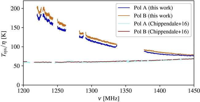
Figure 4. Comparison of polarisation A and B T sys/η variation with frequency for the central beam (beam 8) from October 4 observations with the test values upon installation on Parkes (Chippendale et al. Reference Chippendale, Beresford, Deng, Leach, Reynolds, Kramer and Tzioumis2016). The higher values measured by us at low frequencies are a result of the beamformer delay slips noted in the main text.
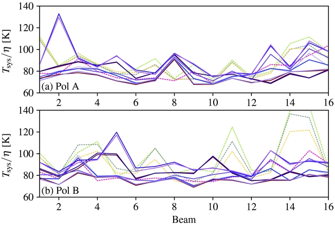
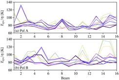
Figure 5. Polarisation A and B T sys/η average values over the frequency range ν = 1400–1420 MHz in each of the 16 beams over observations from August, September, and October (panels (a) and (b), respectively). August and September are dashed lines and October are solid lines.
Some variation in T sys/η is to be expected as new beam weights were not made for each spectral line observation and the state of the hardware was not carefully controlled between observations. The probable cause of the T sys/η variation are delay slips (mostly single-sample) between different ports of the MPIPAF digitiser when the digital receiver is power cycled (Bannister & Hotan Reference Bannister and Hotan2015). In a production system, such as ASKAP or Bonn, this can be calibrated using an on-dish noise source.
The central beam (beam 8) appears to be one of the most stable beams, remaining roughly constant during the August and September observations and at a different value for the October observations (dashed and solid lines Figure 5, respectively). The T sys values for polarisation A were slightly more constant than those for polarisation B. If a PAF is permanently installed on the Parkes telescope, the T sys/η noise can be lowered below the Chippendale et al. (Reference Chippendale, Beresford, Deng, Leach, Reynolds, Kramer and Tzioumis2016) values by cooling the receiver systems. Simulations suggest that a next-generation ‘rocket’ design can achieve T sys/η = 20–25 K (Dunning et al. Reference Dunning, Bowen, Hayman, Kanapathippillai, Kanoniuk, Shaw and Severs2016), which is a 40 K improvement on the MPIPAF and a 15–20 K improvement on the Parkes multibeam receiver.
3.3. Radio frequency interference
There is significant RFI present in the observations, as the Parkes telescope is located in New South Wales and suffers interference from radio, television, mobile phones, as well as satellites. In the frequency range of our observations, the main contributors are the navigational satellite signals (e.g., GPS) at ν < 1290 MHz (see Figure 6). This is in contrast to the excellent RFI situation at the Murchison Radio-astronomy Observatory (MRO) where, with the exception of satellite RFI and tropospheric ducting events (Indermuehle et al. Reference Indermuehle, Harvey-Smith, Wilson and Chow2016), low-frequency observations are largely free of terrestrial contamination.
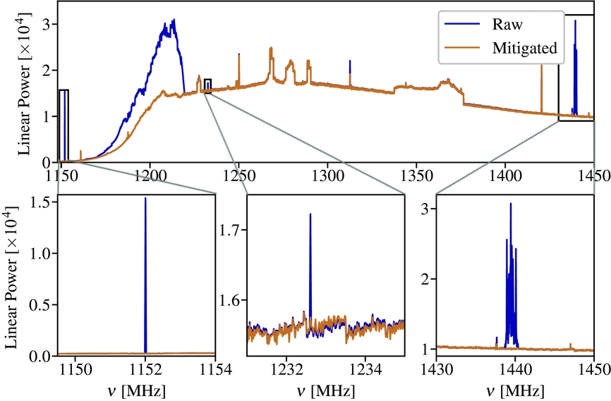
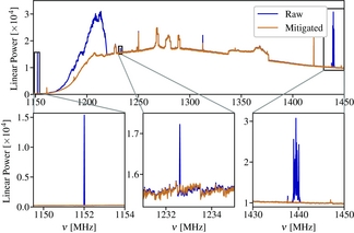
Figure 6. The power spectrum (in arbitrary units) for a sample observation before (blue) and after (brown) applying a realtime projection algorithm for RFI mitigation. Substantial reduction in RFI levels is achieved for the strong RFI signals near 1 150, 1 210, 1 230, 1 310 and 1 440 MHz. We show zoomed-in spectral regions near 1 150, 1 230 and 1 440 MHz in the lower panels. The 1 152 MHz signal is suspected internal RFI and has also been noted in ASKAP spectra. The mitigated signal from 1 159–1219.5 MHz is most likely satellite RFI. The 1232.6 MHz signal is an aliased fundamental of the coarse filter bank readout clock, also noted by Chippendale & Hellbourg (Reference Chippendale and Hellbourg2017). Based on the ACMA Register of Radiocommunications Licenses, the signal at 1439.5 MHz is a telecommunications signal.
Since PAFs can fully sample the focal plane and have flexible beamforming capability, they are perfect for the application of advanced RFI mitigation and suppression techniques (see Fridman & Baan Reference Fridman and Baan2001, for an overview). Indeed, the ASKAP Boolardy Engineering Test Array (BETA) was used to test one of these RFI mitigation methodologies, a spatial filtering technique based on projecting out the interferer signature (Hellbourg et al. Reference Hellbourg, Weber, Capdessus and Boonstra2012). This test demonstrated the effectiveness of the projection algorithm in suppressing RFI contamination in ASKAP PAF data (Hellbourg, Bannister, & Hotarn Reference Hellbourg, Bannister and HotarP2016). This success encouraged us to attempt a similar technique for the MPIPAF data taken at the Parkes site. Full mitigation typically requires much higher temporal and spectral resolution than we have in the MPIPAF data (~ microseconds and ~ kHz vs. 4.5 seconds and 18.5 kHz, respectively). However, we were able to demonstrate again the power of the projection method in some of our observations. (Figure 6 shows spectra taken before (brown) and after (blue) applying RFI mitigation. See Chippendale & Hellbourg Reference Chippendale and Hellbourg2017, for further details)
For most of our observations, RFI contamination was removed from the spectra using more conventional threshold flagging techniques, by excluding individual spectral channels with flux density, S νobs > 5σ i , where σ i is the channel RMS noise. We excluded all optical sources with redshifts placing them within the frequency range of GNSS satellites (1240–1252 MHz). We also excluded, by manual inspection, all spectra containing occasional GPS L3 emissions at 1376–1384 MHz. We did not exclude sources falling within the receiver breakthrough at ~1350 MHz as this appeared relatively stable and, unlike other RFI regions had a reasonably low channel RMS (0.06–0.08 Jy, c.f. clean spectral channels RMS ~0.04 Jy).
3.4. The Large Magellanic Cloud
The LMC was observed as a check of the accuracy of the flux density and frequency calibration of the MPIPAF, as well as a basic check of the reduction pipeline. We compare our results with accurate archival observations from Staveley-Smith et al. (Reference Staveley-Smith, Kim, Calabretta, Haynes and Kesteven2003), which used the Parkes multibeam receiver. As the observed LMC emission is over the range ν ~ 1418–1419.5 MHz, the LMC observations are in the RFI free section of the band and we can use all channels containing LMC emission.
We gridded the MPIPAF data without any further calibration or adjustment except to apply a Gaussian smooth of FWHM = 7 arcmin to remove small residual scanning lines which can still be seen faintly in Figure 7 at −68° < δ < −67°. Unlike the previous multibeam observations, no cross-scans were taken to mitigate against such artefacts.
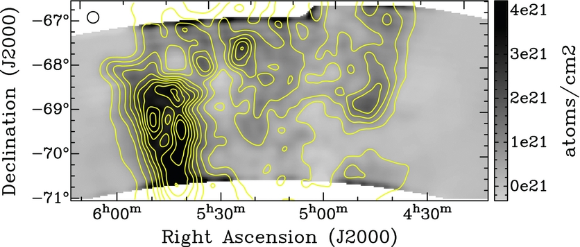
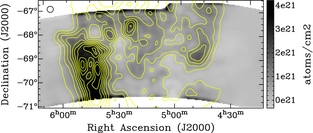
Figure 7. Column density map of the MPIPAF observations of the Large Magellanic Cloud (LMC) overlaid with the yellow contours taken from the archival map from Staveley-Smith et al. (Reference Staveley-Smith, Kim, Calabretta, Haynes and Kesteven2003). The contours are (0.1, 0.2, 0.3, 0.4, 0.5, 0.6, 0.7, 0.8, 0.9) × 5.58 × 1021 atoms/cm−2. The beam size is shown with the black ellipse in the top left corner.
In Figure 7, we compare the MPIPAF column density map with contours from the archival multibeam observations from Staveley-Smith et al. (Reference Staveley-Smith, Kim, Calabretta, Haynes and Kesteven2003). The multibeam contours match well with the MPIPAF image. One thing of note in our map with the MPIPAF data is the edge effects at the top and bottom of the map, which are due to the gridding process under/over-estimating the flux along the edges.
Figure 8 shows a comparison of the brightness temperature values in the individual pixels of the MPIPAF and multibeam image cubes, excluding any boundary regions. There is excellent agreement with the MPIPAF temperature having a small (~1.25 K) zero-point offset. The zero-point offset is mainly due to the in-scan bandpass calibration procedure adopted. This has the effect of removing uniform background emission.
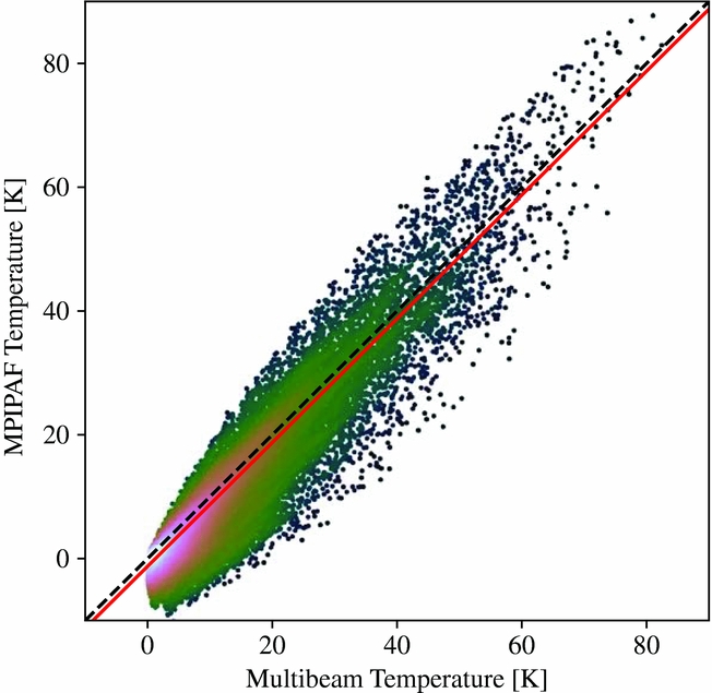
Figure 8. Pixel-by-pixel comparison of temperatures in the MPIPAF and multibeam image cubes. The number of pixels compared is 96,000. The line of best fit is shown in solid red. The shading indicates the data point density, with lighter shading indicating increasing density.
3.5. GAMA G23 field
We extracted the spectrum for each optically identified galaxy listed in NED for the G23 field in the redshift range 0.003 ⩽ z ⩽ 0.23, covering the available bandpass of the MPIPAF band 2. In each channel, we averaged the flux from a 9 pixel box (3 × 3 pixel − 12 × 12 arcmin) centred on the galaxy to ensure we did not lose any flux. We then extracted 600 channels (~11 MHz) around the central redshifted frequency for each galaxy.
3.5.1. H I stacking
We perform H i stacking using the H i mass spectra rather than the originally extracted flux density spectra. We computed the observed-frame H i mass spectrum following Equation 1 from Delhaize et al. (Reference Delhaize, Meyer, Staveley-Smith and Boyle2013),
 $$\begin{equation}
\begin{array}{l}\displaystyle \frac{M_{\mathrm{H{\fontsize{4}{5}\selectfont{{\I}}},\nu _{\mathrm{obs}}}}}{M_{\odot }\,\mathrm{MHz}^{-1}}=4.98\times 10^7\left(\frac{S_{\nu _{\mathrm{obs}}}}{\mathrm{Jy}}\right)\left(\frac{D_L}{\mathrm{Mpc}}\right)^2, \end{array}
\end{equation}$$
$$\begin{equation}
\begin{array}{l}\displaystyle \frac{M_{\mathrm{H{\fontsize{4}{5}\selectfont{{\I}}},\nu _{\mathrm{obs}}}}}{M_{\odot }\,\mathrm{MHz}^{-1}}=4.98\times 10^7\left(\frac{S_{\nu _{\mathrm{obs}}}}{\mathrm{Jy}}\right)\left(\frac{D_L}{\mathrm{Mpc}}\right)^2, \end{array}
\end{equation}$$
where S νobs is the observed-frame flux density and D L is the luminosity distance.
To stack spectra, all spectra must be shifted and aligned at the rest frequency, 1420.406 MHz. We do this by shifting the spectral axis from observed to rest frame [i.e. νrest = νobs(1 + z)] and to conserve total mass,
 $$\begin{equation}
\begin{array}{l}\displaystyle M_{\mathrm{H{\fontsize{4}{5}\selectfont{{\I}}},\nu _{\mathrm{rest}}}}=\frac{M_{\mathrm{H{\fontsize{4}{5}\selectfont{{\I}}}},\nu _{\mathrm{obs}}}}{1+z}. \end{array}
\end{equation}$$
$$\begin{equation}
\begin{array}{l}\displaystyle M_{\mathrm{H{\fontsize{4}{5}\selectfont{{\I}}},\nu _{\mathrm{rest}}}}=\frac{M_{\mathrm{H{\fontsize{4}{5}\selectfont{{\I}}}},\nu _{\mathrm{obs}}}}{1+z}. \end{array}
\end{equation}$$
We compute the stacked H i mass spectrum as done by Delhaize et al. (Reference Delhaize, Meyer, Staveley-Smith and Boyle2013),
 $$\begin{equation}
\begin{array}{l}\displaystyle M_{\mathrm{stacked,{\it i}}}=\frac{\sum _i w_i M_{\mathrm{H{\fontsize{4}{5}\selectfont{{\I}}},\nu _{\mathrm{rest}},{\it i}}}}{\sum _i w_{\it i}}, \end{array}
\end{equation}$$
$$\begin{equation}
\begin{array}{l}\displaystyle M_{\mathrm{stacked,{\it i}}}=\frac{\sum _i w_i M_{\mathrm{H{\fontsize{4}{5}\selectfont{{\I}}},\nu _{\mathrm{rest}},{\it i}}}}{\sum _i w_{\it i}}, \end{array}
\end{equation}$$
where $M_{\mathrm{H{\fontsize{4}{5}\selectfont{{\I}}},\nu _{\mathrm{rest}},i}}$
is an individual galaxy’s H i mass in channel i, M
stacked, i is the final stacked mass in channel i, and w
i
is the weight given by
$M_{\mathrm{H{\fontsize{4}{5}\selectfont{{\I}}},\nu _{\mathrm{rest}},i}}$
is an individual galaxy’s H i mass in channel i, M
stacked, i is the final stacked mass in channel i, and w
i
is the weight given by
 $$\begin{equation}
\begin{array}{l}\displaystyle w_i=\frac{1}{\sigma _i^2 D_L^4}, \end{array}
\end{equation}$$
$$\begin{equation}
\begin{array}{l}\displaystyle w_i=\frac{1}{\sigma _i^2 D_L^4}, \end{array}
\end{equation}$$
where σ i is the RMS noise in channel i, which we calculated using the miriad task imstat. We removed RFI contamination from the extracted spectra as described in Section 3.3 (excluded channels with S νobs > 5σ i and excluded spectra containing GPS satellite RFI at 1376–1384 MHz). We then fit and subtracted a fourth-order polynomial to the stacked spectra to leave a flat baseline in the final spectrum.
We stacked the $M_{\mathrm{H{\fontsize{4}{5}\selectfont{{\I}}}}}$
spectra in redshift bins of 0.05 up to z = 0.20, with the final bin, 0.20 ⩽ z ⩽ 0.23. We determined the RMS noise in the stacked spectra by randomising and reassigning each redshift to a different pair of coordinates from the input NED catalogue, ensuring that no redshift was assigned to its original coordinates. We then extracted and stacked these mock spectra identically to the galaxy spectra. The stacked mock spectra should not result in a positive detection, as our mock spectra are not centred on galaxies, and should give an approximation of the RMS noise. We performed the randomised stacking 10 times in each redshift bin and inspected each mock stacked spectrum for a possible signal mimicking a detection.
$M_{\mathrm{H{\fontsize{4}{5}\selectfont{{\I}}}}}$
spectra in redshift bins of 0.05 up to z = 0.20, with the final bin, 0.20 ⩽ z ⩽ 0.23. We determined the RMS noise in the stacked spectra by randomising and reassigning each redshift to a different pair of coordinates from the input NED catalogue, ensuring that no redshift was assigned to its original coordinates. We then extracted and stacked these mock spectra identically to the galaxy spectra. The stacked mock spectra should not result in a positive detection, as our mock spectra are not centred on galaxies, and should give an approximation of the RMS noise. We performed the randomised stacking 10 times in each redshift bin and inspected each mock stacked spectrum for a possible signal mimicking a detection.
There was no detection in the 0.00 ⩽ z ⩽ 0.05 bin after excluding two direct detections at z = 0.0043 and z = 0.0055 (see Section 3.6.2). Due to the increasing RFI levels at z > 0.10, there were no direct or indirect H i detections in these redshift bins.
We found a detection for ~1100 stacked galaxies at 0.050 ⩽ z ⩽ 0.075. This signal was not found to be mimicked in the mock spectra from random lines of sight. In Figure 9, we plot the stacked galaxy spectrum (blue) and the random mock spectrum (brown). Both spectra exhibit similar residual baseline curvature.
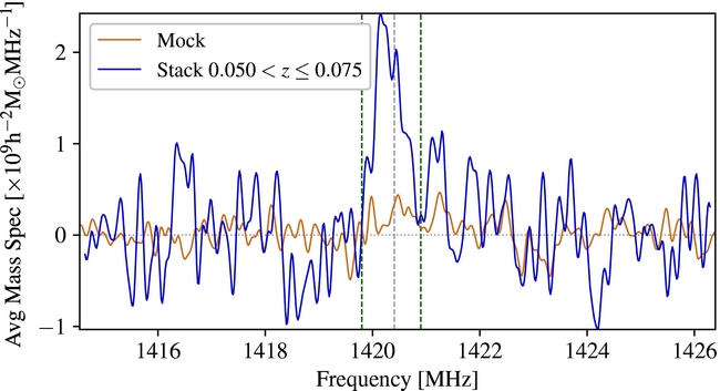
Figure 9. Stacked $M_{\mathrm{H{\fontsize{4}{5}\selectfont{{\I}}}}}$
spectrum (blue) for 1 094 galaxies at 0.05 ⩽ z ⩽ 0.075. The average mock spectrum from randomising the redshifts of the NED catalogue and stacking the spectra (shown in brown). The noise level in the mock spectrum is lower than that of the data as it is the mean of 10 simulations. The dashed green and grey lines indicate the left and right edges of the stacked H i emission determined by visual inspection and the rest frame H i line, respectively.
$M_{\mathrm{H{\fontsize{4}{5}\selectfont{{\I}}}}}$
spectrum (blue) for 1 094 galaxies at 0.05 ⩽ z ⩽ 0.075. The average mock spectrum from randomising the redshifts of the NED catalogue and stacking the spectra (shown in brown). The noise level in the mock spectrum is lower than that of the data as it is the mean of 10 simulations. The dashed green and grey lines indicate the left and right edges of the stacked H i emission determined by visual inspection and the rest frame H i line, respectively.
Our stacked H i detection spans the range from 1419.8–1420.8 MHz (shown in Figure 9 by the dashed green lines), which is significantly narrower than the Delhaize et al. (Reference Delhaize, Meyer, Staveley-Smith and Boyle2013) South Galactic Pole stacked spectra (i.e., ~1 MHz vs. ~3.6 MHz for z = 0.05–0.075 and z = 0.04–0.13, respectively). Our stacked detection is most likely narrower than the results of Delhaize et al. (Reference Delhaize, Meyer, Staveley-Smith and Boyle2013) because of our smaller sample size (i.e., ~1/3 that of the South Galactic Pole region from Delhaize et al. Reference Delhaize, Meyer, Staveley-Smith and Boyle2013) and lower redshift range, hence less confused sources entering our sample.
We integrated over the emission region to calculate the average H i mass of our stacked galaxies using
 $$\begin{equation}
\begin{array}{l}\displaystyle \langle M_{\mathrm{H{\fontsize{4}{5}\selectfont{{\I}}}}}\rangle =\int ^{\nu _2}_{\nu _1} \langle M_{\mathrm{H{\fontsize{4}{5}\selectfont{{\I}}}},\nu }\rangle d\nu , \end{array}
\end{equation}$$
$$\begin{equation}
\begin{array}{l}\displaystyle \langle M_{\mathrm{H{\fontsize{4}{5}\selectfont{{\I}}}}}\rangle =\int ^{\nu _2}_{\nu _1} \langle M_{\mathrm{H{\fontsize{4}{5}\selectfont{{\I}}}},\nu }\rangle d\nu , \end{array}
\end{equation}$$
where ν1 and ν2 are the edges of the emission region. We find an average integrated H i mass of $\langle M_{\mathrm{H{\fontsize{4}{5}\selectfont{{\I}}}}} \rangle = 1.24 \pm 0.18 \times 10^9 h^{-2} M_{\odot }$
. Similar to Delhaize et al. (Reference Delhaize, Meyer, Staveley-Smith and Boyle2013), we computed the error in
$\langle M_{\mathrm{H{\fontsize{4}{5}\selectfont{{\I}}}}} \rangle = 1.24 \pm 0.18 \times 10^9 h^{-2} M_{\odot }$
. Similar to Delhaize et al. (Reference Delhaize, Meyer, Staveley-Smith and Boyle2013), we computed the error in $\langle M_{\mathrm{H{\fontsize{4}{5}\selectfont{{\I}}}}} \rangle$
by integrating the
$\langle M_{\mathrm{H{\fontsize{4}{5}\selectfont{{\I}}}}} \rangle$
by integrating the $\langle M_{\mathrm{H{\fontsize{4}{5}\selectfont{{\I}}}}} \rangle$
random mock stack. We find our
$\langle M_{\mathrm{H{\fontsize{4}{5}\selectfont{{\I}}}}} \rangle$
random mock stack. We find our $\langle M_{\mathrm{H{\fontsize{4}{5}\selectfont{{\I}}}}} \rangle$
value to be lower than the South Galactic Pole value of
$\langle M_{\mathrm{H{\fontsize{4}{5}\selectfont{{\I}}}}} \rangle$
value to be lower than the South Galactic Pole value of $\langle M_{\mathrm{H{\fontsize{4}{5}\selectfont{{\I}}}}} \rangle = 6.93 \pm 0.17 \times 10^9 h^{-2} M_{\odot }$
from Delhaize et al. (Reference Delhaize, Meyer, Staveley-Smith and Boyle2013), indicating we have detected lower mass galaxies.
$\langle M_{\mathrm{H{\fontsize{4}{5}\selectfont{{\I}}}}} \rangle = 6.93 \pm 0.17 \times 10^9 h^{-2} M_{\odot }$
from Delhaize et al. (Reference Delhaize, Meyer, Staveley-Smith and Boyle2013), indicating we have detected lower mass galaxies.
We investigated the noise behaviour of the stacked MPIPAF data by stacking the mock random line of sight flux density spectra, as described previously. We calculated the RMS of a stack of N randomly chosen spectra to determine the noise behaviour with increasing number of stacked spectra. To estimate the noise behaviour, we fix the weighting of each spectra using the mean RMS calculated from 1 000 individual mock spectra (σ = 0.142 Jy) over the frequency range 1321–1352 MHz (corresponding to the redshift range of the stacked H i detection). Figure 10 shows the change in RMS noise in the stacked spectrum with number of spectra included in the stack with the error bars calculated as the 1σ standard deviation of the RMS for 100 random stacks of N spectra. We find the noise decreases as expected for Gaussian noise with a gradient of −0.49 ± 0.01 for the MPIPAF data. This is similar to the noise behaviour for the Parkes multibeam data (gradient ~− 0.5) from Delhaize et al. (Reference Delhaize, Meyer, Staveley-Smith and Boyle2013).
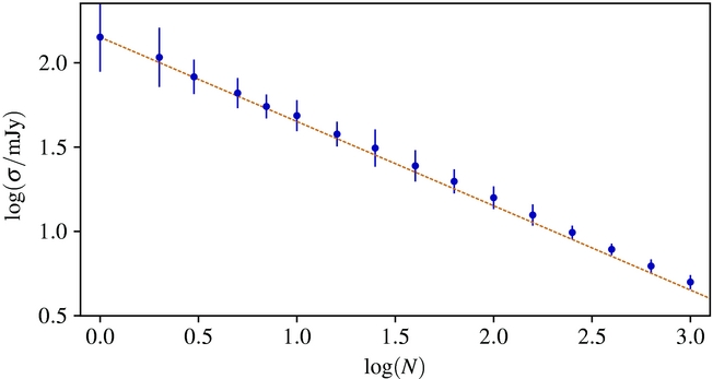
Figure 10. The RMS noise in the stacked flux density signal vs. the number of stacked spectra. The error bars denote 1σ errors on the RMS. The dashed line shows the expected trend, assuming Gaussian noise, in decrease in noise with number of spectra with a gradient of −0.5.
3.6. Comparison with HIPASS detections
We present results of targeted observations of two HIPASS sources, J1413-65 (Circinus) and J1909-63A (NGC 6744) from August 3 and September 4, respectively, observed with the MPIPAF, in addition to two HIPASS sources we detected in the GAMA G23 field, J2242-30 (NGC 7361) and J2309-30 (ESO 469-G015). We obtain HIPASS spectra from the archival HIPASS data cubes from the first HIPASS data release (Meyer et al. Reference Meyer2004).
3.6.1. Targeted HIPASS observations
The Circinus galaxy was only observed with the central MPIPAF beam providing a single spectrum. We therefore compare the MPIPAF observation with the pencil beam spectrum along the same line of sight through the galaxy from the archival HIPASS data cube, as this galaxy is resolved and not contained within a single beam. The MPIPAF and HIPASS spectra agree well in shape and flux density with the only difference in that we detect some additional flux on the high frequency end of the spectrum ( $\nu \rlap{>}{\lower1.0ex\hbox{$\sim $}}1418.5$
MHz, top panel of Figure 11). This is most likely due to a slight position offset between the nearest HIPASS data cube pixel to the MPIPAF spectrum position (HIPASS pixel position: α, δ = 213.41°, − 65.35°, MPIPAF line of sight position: α, δ = 213.36°, − 65.31°).
$\nu \rlap{>}{\lower1.0ex\hbox{$\sim $}}1418.5$
MHz, top panel of Figure 11). This is most likely due to a slight position offset between the nearest HIPASS data cube pixel to the MPIPAF spectrum position (HIPASS pixel position: α, δ = 213.41°, − 65.35°, MPIPAF line of sight position: α, δ = 213.36°, − 65.31°).
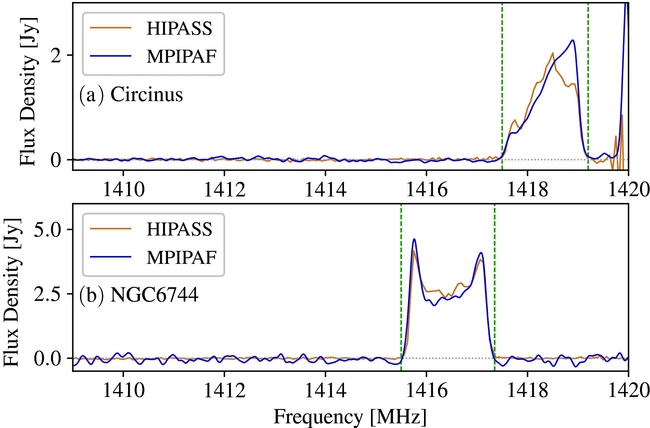
Figure 11. Targeted HIPASS galaxy line of sight spectra of Circinus and NGC 6744, panels (a) and (b), respectively. The Circinus spectrum is from a single line of sight, while the NGC 6744 spectrum is the integrated line of sight spectrum from the 16 MPIPAF beams. The MPIPAF and HIPASS spectra are shown in blue and brown, respectively. The dashed green lines indicate the edges of the galaxy emission determine by visual inspection.
Although the NGC 6744 observation utilized all 16 MPIPAF beams, not all 16 beams lie upon the galaxy. NGC 6744 has an angular radial size in H i of ~15 arcmin (~30 arcmin in diameter, Ryder, Walsh, & Malin Reference Ryder, Walsh and Malin1999), while 13 of the MPIPAF beams have angular separations >30 arcmin from the centre of NGC 6744. We integrated the flux from the three beams with angular separations <24 arcmin. We also calculated the total integrated flux density from the archival HIPASS cube within a 13 × 13 pixel box centred on NGC 6744 (maximum angular separation 24 arcmin, matching the separation of the MPIPAF beams). The spectral shape and flux density of the integrated MPIPAF spectrum agrees with the HIPASS spectrum (lower panel of Figure 11).
3.6.2. G23 H I detections
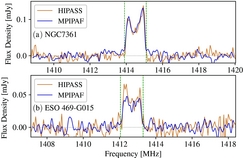
We have two direct H i detections of HIPASS detected galaxies, NGC 7361 and ESO 469-G015, at z = 0.0043 and z = 0.0055 (Figure 12 panels (a) and (b), respectively). We found these direct detections through visual inspection of the H i spectra extracted from the G23 field based on optical identifications from NED. Unlike the targeted HIPASS galaxy observations, we can compare the total integrated flux for these two galaxies as they are completed covered by the drift scan. We compare our MPIPAF spectra with the HIPASS spectra integrated over the same area from the archival data cubes (20 × 20 arcmin) for these two galaxies in Figure 12 (blue and brown lines, respectively). The integrated MPIPAF spectrum of NGC 7361 shows very good agreement with the HIPASS data both in spectral shape and flux density. While the integrated MPIPAF spectrum of ESO 469-G015 has a similar spectral shape, it has a slightly lower flux density. Nevertheless, both spectra agree within the combined uncertainties (Table 3).
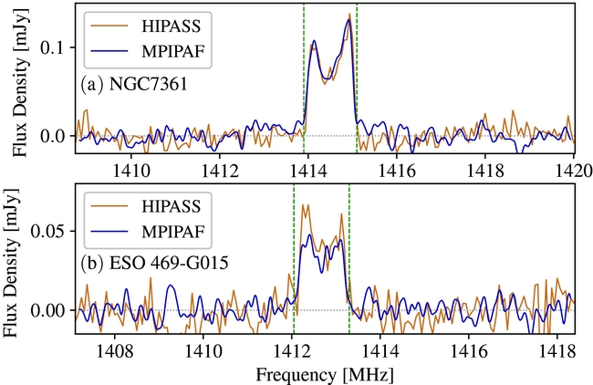
Figure 12. Direct H i detection of HIPASS galaxies NGC 7361 and ESO 469-G015 at z = 0.0043 and z = 0.0055, panels (a) and (b), respectively. The MPIPAF and HIPASS integrated spectra are shown in blue and brown, respectively. The dashed green lines indicate the edges of the galaxy emission determine by visual inspection.
Table 3. Integrated fluxes for MPIPAF and HIPASS galaxy spectra shown in Figure 12.
3.7. Galactic centre hydrogen and positronium recombination lines
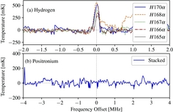
We inspected the Galactic Centre spectra from each beam at the 14 Hydrogen and 11 positronium RRL frequencies predicted from the Rydberg equation within the band (Table 4). We were unable to use large sections of the spectra due to RFI contamination. Also present in the spectra are 1-MHz beamformer ‘jumps’, some of which were not removed during bandpass calibration. These 1-MHz ‘jumps’ have also been seen in early ASKAP data and are not caused by RFI or the Parkes dish, but are due to the discretization of the beamformer weights. We were able to model and remove the spectral shape of the ‘jumps’ with a first-order polynomial fit to each 1-MHz spectral interval as the ‘jumps’ occur at exactly 1-MHz intervals (e.g., 1380.5 MHz, 1381.5 MHz, 1382.5 MHz, etc.). We find detections for the H165α, H166α, H167α, H168α, and H170α hydrogen recombination lines in individual MPIPAF beams (Figure 13(a) shows the stacked signal for these five lines in all 16 MPIPAF beams). In Table 5, we list calculated line parameters from Gaussian fits to the spectra in Figure 13(a). Our calculated peak intensity line temperatures agree with previous single dish Galactic Centre hydrogen RRL studies (Table 5). All other hydrogen recombination lines lie within regions with high RFI contamination and are undetected.
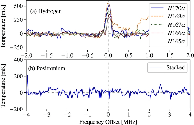
Figure 13. Stacked Galactic Centre hydrogen and positronium spectra, panels (a) and (b), respectively. For hydrogen, we stacked the spectra from all 16 MPIPAF beams, for individual recombination lines and recovered a detection for the 165α, H166α, H167α, H168α, and H170α lines. The positronium spectrum is the combined stack of the Ps131α, Ps132α, Ps133α, and Ps135α lines in all 16 MPIPAF beams and does not show a detection.
Table 4. Rydberg numbers (n) and corresponding hydrogen (H) and positronium (Ps) frequencies.
Table 5. Galactic Centre FWHM line widths and line temperatures (T L) for hydrogen radio recombination line (RRL) detections from (a) this work and T L from previous studies, (b) Roberts & Lockman (Reference Roberts and Lockman1970), (c) Riegel & Kilston (Reference Riegel and Kilston1970), (d) Kesteven & Pedlar (Reference Kesteven and Pedlar1977), (e) Hart & Pedlar (Reference Hart and Pedlar1980).
For positronium, however, we did not have any clear direct detections above the noise. In an attempt to improve the signal to noise, we stacked the Galactic Centre spectra from each beam centred on the predicted frequencies of positronium recombination lines to look for a stacked detection. We were unable to stack spectra at all predicted frequencies due to the presence of RFI, as mentioned above. We excluded the RFI contaminated sections of the spectra. This reduced the number of stacked positronium spectra to 64, centred on the predicted Ps131α, Ps132α, Ps133α, and Ps135α lines. For each spectrum, we extracted 450 channels centred on the predicted line frequency and fit a second-order polynomial to remove the baseline from the stacked spectrum. We find no detection in the stacked positronium spectra in either emission or absorption as shown in Figure 13(b) and set a 3σ upper limit on the stacked recombination line signal of <0.09 K. Using this upper limit, we calculate the recombination rate to be <3.0 × 1045 s−1, assuming the positronium line would have a FWHM of 4.2 MHz, as the positronium line width is thermally broadened to 30 times the hydrogen line width at 1 400 MHz. The positronium upper limit improves upon the results of Anantharamaiah et al. (Reference Anantharamaiah, Radhakrishnan, Morris, Vivekanand, Downes and Shukre1989), who placed a 3σ upper limit of <29.3 K (recombination rate <1.1 × 1044 s−1, assuming a line width FWMH of 4.2 MHz) on the detection of the positronium Ps133α line from the Galactic Centre from VLA observations. It should be noted that the recombination rate upper limit from Anantharamaiah et al. (Reference Anantharamaiah, Radhakrishnan, Morris, Vivekanand, Downes and Shukre1989) is lower than our value due to the differing flux limits (<3.4 mJy vs. <84 mJy from the VLA and Parkes, respectively), which is a result of the arcsecond vs. arcminute resolution of the VLA (~12 × 6 arcsec) and Parkes (~15 × 15 arcmin), respectively.
4 CONCLUSIONS
We have presented results of using a modified ASKAP PAF mounted on the Parkes 64-m radio telescope for performing H i mapping and stacking.
-
• The standing wave amplitude, resulting from interference with reflected waves, is substantially reduced in the PAF data compared with conventional receivers. We estimate an amplitude reduction by a factor of ~10 compared with the multibeam receiver. This reduction represents the higher efficiency and full focal-plane sampling of the PAF.
-
• The system temperatures during our observations are higher and less stable than those during initial tests by Chippendale et al. (Reference Chippendale, Beresford, Deng, Leach, Reynolds, Kramer and Tzioumis2016). This is most likely due to delay slips in the digital receiver which were not monitored or corrected for during the observations, but can be corrected using an on-dish noise source to estimate the delays and applying a compensating phase slope to existing beamformer weights.
-
• The lower frequency (ν < 1290 MHz) data contain significant but well-known satellite RFI contamination. We demonstrate that even with the low temporal and spectral resolution of our observations, significant mitigation is possible.
-
• We have compared observations of the LMC with archival Parkes multibeam data, and found excellent agreement.
-
• We have demonstrated that noise continues to decrease with time for long observations with a PAF. In particular, we find a stacked detection of extragalactic H i in the GAMA G23 field in the redshift range 0.05 ⩽ z ⩽ 0.075.
-
• Two direct H i detections in the GAMA G23 field at z = 0.0043 and z = 0.0055 of NGC 7361 and ESO 469-G015 are also noted. Both integrated spectra show good agreement in spectral shape with archival HIPASS data and the measured fluxes agree within the statistical uncertainties.
-
• From targeted observations of HIPASS sources Circinus and NGC 6744, we found reasonable agreement with the archival HIPASS line of sight spectrum of Circinus. Some of the difference may be due to the different (and not optimal) MPIPAF beam shapes. The integrated line of sight spectrum of NGC 6744 agrees well with the integrated HIPASS spectrum.
-
• We find clear direct detections of five hydrogen recombination lines: H165α, H166α, H167α, H168α, and H170α. We do not find a detection of positronium recombination lines in the Galactic Centre observations, but set a 3σ upper limit of <0.09 K, corresponding to a recombination rate of <3.0 × 1045 s−1.
The above demonstration, whilst limited in scope, demonstrates the viability of PAFs on large single dish telescopes. The main areas that need improvement for a permanent installation are the system temperature, which requires cryogenic cooling, and a mechanism for ensuring a stable and reproducible beamforming methodology in the presence of RFI (Chippendale & Hellbourg Reference Chippendale and Hellbourg2017). The flexible beamforming capability of PAFs is nevertheless enormously powerful and can in itself, as already demonstrated, reduce the impact of RFI.
ACKNOWLEDGEMENTS
This research was conducted by the Australian Research Council Centre of Excellence for All-sky Astrophysics (CAASTRO), through project number CE110001020. The Parkes radio telescope is part of the Australia Telescope National Facility, which is funded by the Commonwealth of Australia for operation as a National Facility managed by CSRIO. The MPIPAF is a collaboration between CSIRO Astronomy and Space Science (CASS) and MPIfR of the Max Planck Society. We wish to thank A. Brown for improving the duty cycle of the 18.5 kHz resolution spectrum integrator, M. Marquarding and E. Troup for contributions to software systems development and integration, particularly for observation and telescope control, and Dr. K. Bannister and C. Haskins for support of software implementation of RFI mitigation. This research has made use of the NASA/IPAC NED which is operated by the Jet Propulsion Laboratory, California Institute of Technology, under contract with the National Aeronautics and Space Administration.