


Introduction
Developments in the single-particle reconstruction technique for obtaining three-dimensional (3D) images of viruses and proteins have revolutionized structural biology over the last decade. Protein structures determined by electron microscopy deposited to the protein data bank have risen from less than 1% of yearly deposits in 2009 to over 10% of yearly deposits in 2017 (Westbrook, Reference Westbrook2017). The resolution of reconstructions is now routinely at or below 3 Å and, therefore, can be used to determine atomic structures (Holubcová et al., Reference Holubcová, Blayney, Elder and Schuh2015; Bartesaghi et al., Reference Bartesaghi, Aguerrebere, Falconieri, Banerjee, Earl, Zhu, Grigorieff, Milne, Sapiro, Wu and Subramaniam2018). The technique was given the ultimate recognition of its progress when three pioneers of the field were awarded the Nobel Prize in chemistry in 2017 (Cressey & Callaway, Reference Cressey and Callaway2017).
The 3D visualization of structures at the atomic scale is a vital in physical sciences as it is in biology, for example, to understand the catalytic behavior, or the optical and electronic properties of nanomaterials (Bals et al., Reference Bals, Batenburg, Verbeeck, Sijbers and Van Tendeloo2007; Nicoletti et al., Reference Nicoletti, De La Peña, Leary, Holland, Ducati and Midgley2013; Slater et al., Reference Slater, Macedo, Schroeder, Burke, O'Brien, Camargo and Haigh2014). While the use of single-particle reconstruction in structural biology has become pervasive, there has been very limited use of the technique in the imaging of inorganic nanoparticles (Azubel et al., Reference Azubel, Koivisto, Malola, Bushnell, Hura, Koh, Tsunoyama, Tsukuda, Pettersson, Häkkinen and Kornberg2014). 3D imaging of inorganic nanoparticles has largely been undertaken using electron tomography (Leary & Midgley, Reference Leary, Midgley, Hawkes and Spence2019), in which images of the same nanoparticle or collections of nanoparticles are collected at multiple sample orientations by tilting the sample with respect to the electron beam. Electron tomography has been used to reconstruct nanoparticles at atomic resolution (Miao et al., Reference Miao, Ercius and Billinge2016) and also to reconstruct nanoparticles as they change morphology over time due to heating (Vanrompay et al., Reference Vanrompay, Bladt, Albrecht, Béché, Zakhozheva, Sánchez-Iglesias, Liz-Marzán and Bals2018; Koneti et al., Reference Koneti, Roiban, Dalmas, Langlois, Gay, Cabiac, Grenier, Banjak, Maxim and Epicier2019). However, electron tomography has two major drawbacks that often prevent it from being used to investigate many key nanoparticle systems. Firstly, multiple image acquisitions typically impart a large cumulative electron dose to nanoparticle samples, which can cause changes to their morphology. For example, we have observed morphology changes in the PtNi nanoparticles used in this experiment when acquiring multiple spectroscopic datasets (Wang et al., Reference Wang, Slater, Leteba, Roseman, Race, Young, Kirkland, Lang and Haigh2019). While it is possible to obtain the 3D structure of metal nanoparticles at atomic resolution, advanced reconstruction algorithms are required to process the small number of projections obtainable before nanoparticles change in structure (Yang et al., Reference Yang, Chen, Scott, Ophus, Xu, Pryor, Wu, Sun, Theis, Zhou, Eisenbach, Kent, Sabirianov, Zeng, Ercius and Miao2017). Secondly, the acquisition and reconstruction procedures can require expert input to achieve optimal resolution, as demonstrated in the preceding reference. As has been seen in structural biology, both of these drawbacks can be summarily addressed using single-particle reconstruction (Lyumkis et al., Reference Lyumkis, Moeller, Cheng, Herold, Hou, Irving, Jacovetty, Lau, Mulder, Pulokas, Quispe, Voss, Potter and Carragher2010; Yan et al., Reference Yan, Cardone, Zhang, Zhou and Baker2014; Henderson, Reference Henderson2015), in which identical structures at different orientations can be used instead of the same structure tilted to different orientations.
We recently reported a single-particle reconstruction approach to reveal the elemental distribution within a PtNi nanoparticle in three dimensions at the nanoscale (Wang et al., Reference Wang, Slater, Leteba, Roseman, Race, Young, Kirkland, Lang and Haigh2019). Although a promising catalytic material, this nanoparticle system was also chosen as it had a highly homogeneous population. For the majority of inorganic nanoparticle systems, however, populations are typically heterogeneous in size and shape. The issue of heterogeneity is not limited to inorganic systems. Heterogeneity has been a limiting factor in the single particle analysis of many protein systems, which can take on numerous configurations. Recently, there have been a number of studies which alter the reconstruction approach to take this heterogeneity into account. For example, assuming a continuum of conformational states in a higher-order manifold (Maji et al., Reference Maji, Liao, Dashti, Mashayekhi, Ourmazd and Frank2020; Moscovich et al., Reference Moscovich, Halevi, Andén and Singer2020) or through the discrete classification of different structures in 2D or 3D (Serna, Reference Serna2019). These techniques could similarly be applied to inorganic nanoparticles, although we have chosen to explore 2D classification methods alone in this study.
A key advantage of inorganic nanoparticles, compared to proteins, is that they are typically both significantly more robust to electron beam irradiation and consist of elements of higher atomic number. This allows acquisition of high signal-to-noise ratio images via annular dark-field (ADF) imaging in a scanning transmission electron microscope (STEM). A higher signal-to-noise ratio facilitates a more straightforward classification of the 2D images, enabling the use of automated classification methods that would be difficult to conduct on single particle images of proteins or viruses. This type of automated classification based on particle properties has been demonstrated numerous times, for example, on populations of gold nanoparticles in transmission electron microscope images (Konomi et al., Reference Konomi, Dhavala, Huang, Kundu, Huitink, Liang, Ding and Mallick2013) and calcium phosphate particles in scanning electron microscope images (Odziomek et al., Reference Odziomek, Ushizima, Oberbek, Kurzydłowski, Puzyn and Haranczyk2017). Furthermore, the high signal-to-noise ratio of input images means that relatively few images are required in each class in order to obtain a high fidelity 3D reconstruction.
In this study, we demonstrate that single-particle reconstruction can be applied to heterogeneous inorganic nanoparticle populations with almost all aspects fully automated. Acquisition of high-angle annular dark-field (HAADF)-STEM images of nanoparticles is performed using an automated acquisition script. Particles are then automatically segmented, before using automated image analysis for clustering of nanoparticles based on a number of particle properties. This allows grouping of nanoparticles into clusters to define homogeneous component populations. We explore the use of three clustering algorithms (K-means, DBSCAN, and OPTICS) in order to determine the optimum choice of algorithm and parameters for our methodology. Clusters of particle images are then processed using standard single-particle reconstruction algorithms to obtain an individual 3D reconstruction for each component in the population.
In order to demonstrate the validity of our approach, we applied the technique to a heterogeneous nanoparticle sample produced by combining three different nanostructures. The component populations were approximately spherical Au nanoparticles with diameters of 15–25 nm, cuboidal Pd nanoparticles with diameters close to 10 nm and etched rhombic dodecahedral (which we refer to as star-shaped) PtNi nanoparticles of approximately 15 nm diameter. While the same approach is applicable to particles of continuous heterogeneity, we used component populations of known morphology so that the techniques employed could be most effectively validated.
Materials and Methods
Nanoparticles Synthesis
Gold nanoparticles of nominally 20 nm diameter were purchased from Sigma-Aldrich (product ref. 741965). PtNi nanoparticles were synthesized using a procedure previously published (Wang et al., Reference Wang, Slater, Leteba, Roseman, Race, Young, Kirkland, Lang and Haigh2019), using the OLEA-aged particles from this previous publication. For the synthesis of the Pd nanocubes, 60 mg of ascorbic acid (≥99.0%, Sigma-Aldrich), 105 mg of polyvinylpyrrolidone (PVP, Sigma-Aldrich, M.W. 55,000 g/mol), 5 mg of KBr (VMR chemicals), and 185 mg of KCl (VMR chemicals) were placed in a 20 mL vial and dissolved in 8 mL of deionized water. The resulting solution was heated in air under magnetic stirring at 80 °C. After 10 min, a solution containing 57 mg of Na2PdCl4 in 3 mL of deionized water was quickly added, and the reaction was allowed to proceed at 80 °C for 3 h. The product was collected by centrifugation and washed two times with acetone and ten times with water to remove excess PVP. All nanoparticle solutions were sequentially deposited dropwise onto a single holey carbon covered copper TEM grid (200 mesh) to create a grid containing all three nanoparticles.
Image Acquisition
HAADF imaging was conducted in a JEOL ARM 200 scanning transmission electron microscope (STEM). All images were acquired with a 200 kV accelerating voltage, approximately 13 pA beam current, 23 mrad convergence angle, and 80 mrad ADF detector inner angle.
The autoSTEM DigitalMicrograph script (Slater, Reference Slater2019) was used to automate ADF-STEM image collection. The first step of this script is to define the imaging area by inputting minimum and maximum stage locations. The script moves the stage to the initial location (if not already there) and performs an auto-focusing routine. The auto-focusing involves taking an image at a range of focus conditions (in this case, ten images evenly separated over 200 nm) and then calculating the sharpness of the auto-correlation of each image. The sharpness of the auto-correlation is then fit with a Gaussian to find the optimal value.
Once the focus value is found, a low-magnification image is taken. The script then divides this image into segments depending on the magnification requested for the final images. Each segment is checked for the presence of nanoparticles using a simple thresholding and peak finding. If nanoparticles are present in the image segment, an image is acquired at the requested resolution using a reduced scan area. Once all of the image segments have been interrogated, the stage is moved to the next position (in a serpentine motion from minimum to maximum position). The procedure is looped over again, beginning with the auto-focusing routine. The procedure is summarized in Figure 1.

Fig. 1. Workflow for automated image acquisition and 3D reconstruction.
Image Segmentation
Once acquired, images were segmented using an automated segmentation routine using a Li threshold (Li & Tam, Reference Li and Tam1998), on images that had already employed a rolling ball filter of size 301 pixels and a 1 pixel Gaussian smoothing. A watershed algorithm was used to separate touching particles, using a minimum seed separation of 40 pixels. Before watershed seed generation, a binary erosion of 10 pixels was used on the thresholded image to generate the distance map for seeding.
Particle Clustering and Reconstructions
Clustering of particles was carried out using a selection of algorithms employed from the scikit-learn python package (Pedregosa et al., Reference Pedregosa, Varoquaux, Gramfort, Michel, Thirion, Grisel, Blondel, Prettenhofer, Weiss, Dubourg, Vanderplas, Passos, Cournapeau, Brucher, Perrot and Duchesnay2011). In all cases, clustering was carried out using particle properties that were normalized to have a variance of one. We have employed K-means, DBSCAN, and OPTICS algorithms for clustering.
K-means clustering operates by minimizing
 $$\sum\limits_{\,j = 1}^k {\sum\limits_{i_l\in C_j} {\vert { {i_l-w_j} \vert } } } ^2$$
where Cj is the jth cluster, il is the lth particle property, wj is the jth centroid property, and k is the number of clusters. This is essentially minimizing the squared distance between particles and cluster centroids in the multi-dimensional property space. In practice, the algorithm does this by iterating between calculating centroid locations and assigning each particle to a cluster based on the squared distance from its centroid.
The DBSCAN clustering algorithm is a density-based clustering algorithm that finds clusters of high-density. Particles are connected when they are within a user-defined minimum distance to a user-defined number of other particles. Clusters are formed from all connected particles. Distances are calculated in a multi-dimensional property space in the same manner as the K-means algorithm, although for distances rather than the square of distances.
The OPTICS algorithm is essentially a generalization of the DBSCAN algorithm that allows the distance between points to vary between each cluster. This allows finding of clusters of different densities. The maximum distance between points in each cluster is set by finding a distance in which a plot of distance versus the number of points reaches its steepest point. A graphical demonstration is shown in the documentation of the scikit-learn package.
Segmentation and clustering using ParticleSpy on the data from this paper can be executed using the binder found at https://mybinder.org/v2/gh/tomslater/automated_SPR_inorganic/master.
Reconstructions were performed using the e2initialmodel program of the EMAN2 software package (Tang et al., Reference Tang, Peng, Baldwin, Mann, Jiang, Rees and Ludtke2007). Octahedral symmetry was imposed on the reconstruction and the highest fidelity reconstruction was taken for each cluster.
Results and Discussion
136 HAADF-STEM images were automatically collected over the course of 4 h (an example of which is shown in Fig. 2b) with no need for manual input after starting the script. Each image took approximately 30 s to acquire, with a majority of the time taken up by the automated focusing routine, saving images and translating the stage, rather than image acquisition.

Fig. 2. Automated imaging and segmentation. (a) Schematics of the steps employed in the automated acquisition script. (b) HAADF-STEM image of a heterogeneous nanoparticle mixture acquired using auto-acquisition software. Three distinct component particle morphologies are visible (roughly spherical Au of 20 nm diameter, cuboidal Pd of 10 nm diameter, and star-shaped PtNi of 15 nm diameter), although there are large variations even within each class of particle. (c) Image showing the successful segmentation and labeling of each particle with a different color after automated segmentation. The colors do not correspond to any particle property and are purely to distinguish individual particles. (d) Properties extracted by ParticleSpy for a single particle in image (b). (e) Plots of the properties of all particles extracted from the image series for one, two, and three properties.
Segmentation and subsequent analysis of particle properties were carried out using a newly developed python package, ParticleSpy (Slater, Reference Slater2020). This package is built to allow analysis of particles from Hyperspy (De La Peña et al., Reference De la Peña, Fauske, Burdet, Ostasevicius, Sarahan, Nord, Taillon, Johnstone, MacArthur, Eljarrat, Mazzuco, Caron, Furnival, Walls, Prestat, Donval, Martineau, Zagonel, Jokubauskas, Aarholt, Garmannslund and Iyengar2019) signal objects. Segmentation can be performed automatically [using wrappers for functions in the scikit-image package (Van Der Walt et al., Reference Van Der Walt, Schönberger, Nunez-Iglesias, Boulogne, Warner, Yager, Gouillart and Yu2014)] or manually using a user interface. Here, we employed an automated segmentation using an Li threshold (Li & Tam, Reference Li and Tam1998) (an example segmented image is shown in Fig. 2b). This initial segmentation step picked out 1337 particles, which is over 70% of all particles present in the 136 HAADF-STEM images.
A key capability of the ParticleSpy package is automated analysis of particle properties. The analysis outputs the area, circularity, solidity (the area of a region divided by the area of its convex hull), major and minor axes lengths, eccentricity, maximum intensity, and total intensity of each particle (see Fig. 2d for example properties of a single particle). These properties can be plotted natively as histograms or 2D/3D scatter plots depending on the number of properties selected to plot (examples of which are shown in Fig. 2e).
We initially attempted to cluster particles using a K-means clustering algorithm (Alsabti et al., Reference Alsabti, Ranka and Singh1997; Fig. 3). Clustering was based on all size and shape measures included in ParticleSpy. K-means clustering aims to find a user-defined number of clusters that have a minimum in inertia. The algorithm works by assigning a specified number of cluster centroids, before assigning each point to a cluster by calculating its closest centroid. The procedure iterates between calculating new centroids for each cluster and reassigning points to each cluster based on the new centroids until clusters no longer change. As the full particle population is made up of three sub-populations we used 3 clusters for K-means clustering initially.

Fig. 3. K-means clustering of three particle types based on their properties and 3D reconstruction from resulting clusters. (a) Distribution of clusters of particles plotted as a function of maximum HAADF intensity within the particle and solidity of the particle. Particle clusters were found using K-means clustering, specifying 3 clusters with all size/shape properties. (b) Images of the first five particles in each of the clusters to be used for reconstructing initial 3D models. Clusters can be seen to not represent one sub-population only, with large heterogeneity in size and shape. (c) Isosurface renderings of the 3D reconstructions from the clusters shown in (a). Colors correspond to each cluster shown in (a). The 3D reconstructions are not representative due to the heterogeneity captured in each cluster.
However, K-means with 3 clusters did not provide reconstructions that matched the expected morphologies of nanoparticles in the sample (reconstructions shown in Fig. 3c). Performing cross-correlation between projections of the 3D reconstructions and particle images in the corresponding cluster resulted in average cross-correlation coefficients between 0.74 and 0.83, lower values than achieved in subsequent clustering procedures. We suggest that the large clusters obtained through this algorithm do not contain particles with sufficient homogeneity in size and shape to provide high fidelity reconstructions. Similarly, performing clustering based only on a select group of properties resulted in similar clusters and reconstructions which did not represent sub-populations (see Fig. 4).

Fig. 4. K-means clustering of particles based on their properties and the resulting 3D reconstructions. (a) Distribution of clusters of particles plotted as a function of maximum HAADF intensity within the particle and solidity of the particle. Particle clusters were found using K-means clustering, specifying 3 clusters with the only area, maximum intensity and solidity properties used for clustering. (b) Isosurface renderings of 3D reconstructions from the clusters shown in (a). Colors correspond to each cluster found. The clusters do not represent the distinct populations due to the heterogeneity of particles in each cluster.
In order to reduce particle heterogeneity within each cluster, we performed K-means clustering with 4 clusters specified instead of 3 (see Fig. 5). In this case, clusters were found that qualitatively represent the three populations but the fourth cluster still contained a heterogeneous mixture of multiple populations. The results from K-means clustering with 4 clusters compared to that with 3 clusters indicate that specifying more clusters produces smaller clusters, with each having increased homogeneity. It should therefore be possible to specify a large number of clusters for K-means clustering, each of which will possess a largely homogeneous population. The drawback is that the choice of cluster number is somewhat arbitrary (although could be defined based on a target number of particles in each cluster) and will always include all particles, including outliers that do not fit into any cluster.

Fig. 5. K-means clustering of four particle types based on their properties and 3D reconstruction from resulting clusters. (a) Distribution of clusters of particles plotted as a function of maximum HAADF intensity within the particle and solidity of the particle. Particle clusters were found using K-means clustering, specifying 4 clusters with all size/shape properties. (b) Isosurface renderings of the 3D reconstructions from the clusters shown in (a). Colors correspond to each cluster shown in (a). The blue, orange, and red clusters are representative of sub-populations but the green cluster encompasses multiple sub-populations.
An alternative approach to clustering is the DBSCAN algorithm and the related OPTICS algorithm, as documented in the scikit-learn python package (Pedregosa et al., Reference Pedregosa, Varoquaux, Gramfort, Michel, Thirion, Grisel, Blondel, Prettenhofer, Weiss, Dubourg, Vanderplas, Passos, Cournapeau, Brucher, Perrot and Duchesnay2011). These algorithms aim to find high-density clusters, ignoring outliers. The DBSCAN algorithm begins by finding high-density cores from which to propagate. The user specifies a minimum number of points which a point must be close to, and the maximum distance by which the point can be from these points (termed epsilon). The algorithm then works outwards from the high-density cores, adding all points that are within epsilon distance of at least the minimum number of other points within that cluster.
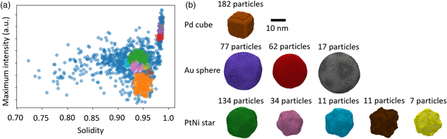
DBSCAN clustering was employed to find homogeneous clusters of nanoparticles based on select properties, namely solidity, maximum intensity, and area (Fig. 6a). The number of minimum connected points and the epsilon value were optimized to provide clusters with a maximum size of 200 particles. Reconstructions from clusters found using this method provided qualitatively closer matches to the morphologies expected (Fig. 6b). A single cluster was found representing Pd cubes, 5 clusters were found representing the PtNi star-shaped particles, and 3 clusters were found representing the Au spheres. In total, 547 of the 1337 particles were included in the found clusters (41% of segmented particles). The cross-correlation coefficients between model projections and particle images were in the range 0.90–0.98, indicating a better match than the K-means clustering algorithm provided.

Fig. 6. DBSCAN clustering of particles based on their properties and resulting 3D reconstructions. (a) Distribution of clusters of particles plotted as a function of maximum HAADF intensity within the particle and solidity of the particle. Particle clusters were found using DBSCAN clustering using only area, maximum intensity, and solidity as properties. (b) Isosurface renderings of the 3D reconstructions from the clusters shown in (a). Colors correspond to each cluster shown in (a). Differences in size within the input nanoparticle sub-populations have been clearly differentiated.
Two of the clusters representing the star-shaped particles (brown and yellow in Fig. 6) can be seen to possess higher levels of noise and match the known morphology of any of the three particle populations. These clusters contain the smallest numbers of particles and, therefore, we suggest that the reconstructions are under-determined. Examination of the clusters suggests that for these reconstructions, which are 166 voxels in all dimensions, approximately 20 particles are required for a high fidelity reconstruction. A robust methodology moving forward would therefore be to remove all clusters that contain fewer than this determined threshold number of particles.
The reconstructions obtained using DBSCAN clustering suggest that not only can the three known sub-populations be found within the data, but these sub-populations can be further divided based on their inherent variability. For example, reconstructions of the three clusters representing the Au spheres show a clear distinction in their size, which represents the variability observed in the particles within the sample population. Similarly, the PtNi clusters show not only a variation in size but also a variation in the solidity of the particles, which would suggest changes in the extent of etching of each particle in their preparation.
Further examples of clustering of particles using DBSCAN and OPTICS algorithms can be found in Figures 7 and 8. In all cases, clusters produce qualitatively higher fidelity reconstructions when the number of particles within them are small enough to give sufficient homogeneity but large enough to provide sufficient sampling of orientations.

Fig. 7. DBSCAN clustering of particles based on their properties and the resulting 3D reconstructions. (a) Distribution of clusters of particles plotted as a function of maximum HAADF intensity within the particle and solidity of the particle. Particle clusters were found using DBSCAN clustering. All properties were used for clustering. (b) Isosurface renderings of 3D reconstructions from the clusters shown in (a). Colors correspond to each cluster found. Representative reconstructions were obtained for all but the orange cluster, which still contains too much heterogeneity to reproduce the known morphology of the star-shaped particles.

Fig. 8. OPTICS clustering of particles based on their properties and the resulting 3D reconstructions. (a) Distribution of clusters of particles plotted as a function of maximum HAADF intensity within the particle and solidity of the particle. Particle clusters were found using OPTICS clustering. All properties were used for clustering. (b) Isosurface renderings of 3D reconstructions from the clusters shown in (a). Colors correspond to each cluster found. The orange and green reconstructions appear to have accurately reconstructed the Au spheres, but all other reconstructions are low-fidelity. All clusters contain relatively few particles and, therefore, provide under-determined reconstructions.
Conclusions
We have demonstrated that single-particle reconstruction can be used to provide 3D reconstructions of heterogeneous inorganic nanoparticle populations. In this particular case, three inorganic nanoparticle systems were combined to create a sample containing three component classes. Clustering of particles found not only the component classes but sub-classes of different sizes and morphologies that could be used to provide individual 3D reconstructions.
We expect this methodology could be performed fully automatically and routinely, from data acquisition to final 3D reconstructions, using existing electron microscope instrumentation and analysis software. The only steps that required manual intervention in the present study were choosing the automated segmentation parameters and selection of the clustering parameters. Definition of the segmentation parameters can initially be performed on a single image and segmentation can then proceed automatically upon collection of each subsequent image. In terms of clustering parameters, the minimum sample and epsilon values should be tailored to provide clusters in an optimal size range for the reconstruction, in this case between 20 and 200 particle images per cluster. The minimum value ensures that orientation space is sufficiently sampled and the maximum value limits cluster heterogeneity at a value that prevents over determination of the reconstruction.
The reconstructions presented in this study possess a resolution on the order of one nanometer. This is of the same order as previous reconstructions from a homogeneous PtNi sample, where a resolution of approximately 7 Å was measured (Wang et al., Reference Wang, Slater, Leteba, Roseman, Race, Young, Kirkland, Lang and Haigh2019). Obtaining atomic resolution reconstructions presents a particular challenge when considering heterogeneous populations, as multiple atomically identical particles would need to be found and clustered together. Currently, this is beyond the methodology presented in this paper. However, it could be possible to obtain the crystallographic orientation of particles, whether through electron diffraction or atomic resolution 2D imaging, and therefore determine the crystallographic orientation of the major facets present in the nanoparticles, as we have previously done for the PtNi particles characterized in this paper (Wang et al., Reference Wang, Slater, Leteba, Roseman, Race, Young, Kirkland, Lang and Haigh2019).
This technique can be employed for the characterization of nanoparticles in an automated and reproducible fashion at the end of a synthesis pipeline. The workflow has the potential to proceed without expert intervention and therefore could be run for extended periods with little supervision. We foresee particular use for this methodology in an industrial setting for quality control of nanoparticle synthesis, alongside its use in a research context to understand the properties of large nanoparticle populations.
Acknowledgments
The authors thank Diamond Light Source for access and support in use of the electron Physical Science Imaging Centre (Instrument E01 and proposal number NT26559) that contributed to the results presented here. S.J.H. and Y.W. acknowledge funding from the European Research Council (ERC) under the European Union's Horizon 2020 research and innovation program under grant agreement No. 715502 (EvoluTEM), the Chinese Scholarship Council and the EPSRC (UK) grant number EP/P009050/1. P.H.C.C. thanks the Jane and Aatos Erkko Foundation and the University of Helsinki for initial support.


 Open access