


1. Introduction
Modelling of coherent structures in turbulent jets has been of interest since pioneering works by Mollo-Christensen (Reference Mollo-Christensen1967) and Crow & Champagne (Reference Crow and Champagne1971) demonstrated the presence of such structures in flows that had previously been considered populated by disorganised turbulent eddies. Among the structures currently considered are the upstream-travelling waves, as discussed in Tam & Hu (Reference Tam and Hu1989) and Towne et al. (Reference Towne, Cavalieri, Jordan, Colonius, Schmidt, Jaunet and Brès2017). Of particular interest among them is the upstream-propagating guided-jet mode ( $k_{p}^{-}$) that is characterised as having a phase speed very close to the speed of sound, maintaining a radial structure outside of the jet core (as such not confined within it) and travelling upstream towards the nozzle (Tam & Hu Reference Tam and Hu1989; Towne et al. Reference Towne, Cavalieri, Jordan, Colonius, Schmidt, Jaunet and Brès2017). For a supersonic jet, at any given set of jet operating conditions this mode will be propagative only within a finite band of frequencies – referred to as the existence region of the mode. The lower bound of this frequency band, where the mode moves away from the sonic line describing free-stream sound waves, is referred to as the branch point (cut-on) and the upper bound as the saddle point (cut-off). The saddle point is formed between the $k_{p}^{-}$ mode and a downstream-propagating duct-like mode ( $k^{+}$) (Towne et al. Reference Towne, Cavalieri, Jordan, Colonius, Schmidt, Jaunet and Brès2017). As the flow parameters are varied, the dynamics of the modes studied here changes significantly: in particular its group velocity. A convectively neutrally stable upstream-travelling mode, the $k^{-}_{p}$ mode, is found only within a finite region in frequency, demarcated by the branch and saddle points. For frequencies above the saddle point, the $k_{p}^{-}$ mode becomes evanescent (spatially decaying).
Recent interest in the  $k_{p}^{-}$ mode has been motivated by the study of aeroacoustic resonance. The feedback loop characterising a given form of resonance consists of four components (Edgington-Mitchell Reference Edgington-Mitchell2019), as shown in figure 1. The first is a downstream-propagating disturbance, often taken to be the Kelvin–Helmholtz (KH) mode, that transports energy to some point downstream of the nozzle. The second is an interaction converting some of this energy to an upstream-propagating disturbance, the third component of resonance. This disturbance travels back to the nozzle where, via another interaction, it excites a new downstream-propagating disturbance. The latter is the last component of the cycle, and which closes the resonance loop. The form of the upstream-propagating component was historically considered to be a free-stream acoustic wave (Powell Reference Powell1953), but recent work has shown that it is instead the $k^{-}$ mode that acts as the upstream component to close the resonance loop. A range of cases that have considered the $k_{p}^{-}$ mode to close resonance include an impinging jet (Tam & Ahuja Reference Tam and Ahuja1990), jet-edge interaction (Jordan et al. Reference Jordan, Jaunet, Towne, Cavalieri, Colonius, Schmidt and Agarwal2018), and screech for both single (Shen & Tam Reference Shen and Tam2002; Edgington-Mitchell et al. Reference Edgington-Mitchell, Jaunet, Jordan, Towne, Soria and Honnery2018; Gojon, Bogey & Mihaescu Reference Gojon, Bogey and Mihaescu2018; Mancinelli et al. Reference Mancinelli, Jaunet, Jordan and Towne2021; Nogueira et al. Reference Nogueira, Jordan, Jaunet, Cavalieri, Towne and Edgington-Mitchell2022b) and twin (Nogueira & Edgington-Mitchell Reference Nogueira and Edgington-Mitchell2021; Stavropoulos et al. Reference Stavropoulos, Mancinelli, Jordan, Jaunet, Weightman, Edgington-Mitchell and Nogueira2023) round jets. For the specific case of screech, high-amplitude and discrete-frequency acoustic tones present in non-ideally expanded jets (Raman Reference Raman1999; Edgington-Mitchell Reference Edgington-Mitchell2019), the finite existence region of the $k_{p}^{-}$ mode then also serves to explain the cut-on and cut-off behaviour of the screech tones (Mancinelli et al. Reference Mancinelli, Jaunet, Jordan and Towne2019; Stavropoulos et al. Reference Stavropoulos, Mancinelli, Jordan, Jaunet, Weightman, Edgington-Mitchell and Nogueira2023). This is because by considering the screech cycle to be closed by the $k_{p}^{-}$ mode, the screech tones can then only be found within the band of frequencies comprising the finite existence region. Recent work by Edgington-Mitchell et al. (Reference Edgington-Mitchell, Wang, Nogueira, Schmidt, Jaunet, Duke, Jordan and Towne2021), following the hypothesis put forth by Tam & Tanna (Reference Tam and Tanna1982), has demonstrated how interactions between the KH mode and the shock-cell structure can result in the creation of new waves, including the $k_{p}^{-}$ mode. Later, in Nogueira et al. (Reference Nogueira, Jaunet, Mancinelli, Jordan and Edgington-Mitchell2022a), it was shown that the KH mode interacts with both the primary and sub-optimal shock-cell wavenumbers to give rise to the $k_{p}^{-}$ mode for different screech tones. As the shock-cell structure exhibits variations in the axial direction (Harper-Bourne & Fisher Reference Harper-Bourne and Fisher1974), sub-optimal wavenumbers represent these variations and appear when taking an axial Fourier transform. This was then generalised by Edgington-Mitchell et al. (Reference Edgington-Mitchell, Li, Liu, He, Wong, Mackenzie and Nogueira2022) to explain the observed screech mode staging (Merle Reference Merle1957; Powell, Umeda & Ishii Reference Powell, Umeda and Ishii1992) in a round single jet.

Figure 1. Illustration of the resonant feedback loop.
The introduction of a second jet introduces additional complexities, as indicated through measurements of inter-jet pressure exceeding twice that of the single-jet value at the same jet distance (Seiner, Manning & Ponton Reference Seiner, Manning and Ponton1988), along with the complex, and often intermittent, coupling behaviour observed (Raman, Panickar & Chelliah Reference Raman, Panickar and Chelliah2012; Bell et al. Reference Bell, Cluts, Samimy, Soria and Edgington-Mitchell2021; Wong et al. Reference Wong, Stavropoulos, Beekman, Towne, Nogueira, Weightman and Edgington-Mitchell2023). In twin-jet systems the jet separation is one of the main parameters governing the dynamics, which now have the tendency to lock into different coupling symmetries about each plane. Prior applications of linear stability theory to the round twin-jet system have shown how these parameters affect the growth rate of the KH mode (Morris Reference Morris1990) and the allowable coupling forms (Rodríguez et al. Reference Rodríguez, Stavropoulos, Nogueira, Edgington-Mitchell and Jordan2023). For the  $k_{p}^{-}$ mode (upstream component in resonance), these parameters also play a role as they have been seen to affect its existence region (Du Reference Du1993; Stavropoulos et al. Reference Stavropoulos, Mancinelli, Jordan, Jaunet, Weightman, Edgington-Mitchell and Nogueira2023). However, there is not currently an explanation as to why this behaviour occurs.
In this work linear stability models will be applied to the supersonic twin-jet case, for both planar and round geometries, to examine the behaviour of the  $k_{p}^{-}$ mode as a function of the jet separation and mode symmetry. By considering changes in frequency of the $k_{p}^{-}$ mode branch and saddle points, and thus, the existence region of the mode, along with their radial structure, an explanation for the dependence of these characteristics on jet separation and mode symmetry will be sought. The approach taken in this work to utilise local, rather than global, models allow for the presented results to be obtained at lower computational cost whilst still providing accurate agreement. It has also been shown (Mancinelli et al. Reference Mancinelli, Jaunet, Jordan and Towne2021; Nogueira et al. Reference Nogueira, Jaunet, Mancinelli, Jordan and Edgington-Mitchell2022a) that local analysis captures several elements of the resonance loop, in particular concerning the characteristics of the different waves that underpin it, with the upstream component being the focus of the current paper.
The paper is organised as follows. The formulations for the numerical models, vortex sheet and finite thickness, utilised are outlined in § 2. Results are shown in § 3, with concluding remarks made in § 4.
2. Mathematical models
2.1. Planar twin-jet vortex-sheet model
The planar twin-jet vortex-sheet model considered builds on the planar single-jet model detailed in Martini, Cavalieri & Jordan (Reference Martini, Cavalieri and Jordan2019). The planar jet is formed using two vortex sheets (Lessen, Fox & Zien Reference Lessen, Fox and Zien1965; Michalke Reference Michalke1970; Morris Reference Morris2010). In the vortex-sheet formulation the axial velocity is constant inside the jet region and zero outside. To extend this to a planar twin-jet configuration, the symmetry line previously imposed at  $y = 0$ for the single-jet case is moved to a position of $y = -H$, the midpoint of the twin-jet system, and no assumptions are made about the symmetry of the flow within each individual jet. This resulting configuration is illustrated in figure 2(a). The two jets are separated by a distance $2H$ and the length scale used for non-dimensionalisation is the jet half-width $h$. A normal-mode ansatz is used to describe pressure fluctuations,
 \begin{equation} \tilde{P} = P(\kern0.7pt y){\rm e}^{{\rm i}(kx-\omega t)}, \end{equation}
where  $k$ is the streamwise wavenumber, $\omega$ is the frequency and $P(\kern0.7pt y)$ is referred to as the pressure eigenfunction. Following Martini et al. (Reference Martini, Cavalieri and Jordan2019) the pressure eigenfunction takes the form
 \begin{equation} P(\kern0.7pt y) = C_{a}{\rm e}^{\lambda_{i,o}y} + C_{b}{\rm e}^{-\lambda_{i,o}y}. \end{equation}
The constants  $C_a$ and $C_b$ in (2.2) are referred to as eigenfunction coefficients, and $\lambda _{i,o}$ is
 \begin{equation} \left. \begin{gathered} \lambda_{i} = \sqrt{k^2 -\frac{1}{T}(\omega-Mk)^2},\\ \lambda_{0} = \sqrt{k^2 -\omega^2}, \end{gathered} \right\} \end{equation}
where  $M$ is the acoustic Mach number and $T$ is the temperature ratio between the jet and free stream. Boundary conditions imposed on the twin-jet system are continuity of pressure and displacement across each vortex sheet, boundedness of the solution as $y \rightarrow \infty$ and the symmetry condition at the midpoint between the two jets ( $y = -H$). This symmetry condition is the solution having either zero gradient (symmetric) or is zero-valued (anti-symmetric). This results in the matrix equation
 \begin{equation} \boldsymbol{\mathsf{A}}(k)\boldsymbol{c} = \boldsymbol{0}, \end{equation}
where
 \begin{equation} \boldsymbol{\mathsf{A}} = \begin{bmatrix} {\rm e}^{-\lambda_{o}} \pm {\rm e}^{{-}2H\lambda_0}{\rm e}^{\lambda_{o}} & -{\rm e}^{-\lambda_{i}} & -{\rm e}^{\lambda_i} & 0\\ \dfrac{\lambda_o}{\omega^2}\left({\rm e}^{-\lambda_{o}} \mp {\rm e}^{{-}2H\lambda_0} {\rm e}^{\lambda_{o}}\right) & \dfrac{-\lambda_{i} {\rm e}^{-\lambda_i}}{\dfrac{1}{T}\left(kM-\omega\right)^2} & \dfrac{\lambda_{i} {\rm e}^{\lambda_i}}{\dfrac{1}{T}\left(kM-\omega\right)^2} & 0\\ 0 & -{\rm e}^{\lambda_i} & -{\rm e}^{-\lambda_i} & {\rm e}^{-\lambda_0}\\ 0 & \dfrac{\lambda_{i}{\rm e}^{\lambda_i}}{\dfrac{1}{T}\left(kM-\omega\right)^2} &\dfrac{-\lambda_{i} {\rm e}^{-\lambda_i}}{\dfrac{1}{T}\left(kM-\omega\right)^2} &\dfrac{\lambda_0}{\omega^2} {\rm e}^{-\lambda_0} \end{bmatrix}, \end{equation}
and  $\boldsymbol {c}$ contains the eigenfunction coefficients
 \begin{equation} \boldsymbol{c} = \begin{bmatrix} C_1\\ C_3\\ C_4\\ C_6 \end{bmatrix}. \end{equation}
The eigenfunction coefficients are related to each flow region through
 \begin{equation} \left. \begin{array}{ll@{}} P(\kern0.7pt y) = C_{1}{\rm e}^{\lambda_{o}y} + C_{2}{\rm e}^{-\lambda_{o}y} & -H< y<{-}h, \\ P(\kern0.7pt y) = C_{3}{\rm e}^{\lambda_{i}y} + C_{4}{\rm e}^{-\lambda_{i}y} & -h< y< h,\\ P(\kern0.7pt y) = C_{5}{\rm e}^{\lambda_{o}y} + C_{6}{\rm e}^{-\lambda_{o}y} & y>h, \end{array} \right\} \end{equation}
where  $C_2$ and $C_5$ have been eliminated prior to forming (2.4) by enforcing the symmetry and bounded boundary conditions, respectively. Setting the determinant of $\boldsymbol{\mathsf{A}}$ equal to zero forms the dispersion relation for the planar twin jet that is used to obtain $k$, the system eigenvalue, for a given set of jet parameters. Once $k$ has been found, (2.4) can then be used to obtain the corresponding eigenfunction coefficients $\boldsymbol {c}$.

Figure 2. Set-up of both the planar (a) and round (b) twin-jet geometries.
For the single planar jet, the dispersion relation given in Martini et al. (Reference Martini, Cavalieri and Jordan2019) is used,
 \begin{equation} \tanh(\lambda_i)^{{\pm} 1} + \frac{1}{T}\left(1-\frac{kM}{\omega}\right)^{2} \left(\frac{\lambda_o}{\lambda_i}\right) = 0, \end{equation}
with the pressure eigenfunctions given by
 \begin{equation}
P(\kern0.7pt
y)=\begin{cases} \dfrac{{\rm e}^{\lambda_i}\pm {\rm
e}^{-\lambda_i}}{{\rm e}^{-\lambda_o}}{\rm e}^{-\lambda_o
y}, & y \geq h,\\ {\rm e}^{\lambda_i y} \pm {\rm
e}^{-\lambda_i y}, & -h \leq y \geq h,\\ \dfrac{{\rm
e}^{-\lambda_i}\pm {\rm e}^{\lambda_i}}{e^{-\lambda_o}}{\rm
e}^{\lambda_o y}, & y \leq{-}h, \end{cases}
\end{equation}
\begin{equation}
P(\kern0.7pt
y)=\begin{cases} \dfrac{{\rm e}^{\lambda_i}\pm {\rm
e}^{-\lambda_i}}{{\rm e}^{-\lambda_o}}{\rm e}^{-\lambda_o
y}, & y \geq h,\\ {\rm e}^{\lambda_i y} \pm {\rm
e}^{-\lambda_i y}, & -h \leq y \geq h,\\ \dfrac{{\rm
e}^{-\lambda_i}\pm {\rm e}^{\lambda_i}}{e^{-\lambda_o}}{\rm
e}^{\lambda_o y}, & y \leq{-}h, \end{cases}
\end{equation}
where the  $\pm$ terms in (2.8) and (2.9) indicate symmetric or anti-symmetric solutions, about the jet centre, respectively.
2.2. Finite-thickness model
The finite-thickness model follows the formulation used previously for round twin-jet systems (Nogueira & Edgington-Mitchell Reference Nogueira and Edgington-Mitchell2021; Stavropoulos et al. Reference Stavropoulos, Mancinelli, Jordan, Jaunet, Weightman, Edgington-Mitchell and Nogueira2023). The two jets, each of diameter  $D$, are separated by a centre-to-centre distance $S$ as illustrated in figure 2(b). Solutions for the twin-jet system are denoted as either SS, SA, AS, or AA, where each letter denotes symmetry (S) or anti-symmetry (A) about the $x$–
$x$– $y$ and $x$–
$x$– $z$ planes, respectively (Rodríguez, Jotkar & Gennaro Reference Rodríguez, Jotkar and Gennaro2018). All parameters are non-dimensionalised by $D$, free-stream sound speed and density. The generalised eigenvalue problem can be expressed, here in terms of pressure, in the form
 \begin{equation} \boldsymbol{L}\hat{P} = k\boldsymbol{R}\hat{P}, \end{equation}
with  $\hat {P} = P\textrm {e}^{\textrm {i}\mu \theta }$ and operators $\boldsymbol {L}$ and $\boldsymbol {R}$ functions of the mean flow, its derivatives, and flow variables $\omega$, $M_{j}$, $S$ and the ratio of specific heats $\gamma$. Here, $\mu$ is the Floquet exponent resulting from the Floquet ansatz that is associated with the different symmetries of the flow (Nogueira & Edgington-Mitchell Reference Nogueira and Edgington-Mitchell2021), $\mu = 0$ describes a solution that is symmetric about the $x$–
$x$– $z$ plane and $\mu = 1$ is anti-symmetric about it. Equation (2.10) utilises a Fourier discretisation in azimuth and Chebyshev polynomials in radius (Trefethen Reference Trefethen2000), with boundary conditions imposed following previous works (Nogueira & Edgington-Mitchell Reference Nogueira and Edgington-Mitchell2021), with the full matrix operators detailed in Stavropoulos et al. (Reference Stavropoulos, Mancinelli, Jordan, Jaunet, Weightman, Edgington-Mitchell and Nogueira2023). A numerical mapping (Bayliss & Turkel Reference Bayliss and Turkel1992) is applied to ensure appropriate resolution in the shear layer of the jets. The sparsity of the system is exploited to further reduce computational cost. The mean flow for each jet is modelled as a hyperbolic-tangent velocity profile (Michalke Reference Michalke1971) of the form
 \begin{equation} U(r) = M\left[0.5+0.5\tanh\left(\left(\frac{R_{j}}{r}-\frac{r}{R_{j}}\right)\frac{1}{2\delta}\right)\right], \end{equation}
with  $R_{j}$ the ideally expanded jet radius and $\delta$ used to characterise the shear-layer thickness. In each case, the mean temperature is obtained from (2.11) through the Crocco–Busemann relation. A twin-jet mean flow is constructed through the addition of two single-jet mean flows, following Rodríguez (Reference Rodríguez2021). When considering instead an elliptical geometry, which will be used as a comparison to the merged round twin-jet system in § 3.2, (2.11) is used with $R_j = R_b$, the boundary curve describing the ellipse
 \begin{equation} R_b = \frac{ab}{\sqrt{b^{2}\cos^{2}(\theta)+a^{2}\sin^{2}(\theta)}}. \end{equation}
Here  $b$ is the ellipse semi-minor axis, and $a$ is both the semi-major axis and the length scale used in normalisation for the ellipse. An example of a single elliptical jet mean flow using (2.12) and (2.11) is provided in figure 3, for an ideally expanded jet Mach number ( $M_j$) of 1.16, $\delta = 0.2$ and aspect ratio (AR) of 2.

Figure 3. Sample elliptical jet mean flow,  $U$, used for the finite-thickness model. Computed for $M_j = 1.16$, $\textrm {AR} = 2$ and $\delta = 0.2$.
3. Results
3.1. Planar twin jet
To aid in understanding the behaviour of a round twin-jet system, a planar twin-jet system, as described in § 2.1, is considered first. For two jets being brought together to the point of merging, the simplified geometry of the planar case allows for a more intuitive understanding of the result. As the planar jets merge they are expected to form a single planar jet, whose width is twice that of the individual planar jets. The effect on the structure of the pressure eigenfunction as the two jets merge ( $H \rightarrow 1$) is shown in figure 4 for both the symmetric and anti-symmetric solutions, respectively. In each case the wavenumber of the $k_{p}^{-}$ (0, 2) mode is found through (2.4). Here the classification (0, 2) follows the form $(m,n_r)$, with $m$ the azimuthal mode number and $n_r$ the number of anti-nodes in the pressure eigenfunction, as defined previously for round jets (Tam & Hu Reference Tam and Hu1989). The same classification will be used to refer to the equivalent mode of the planar system. The primary difference observed between the symmetric (figure 4a–d) and anti-symmetric (figure 4e–h) eigenfunctions is the enforced symmetry condition at the midpoint of the system, which is consistent with results seen for a round twin-jet system (Stavropoulos et al. Reference Stavropoulos, Mancinelli, Jordan, Jaunet, Weightman, Edgington-Mitchell and Nogueira2023). It is observed in both cases that as $H$ decreases the eigenfunctions approach a higher-order mode shape, with additional anti-nodes in the pressure eigenfunctions when $H = 1$ (figure 4d,h). This higher-order mode the system reduces to (for $H = 1$) differs depending on whether the symmetric or anti-symmetric solution is considered. In the symmetric case (figure 4a–d) the amplitude at the midpoint between the jets increases with $H$ before forming an anti-node. Conversely, the symmetry condition for the anti-symmetric case forces a node to form at the centre (figure 4e–h). This results in the anti-symmetric case converging to a mode of greater radial order than the symmetric case.

Figure 4. Variation in structure of the symmetric (a–d) and anti-symmetric (e–h) planar twin-jet pressure eigenfunctions of the  $k_{p}^{-}$ (0, 2) as the two jets merge ( $H \rightarrow 1$). Computed for $M_j = 1.16$, $T$ computed through an isentropic relation, and $St = 0.25$ (a–d), 0.27 (e, f) and 0.3 (g,h). Eigenfunctions are normalised by their maximum absolute value. The inter-jet region is shaded in grey. For the case of $H = 1$ (d,h), the single-jet eigenfunction is overlaid. Results are shown for (a) $H = 20$, (b) $H = 5$, (c) $H = 1.5$, (d) $H = 1$, (e) $H = 20$, ( f) $H = 5$, (g) $H = 1.5$, (h) $H = 1$.
A direct comparison between the twin-jet system at  $H = 1$ and double-width jet can be seen in figure 4(d,h) for the symmetric and anti-symmetric eigenfunctions, respectively. The double-width jet is defined as a single planar jet with half-width $2h$, solved for using the dispersion relation for a single planar jet, (2.8), but for a $St$ twice that of the twin-jet case, due to the present formulation normalising by jet half-width that then becomes $2h$. For both the symmetric and anti-symmetric case in figure 4, the twin-jet solution matches exactly with the double-width jet. This indicates that the converged mode for $H = 1$ corresponds to a mode of the double-width jet. That is, the system is seen to reduce to that of a single planar jet with half-width $2h$.
$2h$.
This consideration of the eigenfunction structure of a planar twin-jet system as  $H \rightarrow 1$ identified key behaviours. When the planar twin-jet system merges it becomes equivalent to a single planar jet of twice the width. At the point of merging ( $H = 1$) the pressure eigenfunction converges to a higher-order mode. For the symmetric case, as the two jets merge, a mode that previously had three peaks on each isolated jet forms a mode with five peaks in the merged jet ( $H = 1$). An equivalent mode for the anti-symmetric case forms a mode with six peaks, indicating the formation of a greater radial order mode than the symmetric case.
This convergence to the double-width jet solution of the twin jet as  $H \rightarrow 1$ can also be observed when considering the branch and saddle point frequencies of the $k_{p}^{-}$ $(0,2)$ mode. It has been observed previously that the existence region formed by these bounds is strongly dependent on jet separation for a round twin-jet system (Du Reference Du1993; Stavropoulos et al. Reference Stavropoulos, Mancinelli, Jordan, Jaunet, Weightman, Edgington-Mitchell and Nogueira2023), and this is also seen to be the case for a planar twin-jet system. Figure 5 shows the change in value of the branch and saddle points for both the symmetric and anti-symmetric case. For both symmetries, the branch and saddle point values are seen as being equal to those of the symmetric planar single jet for large values of H. This is not unexpected when considering figure 4, where it can be observed that, for large $H$, the twin-jet eigenfunctions resemble two symmetric planar jets. As $H \rightarrow 1$, figure 5 shows the twin-jet branch and saddle points approach new values. The exception to this being figure 5(a), the symmetric solution saddle point, which remains virtually unchanged for all $H$. The values to which the branch and saddle points converge to are all related to the double-width jet, being exactly half the values of the single-jet branch and saddle points. Recalling that an equivalent double-width jet has a $St$ value twice that of a planar twin-jet mode, then figure 5 is indicating that when the twin-jet system merges ( $H = 1$), the branch and saddle points change to match those of the higher-order mode of the single-jet configuration that the system has converged to. This equivalence in eigenvalues can also be shown to hold when varying jet parameters, or considering other flow structures, as would be expected. The theoretical equivalence between single and twin planar jets as $H \to 1$ is shown in Appendix A.

Figure 5. Branch and saddle points for the symmetric and anti-symmetric planar twin jet as a function of jet spacing  $H$ at $M_j = 1.16$ and $T$ from an isentropic relation. Present also in each figure is the corresponding value of the symmetric single planar jet. Here the $St$ values converged to at $H = 1$ correspond to half those of the double-width jet. Results are shown for the (a) symmetric branch points, (b) symmetric saddle points, (c) anti-symmetric branch points, (d) anti-symmetric saddle points.
The explanation for the  $k_{p}^{-}$ $(0, 2)$ mode branch and saddle point behaviour in a planar twin-jet system now motivates the investigation of the round twin-jet system.
3.2. Round twin jet
For the round twin-jet system, it has been seen previously that the SA symmetry  $k_{p}^{-}$ $(0, 2)$ mode exhibits a strong dependence on jet separation (Stavropoulos et al. Reference Stavropoulos, Mancinelli, Jordan, Jaunet, Weightman, Edgington-Mitchell and Nogueira2023).The behaviour of both the SS and SA symmetry round twin-jet branch points are compared with those of the symmetric and anti-symmetric planar twin-jet system in figure 6. Results for the round twin-jet system are obtained using (2.10) and (2.11) with $\delta = 0.2$. In the SA (figure 6a) and planar anti-symmetric (figure 6b) systems the branch points both exhibit a strong exponential trend as the jets are brought together. This exponential trendline is of the form $ae^{bx}+c$, with the parameter values as described in table 1. A similar agreement in trends can be seen between the SS (figure 6c) and planar symmetric (figure 6d) branch points. Here the branch points exhibit a constant trend with jet separation and only at very low jet separations is there a change (being at lower jet separation than previous considerations of the SS $k_{p}^{-}$ $(0, 2)$ mode Du Reference Du1993; Stavropoulos et al. Reference Stavropoulos, Mancinelli, Jordan, Jaunet, Weightman, Edgington-Mitchell and Nogueira2023). This change is greater for the SS round twin jet than the symmetric planar twin jet. The similarity in trends of figure 6 suggests that the round twin-jet system is also converging to an equivalent geometry, when $S = 1$, and that drives this change in branch point frequency in a manner analogous to that of the planar jet system. The behaviour of the round twin-jet pressure eigenfunctions can then also be considered, as $S \rightarrow 1$. These are presented in figure 7 for both the SS and SA symmetries at $M_j = 1.16$ and $\delta = 0.2$. As the two round jets are brought together, the SA symmetry condition enforced at the system midpoint becomes an additional node as part of a higher-order mode. This is the same behaviour as was observed previously for the anti-symmetric planar twin-jet system (figure 4). The SS symmetry condition enforced at the system midpoint becomes an anti-node and the twin-jet system reduces to a higher-order mode, again in-line with observations of the planar twin jet (figure 5). Comparing the SS and SA eigenfunctions at $S = 1$ (figure 7d,h), the same difference as previously identified for the planar twin-jet system (§ 3.1) is observed, with the SA solution converging to a greater radial order mode than the SS solution. Figure 7 further indicates that the round twin-jet system approaches a yet-unknown equivalent geometry.

Figure 6. Dependence of the  $k_{p}^{-}$ $(0, 2)$ branch point with jet separation for both the SA (a) and SS (c) round twin jet, and the anti-symmetric (b) and symmetric (d) planar twin jet. Computed for $M_j = 1.16$ and $\delta = 0.2$ (round twin jet). Overlaid on (a,b) is an exponential trendline, with a constant trendline on (c,d). Results are shown for the (a) SA round, (b) anti-symmetric planar, (c) SS round, (d) symmetric planar.
Table 1. Value of parameters for the exponential trendline fitted to the branch points in figure 6.


Figure 7. Variation in structure of the SA (a–d) and SS (e–h) round twin-jet pressure eigenfunctions of the  $k_{p}^{-}$ $(0, 2)$ mode as the two jets merge ( $S \rightarrow 1$). Computed for $M_j = 1.16$ and $\delta = 0.2$. Values of $St$ are 0.595 (a), 0.64 (b), 0.665 (c), 0.695 (d), 0.555 (e), 0.565 ( f), 0.57 (g) and 0.58 (h). Eigenfunctions are normalised by their maximum absolute value. The inter-jet region is shaded in grey. Results are shown for (a) SA, $S = 5$; (b) SA, $S = 2$; (c) SA, $S = 1.5$; (d) SA, $S = 1$; (e) SS, $S = 5$; ( f) SS, $S = 2$; (g) SS, $S = 1.5$; (h) SS, $S = 1$.
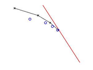
The geometry of a round twin-jet system does not lend itself to an obvious equivalent geometry when the two jets merge, unlike the planar twin-jet system discussed previously (§ 3.1). Instead a comparison will be made with ellipses of differing AR. The two ARs considered are 1.5 and 2, with each shown superimposed over the  $S = 1$ round twin-jet system in figure 8. The AR 1.5 case (figure 8a) provides a match with a large extent of the round twin-jet system, whilst the AR 2 case (figure 8b) is an ellipse of equal area to the twin-jet system. The $S = 1$, SA round twin-jet existence region is compared with ( $k, St$) pairs computed for the elliptical jet, using (2.12) to define the mean flow, in figure 9. Here, the parameters were chosen as $M_j = 1.16$ and $\delta = 0.2$, with $\mu = 0, 1$ for the ellipse and $S = 1$ for the twin jet. In figure 9 both the $St$ and $k$ values for the round twin-jet system are scaled by a factor of $\sqrt {{\textrm {AR}}/{2}}$ (the ratio between the semi-major axis of the ellipse and the diameter of the single jet, used in the twin-jet computations, when considering an equivalent diameter for both the ellipse and merged twin jet) to keep the normalisation consistent between the two cases. It can be seen that of the ARs considered, the merged round twin-jet system more closely resembles the AR $2$ ellipse (figure 9b,d). This is evident from the close agreement observed at the region near the branch point, and the similar behaviour of the twin jet and elliptical jet mode branches. Conversely in the AR 1.5 case (figure 9a,c) the existence regions for the elliptical and round twin jet do not show alignment. Note that this is not implying that a round twin-jet system converges to a perfect ellipse, but that an AR $2$ ellipse could be considered a close approximation to the resultant converged geometry in the context of the existence region. When looking across a larger range in $St$, figure 10 shows that while this agreement is strong at moderate $St$ values, it will begin to lessen as the $St$ value increases. For these lower $St$ values, the associated wavelengths will be larger than the characteristic lengths of the jet. Investigating other geometries at these $St$ values with similar ARs, in particular a rectangular jet geometry, may also lead to similar agreement as observed in figure 9 and could be considered in future studies.

Figure 8. Geometric comparison between the  $S = 1$ round twin-jet system and an elliptical jet of AR 1.5 (a) and 2 (b).

Figure 9. Comparison of the existence regions of the SS and SA,  $S = 1$ round twin-jet $k_{p}^{-}$ (0, 2) mode and the $\mu = 0$, 1 elliptical jet mode branch it lies closest to. Computed for $M_j = 1.16$, $\delta = 0.2$, and $\textrm {AR} = 1.5$ (a,c) and 2 (b,d). Values of $St$ for the twin-jet system are scaled to match the normalisation of the elliptical $St$. Included also is the sonic line representing the free-stream acoustic waves in red. Results are shown for (a) SA, $\mu = 1$, $\textrm {AR} = 1.5$; (b) SA, $\mu = 1$, $\textrm {AR} = 2$; (c) SS, $\mu = 0$, $\textrm {AR} = 1.5$; (d) SS, $\mu = 0$, $AR = 2$.

Figure 10. Comparison of the SA,  $S = 1$ round twin jet and the $\mu = 1$ elliptical jet across a larger $St$ range than considered in figure 9. Computed for $M_j = 1.16$, $\delta = 0.2$ and AR = 2. Values of $St$ for the twin-jet system are scaled to match the normalisation of the elliptical $St$. Included also is the sonic line representing the free-stream acoustic waves in red.
Considering just the AR  $2$ case, comparisons between the mean flows for the ellipse and round twin jet can be made to further compare the similarities. Both mean flows are illustrated in figure 11 for the elliptical (a) and round twin jet (b), respectively. These are computed for $M_j = 1.16$, $\delta = 0.2$, AR = 2 (ellipse) and $S$ = 1 (round twin jet). A qualitative view of figure 11 indicates that the two mean flows are quite different, particularly in their respective behaviour close to the $z$ axis. A more quantitative comparison is made in figure 12 where the velocity profiles are compared along multiple angles, $\theta$, measured from the $y$ axis (see figure 2b). For lower $\theta$ (figure 12a–d), there is strong agreement observed between the two mean flows. It is only at larger $\theta$ (figure 12e, f) that the two mean flows display noticeable difference. As such, this provides a strong justification for considering an AR 2 ellipse as a substitute for the equivalent geometry of a merged round twin-jet system.

Figure 11. Visual comparison of the mean flows for an AR 2 ellipse (a) and  $S=1$ twin jet (b). Computed for $M_j = 1.16$ and $\delta = 0.2$.

Figure 12. Comparison of mean flow axial velocity profiles between the AR 2 ellipse and  $S=1$ twin jet. Computed for $M_j = 1.16$, $\delta = 0.2$ for different $\theta$ all measured from the positive $y$ axis. Results are shown for (a) $\theta = 0$, (b) $\theta = 18$, (c) $\theta = 36$, (d) $\theta = 54$, (e) $\theta = 72$, ( f) $\theta = 90$.
Further comparisons are made by considering the pressure eigenfunctions between the ellipse and round twin jet. These are given in figure 13 at the branch point, for the radial profile along the  $y$ axis (figure 13a,b) and the pressure contours (figure 13b–d). In figure 13(a) the shape of the eigenfunctions agree well between the elliptical and twin-jet solutions. The difference between the $\mu =1$ ellipse and SA round twin jet is in the eigenfunction amplitudes, with the first and third nodes having greater magnitude for the ellipse than the round twin jet. When considering instead the $\mu =0$ ellipse and SS round twin jet (figure 13b), a greater degree of difference is observed between the two eigenfunctions. For $y/D>1$, the elliptical eigenfunction decays at a slower rate than the twin-jet eigenfunction, and at $y/D=0$ there is no match between the two. Comparing the pressure contours for the $\mu =1$ ellipse and SA round twin jet (figure 13c,d) indicates a similar location for the maximum pressure with differences in the contours occurring outside of this region. This is similarly observed when comparing the $\mu =0$ ellipse and SS round twin jet (figure 13e, f). In both cases greater differences between the elliptical and twin-jet contours are seen near to the $z$ axis ( $\theta$ close to ${{\rm \pi} {}}/{2}$ as described by figure 2b). This result is consistent with the previous comparisons of mean flow velocity profiles between the ellipse and $S=1$ round twin jet (figure 12), where it is observed that differences between the velocity profiles occur for values of $\theta$ close to ${{\rm \pi} {}}/{2}$. Trends in the pressure eigenfunction radial profiles, from branch point to saddle point are compared in figure 14. For the SA round twin jet (figure 14a) and $\mu =1$ ellipse (figure 14b), both are seen to display similar behaviour in the pressure eigenfunction as $St$ increases towards the saddle point value. Differences between the two geometries are observed in the pressure eigenfunction amplitudes and the profile at the saddle point. When considering the SS round twin jet (figure 14c) and $\mu =0$ ellipse (figure 14d), similar agreement between the geometries is observed; however, at $y/D=0$ the SS twin jet increases in amplitude as $St$ increases to a larger extent than the $\mu =0$ ellipse does. Combined figures 13 and 14, like figure 9, indicate that an equivalent geometry a round twin-jet system merges to is close in shape to an AR $2$ ellipse.

Figure 13. Pressure eigenfunctions of the  $\mu$ = 0 and 1 ellipses, and the SS and SA, $S = 1$ round twin jet computed at the branch point. Shown for the radial profile (a,b), anti-symmetric contours (c,d) and symmetric contours (e, f). Computed for $M_j = 1.16$ and $\delta = 0.2$. Eigenfunctions are normalised by their maximum absolute value. Results are shown for the (a) anti-symmetric, (b) symmetric, (c) SA twin jet, (d) $\mu = 1$ ellipse, (e) SS twin jet, ( f) $\mu = 0$ ellipse.

Figure 14. Comparison of the pressure eigenfunction behaviour between the  $S = 1$ round twin jet (a,c) and the AR 2 ellipse (b,d), when moving from the branch to saddle point. Computed for $M_j$ = 1.16, $\delta = 0.2$ and AR = 2. Eigenfunctions are normalised with the absolute value plotted along the $y$ axis. Results are shown for the (a) SA twin jet, (b) $\mu = 1$ ellipse, (c) SS twin jet, (d) $\mu = 0$ ellipse.
4. Conclusion
This work sought to explain the strong dependence observed for the existence regions of the  $k_{p}^{-}$ (0, 2) mode, a mode that has been of increasing interest due to its role as the upstream component of a range of resonant systems in high-speed flows, with jet separation in a twin-jet system. A planar twin-jet model was first considered due to the simplified geometry it provides. The model demonstrated that as the two jets are brought together a higher-order mode is formed, corresponding to that of a single-jet system of twice the jet width. This imposes a constraint on the branch and saddle point frequencies of the $k_{p}^{-}$ (0, 2) mode: that it matches those of the higher-order mode branch. To meet this constraint, the frequency values must then change with jet separation, explaining the previous observations of the dependence of branch and saddle points on jet separation. The symmetry condition of the twin-jet system, symmetric or anti-symmetric, influences the shape of the higher-order mode that is formed. An anti-symmetric mode must evolve to a higher-order mode than a symmetric system, and this results in a greater change in branch and saddle point frequencies with jet separation. The same behaviour was observed for the round twin-jet system that converges to an equivalent geometry similar to an AR 2 ellipse. A higher-order mode similar to that of an elliptical jet is formed as the jets are brought together, and the existence region of the $k_{p}^{-}$ (0, 2) mode is then constrained to match this. The agreement found between the round twin-jet system and AR 2 ellipse lessened as the $St$ value increased, suggesting that the equivalence is strongest in regions where the wavelengths are large compared with the characteristic lengths of the system. As this $k_{p}^{-}$ (0, 2) mode behaviour is due to a geometric effect, in converging to an equivalent single-jet geometry as the individual jets merge, such behaviour will be observed in any twin-jet system. Future investigation may also consider other jet geometries, such as the rectangular jet, and whether similar agreement can also be found between them and the twin-jet system.
Funding
This work was supported by the Australian Research Council under the Discovery Project Scheme: DP190102220. M. N. Stavropoulos is supported through an Australian Government Research Training Program Scholarship. Elements of this work were supported by ONR Grant N00014-22-1-2503. Computational facilities supporting this project include the Multi-modal Australian ScienceS Imaging and Visualisation Environment (MASSIVE).
Declaration of interests
The authors report no conflict of interest.
Appendix A. Dispersion relation equivalence
Presented here is the mathematical equivalence between the planar twin jet for  $H = 1$, whose dispersion relation is described by (2.4), and the double-width planar jet, described by the single-jet dispersion relation (2.8). This will be presented for the symmetric solution, with the anti-symmetric solution following in the same manner. Beginning with (2.5) it can be seen that by substituting $H = 1$, and considering the symmetric solution, that the term in the second row and first column ( $({\lambda _o}/{\omega ^2})(\textrm {e}^{-\lambda _{o}} \mp \textrm {e}^{-2H\lambda _0}\textrm {e}^{\lambda _{o}})$) becomes zero. Similarly, if instead the anti-symmetric solution were considered then the term in the first row and first column ( $\textrm {e}^{-\lambda _{o}} \pm \textrm {e}^{-2H\lambda _0}\textrm {e}^{\lambda _{o}}$) would be zero. As the first column of the matrix now contains only a single term, the determinant may be readily solved using a cofactor expansion yielding
 \begin{equation} {\rm det}(A) = 2{\rm
e}^{-\lambda_{o}} \begin{vmatrix} \dfrac{-\lambda_{i}{\rm
e}^{-\lambda_i}}{\dfrac{1}{T}\left(kM-\omega\right)^2} &
\dfrac{\lambda_{i}e^{\lambda_i}}{\dfrac{1}{T}\left(kM-\omega\right)^2}
& 0\\ -{\rm e}^{\lambda_i} & -{\rm e}^{-\lambda_i} & {\rm
e}^{-\lambda_0}\\ \dfrac{\lambda_{i}{\rm
e}^{\lambda_i}}{\dfrac{1}{T}\left(kM-\omega\right)^2} &
\dfrac{-\lambda_{i}{\rm
e}^{-\lambda_i}}{\dfrac{1}{T}\left(kM-\omega\right)^2} &
\dfrac{\lambda_0}{\omega^2}{\rm e}^{-\lambda_0}
\end{vmatrix}. \end{equation}
\begin{equation} {\rm det}(A) = 2{\rm
e}^{-\lambda_{o}} \begin{vmatrix} \dfrac{-\lambda_{i}{\rm
e}^{-\lambda_i}}{\dfrac{1}{T}\left(kM-\omega\right)^2} &
\dfrac{\lambda_{i}e^{\lambda_i}}{\dfrac{1}{T}\left(kM-\omega\right)^2}
& 0\\ -{\rm e}^{\lambda_i} & -{\rm e}^{-\lambda_i} & {\rm
e}^{-\lambda_0}\\ \dfrac{\lambda_{i}{\rm
e}^{\lambda_i}}{\dfrac{1}{T}\left(kM-\omega\right)^2} &
\dfrac{-\lambda_{i}{\rm
e}^{-\lambda_i}}{\dfrac{1}{T}\left(kM-\omega\right)^2} &
\dfrac{\lambda_0}{\omega^2}{\rm e}^{-\lambda_0}
\end{vmatrix}. \end{equation}
As (A1) is set to zero in order to solve for the dispersion relation, then the term  $2\textrm {e}^{-\lambda _0}$ may be omitted. Expanding the $3\times 3$ determinant produces
 $$\begin{gather} \frac{-\lambda_{i}{\rm
e}^{-\lambda_i}}{\dfrac{1}{T}\left(kM-\omega\right)^2}\left(-{\rm
e}^{-\lambda_i}\right)\frac{\lambda_0}{\omega^2}{\rm
e}^{-\lambda_0} +
e^{-\lambda_0}\left(\frac{\lambda_{i}e^{\lambda_i}}{\dfrac{1}{T}\left(kM-\omega\right)^2}\right)^{2}\nonumber\\
- {\rm e}^{-\lambda_0}\left(\frac{-\lambda_{i}{\rm
e}^{-\lambda_i}}{\dfrac{1}{T}\left(kM-\omega\right)^2}\right)^{2}
- \frac{\lambda_{i}{\rm
e}^{\lambda_i}}{\dfrac{1}{T}\left(kM-\omega\right)^2}\left(
-{\rm e}^{\lambda_i}\right)\frac{\lambda_0}{\omega^2}{\rm
e}^{-\lambda_0} = 0, \end{gather}$$
$$\begin{gather} \frac{-\lambda_{i}{\rm
e}^{-\lambda_i}}{\dfrac{1}{T}\left(kM-\omega\right)^2}\left(-{\rm
e}^{-\lambda_i}\right)\frac{\lambda_0}{\omega^2}{\rm
e}^{-\lambda_0} +
e^{-\lambda_0}\left(\frac{\lambda_{i}e^{\lambda_i}}{\dfrac{1}{T}\left(kM-\omega\right)^2}\right)^{2}\nonumber\\
- {\rm e}^{-\lambda_0}\left(\frac{-\lambda_{i}{\rm
e}^{-\lambda_i}}{\dfrac{1}{T}\left(kM-\omega\right)^2}\right)^{2}
- \frac{\lambda_{i}{\rm
e}^{\lambda_i}}{\dfrac{1}{T}\left(kM-\omega\right)^2}\left(
-{\rm e}^{\lambda_i}\right)\frac{\lambda_0}{\omega^2}{\rm
e}^{-\lambda_0} = 0, \end{gather}$$
which may then be simplified to
 \begin{equation} \tanh(2\lambda_i) + \frac{1}{T}\left(1-\frac{kM}{\omega}\right)^{2}\left(\frac{\lambda_o}{\lambda_i}\right) = 0. \end{equation}
When comparing (A3) with the single-jet dispersion relation (2.8), the difference noted is the factor of 2 present. By changing the normalisation used in (A3) from  $h$ to $2h$, these factors are removed and the equation matches (2.8). That is, (A3) represents the dispersion relation for a single planar jet with width $2h$. As such, it is seen that by setting $H = 1$ in the twin-jet dispersion relation (2.4) it recovers the dispersion relation for the double-width planar jet (2.8).


 Open access