Introduction

During the summer of 1955, Meier and co-workers established a field camp in the Blue Ice Valley area of the north Greenland ice sheet with the objective of conducting a detailed study of crevasses. The reportReference Meier ¹ prepared by this group includes a description of the area, precise location with respect to the TUTO-Morris trail, gravity and seismic data on bedrock configuration, and data on the movement of the ice. Work accomplished during the 1955 season included (1) preparation of a detailed topographic map; (2) establishment of a net of vertical stakes in a grid pattern embracing several parallel crevasses; (3) survey of these vertical stakes twice during the season in order to determine three-dimensional velocity vectors of the ice surface; (4) installation of several strain gauges between crevasse walls and observation of the movement of the crevasse; (5) miscellaneous meteorological, ablation, shallow strati-graphic, and petrofabric observations; (6) installation of a number of thermocouples in a vertical plane perpendicular to the wall of one crevasse. The first five of these topics have been further discussed by Meier.Reference Meier ² The present paper is concerned with the thermal measurements.

Detailed continuation of the above work was not planned for the 1956 season. However, the author, accompanied by supporting personnel from the 1st Engineer Arctic Task Force, established field camps at Blue Ice for brief periods in late June and again in mid-August 1956. Recording of thermal data at several intervening dates was accomplished by commuting trips from Camp TUTO, Greenland. No new instruments were installed. Minimal meteorological data were collected but, because of the intermittent occupation of the area, they are lacking in continuity.

These thermal studies were undertaken to add to the general knowledge of the state of glacier ice in the vicinity of crevasses. The transient thermal data obtained may be of some significance in the explanation of snow bridge collapse. Thermal flux data near and above the crevasse are useful in predicting the possible success of crevasse detectors which exploit small temperature differences on the snow surface. A later paper will consider the detailed computation of heat flux vectors from these experimental data.

Study Area

The study area was located about 13 miles (20.9 km.) out on the ice sheet of northern Greenland at lat. 76° 25′ 45″ N. and long. 67° 34′ W. As a result of seismic studies, MeierReference Meier ¹ has reported bedrock at a depth of about 500 m. below the glacier surface. This study area (Fig. 1) lies in a region where the ice surface slopes gently north-north-east. In a region of considerable size, crevasses appear to occur in a somewhat regular parallel pattern. These particular crevasses range from a fraction of a meter up to about 3 m. in width. On the west, most of them intersect a system of larger crevasses in a complex pattern. To the east, it would appear that most of the crevasses gradually taper out. The undisturbed length is typically of the order of 200 to 300 m. Consequently, points located approximately in the middle lengthwise can be conveniently regarded as approximations to points in a field of infinite parallel crevasses.

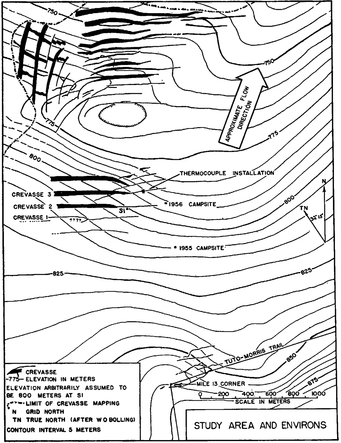
Fig. 1. Study area and environs

In the region under consideration there was definitely a line of incipient crevasse formation preceded by a considerable area undisturbed by crevasses, at least as manifested by any detectable surface fissures. The first three crevasses in the pattern were the subject of most of the studies by Meier’s party in 1955. Their location is shown on Figure 1. Crevasse No. 3 in particular was instrumented in detail, including all the thermocouples. It appears to start abruptly 102 m. west of the site of the thermocouple installation and gradually tapers out about 143 m. to the east. 92 m. west it intersects the east end of a large crevasse. At its point of origin at the west end it is about 2 m. in width at the surface and, on the average, exhibits this same width considerably to the east of the location of the thermocouples. Total depth of this latter location was estimated from tectonic, movement, and seismic data to be about 26 m. Instruments were actually installed to a depth of 19 m. It was Meier’s opinionReference Meier ¹ that the crevasse was about five years old in 1955.

At the instrument site the snow bridge over the crevasse remained intact throughout the 1955 summer. Personnel entered the crevasse through an opening cut in the snow bridge slightly to one side of the plane of instrumentation. An attempt was made to keep this opening closed by an artificial cover when not being used for personnel traffic. However, at the end of the 1955 season a hole about 2 ft. (0.61 m.) wide was left open briefly and was promptly covered with a natural bridge during a storm. The crevasse was entered again on 28 August 1956 and snow was found loosely banked against its south wall below a depth of 11 m. beneath the surface; apparently it was deposited during the storm at the end of the 1955 season. This obstruction was local, with the crevasse open to depths of approximately 18 m. to each side of the opening. The snow bridge thickness was 52 cm. on 13 August 1955. On 21 June 1956 measurements showed an accumulation of 115 cm. of snow during the winter.

Instrumentation

Between 30 July and 14 August 1955, 53 thermocouples were installed in a cross-sectional plane normal to the length of crevasse No. 3 (Fig. 1). The location of the thermocouples installed in and near the crevasse is shown in Figure 2. The coordinates of all the thermocouples are given in Table I. Not all of these instruments survived the 1955–56 winter. Specific details are given below:

Fig. 2. Location of thermocouples. 1956 surface. — — — — — 1955 surface. inactive in 1956

Table I. Thermocouple Coordinates for Crevasse Number 3, Blue Ice Valley

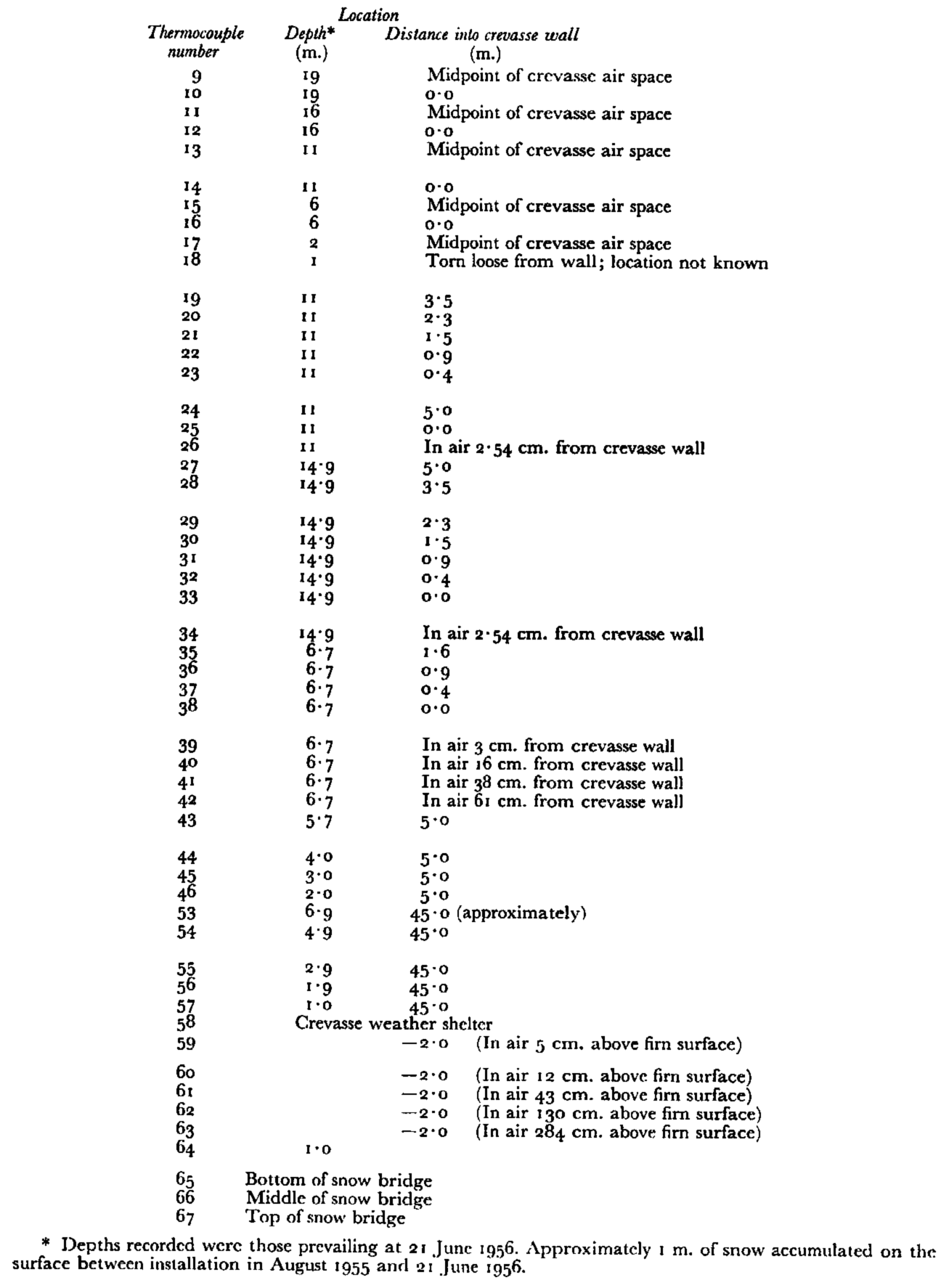
Thermocouples 9, 11, 13, 15 and 17. A string of thermocouples hanging vertically in the air space of the crevasse. Operative during the summer of 1955, but installation torn loose during winter.

Thermocouples 10, 12, 14, 16 and 18. All mounted on the face of the crevasse. No. 18 was torn loose from the wall shortly after installation and was not replaced. Leads from all were severed during winter.

Thermocouples 35, 36, 37 and 38. A horizontal traverse at a depth of 6.7 m. Holes drilled to a penetration of 1.6 m. with 1.25 in (3.2 cm.) ice drill. The string of thermocouple wires was slid in along the hole. The opening was then sealed with snow and ice but no attempt was made to pack the entire hole. The thermocouple junctions came to apparent thermal equilibrium in not more than one hour.

Thermocouples 19, 20, 21, 22, 23, 24, 25 and 26. A horizontal traverse at a depth of 11 m. Drilling and installation the same as with Nos. 35^–38.

Thermocouples 27, 28, 29, 30, 31, 32, 33 and 34. A horizontal traverse at a depth of 14.9 m.

Thermocouples 65, 66 and 67. A vertical traverse of the snow bridge, 65 at the bottom, 67 at the top, and 66 approximately at the mid-point. Leads severed during winter.

Thermocouples 43, 44, 45 and 46. A vertical traverse in the firn at a distance of 5 m. from the crevasse and reaching to a depth of 5.7 m. Hole drilled with 1.25 in. (3.2 cm.) ice drill. After placement of thermocouples, hole was rather loosely packed with ice and show. All thermocouples came to apparent thermal equilibrium in not more than one day.

Thermocouples 53, 54, 55, 56 and 57. A vertical traverse in the firn at a distance of approximately 45 m. from the crevasse reaching to a depth of 6.9 m. Apparently the walls of this test hole became water-wet during the drilling and remained so for some time after. During the period of observation in August 1955 all thermocouples in this hole indicated 0° C. (allowing for small systematic fluctuations). However, early in the summer of 1956, thermocouples in this hole yielded readings which appeared to indicate that they were in thermal equilibrium with the surrounding ice body. This hole was drilled with 4 in. (10.2 cm.) coring device. After placement of the thermocouple wires, the hole was rather loosely packed with snow and ice.

Thermocouples 39, 40, 41 and 42. A horizontal traverse in the air space at a depth of 6.7 m. in the crevasse. The thermocouples were positioned on a 1.125 in. (2.9 cm.) wooden dowel protruding horizontally from the face of the crevasse. Installation and leads were still intact in June 1956.

Thermocouples 59, 60, 61, 62, 63 and 64. A vertical traverse extending from the ice surface upward into the ambient air. Installation survived the winter but the leads were severed.

Thermocouple 58. A single thermocouple inside the crevasse weather shelter during August 1955. Location during summer 1956 not known.

The thermocouple wells in the sides of the crevasse were bored with a 1.25 in. (3.2 cm.) ice drill powered by a conventional 18 in. (45.7 cm.) carpenter’s hand brace. For the holes at 6.7 and 11 m. below the surface, the driller worked from a chair suspended from a hoist-works attached to a lightweight assault bridge; which had been positioned across the crevasse. Since the working space was very limited, every removal of the drill from the hole necessitated a disassembly of the tool. Because the drill clogged after a few inches of penetration, 87 breakdowns and reassemblies of the drill were required in order to bore a distance of 5 m. for the well 15 m. below the surface.

All the thermocouples consisted of copper–constantan junctions. A 20-gauge duplex, glass fiber insulated product supplied by Leeds and Northrup was used. The junctions and all necessary splices in the measurement circuits were made by means of commercial compression-type solderless fittings. These were particularly advantageous to install under the difficult work conditions. The solderless connectors were completely satisfactory during the summer of 1955. Some suspicion is cast on their long-term stability because of the failure of so many of the circuits during the winter. No attempt was made to isolate the point of failure. However, it is known that such compression connectors were blamed for the mechanical failure of wires under strain in several trail-marking installations.

A conventional electrical circuit was used for the measurement of the thermal electromotive force. For convenience of measurement, all leads were brought to one central instrument panel. The constantan side of all the thermocouples was used as an electrical common. The copper side of each junction was brought to a numbered hub of the instrument panel or to a numbered position on a 24-channel switch. A shortage of thermocouple wire in the field necessitated the use of copper wire of the lamp cord type for portions of the copper leads. Since the copper in the latter is presumably different from that in thermocouple wire, junctions between these two types of copper might give rise to a thermal electromotive force. However, a field experiment revealed that the magnitude of this effect was negligible with the instruments employed.

The thermometric electromotive force of the thermocouple junctions with respect to a reference junction at 0° C. was measured with a Rubicon portable potentiometer. This instrument was calibrated to read directly in ° C. for copper–constantan thermocouples. A precision of ±0.3° C. was reported by the manufacturer. The reference junction was maintained at 0° C. by immersion in a stirred air–water–ice mixture contained in a Dewar jar. The temperature of this reference mixture was checked periodically with a calibrated mercury-in-glass thermometer.

Measurements

The instrumentation described above was completed in 1955 only nine days before the project personnel left the ice sheet for the summer. Consequently, no transient data were obtained during the 1955 season. However, sufficient observations were made to define clearly the temperature distribution adjacent to the crevasse on 16 August 1955.

During the 1956 summer the thermocouples were read seven times in the interval 21 June to 28 August. These latter data and the 1955 data are tabulated in Table II exactly as recorded in the data books in the field. Apart from mistakes and systematic errors, the figures are believed reliable to 0.3° C. It will be seen in the next section that a few of the entries are obviously incompatible.

Table II. Thermal Data For Crevasse Number 3, Blue Ice Valley

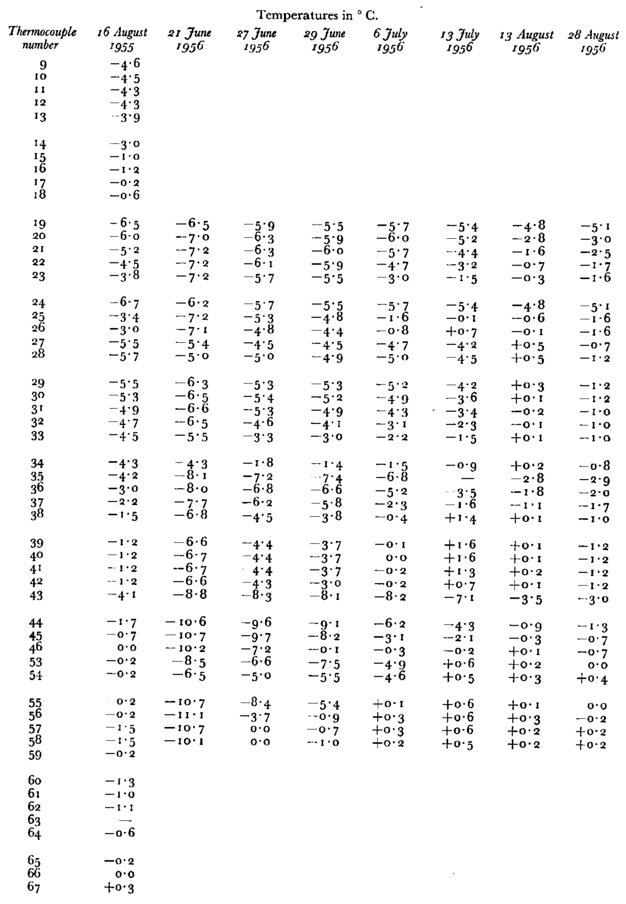
At the times when all of these measurements were made the surface of the glacier was essentially at 0° C. Diurnal temperature fluctuations would have had little effect on the temperature distributions except very near the surface. Although it would be interesting to correlate the reported temperature distributions with the seasonal variation of the mean daily temperatures, the intermittent occupation of this study area made it impossible to obtain these latter data. Temperature profiles in the undisturbed glacier indicate a mean annual temperature of −12° C. in this area.

Analysis of the Data

The temperature distribution in and adjacent to the crevasse is shown for each of eight different times in Figures 3 to 10. The isotherms in these figures were drawn in by process of repeated smoothing of the raw data. Isotherms were sketched crudely first on a series of large−scale work plots, one for each time listed in Table II. For each of 12 of the thermocouple locations, plots of temperature vs. time were prepared. Sharp corners and erratic fluctuations on these graphs were replaced by smooth curves. These smoothed values of temperature were transferred back to Figures 3 to 10, making small changes where necessary in the position of the isotherms. This process was continued until the resulting temperature distribution was smooth with respect to both time and spacial variation. Consequently, the isotherms drawn in Figures 3 to 10 represent a certain amount of subjective engineering interpretation.

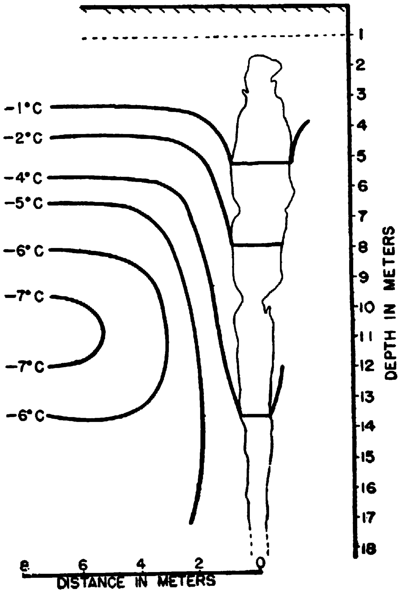
Fig. 3. Temperature distribution on 16 August 1955

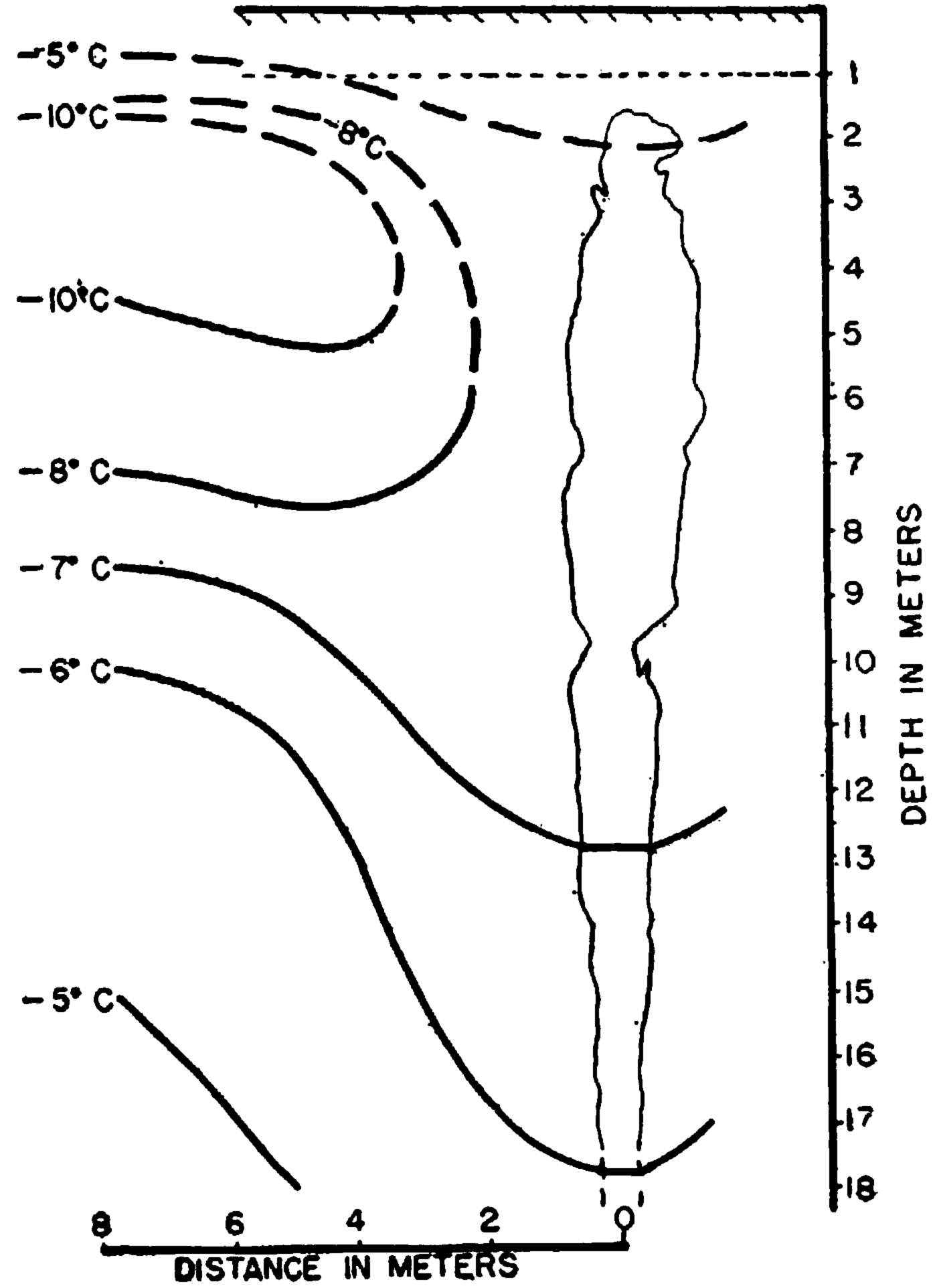
Fig. 4. Temperature distribution on 21 June 1956

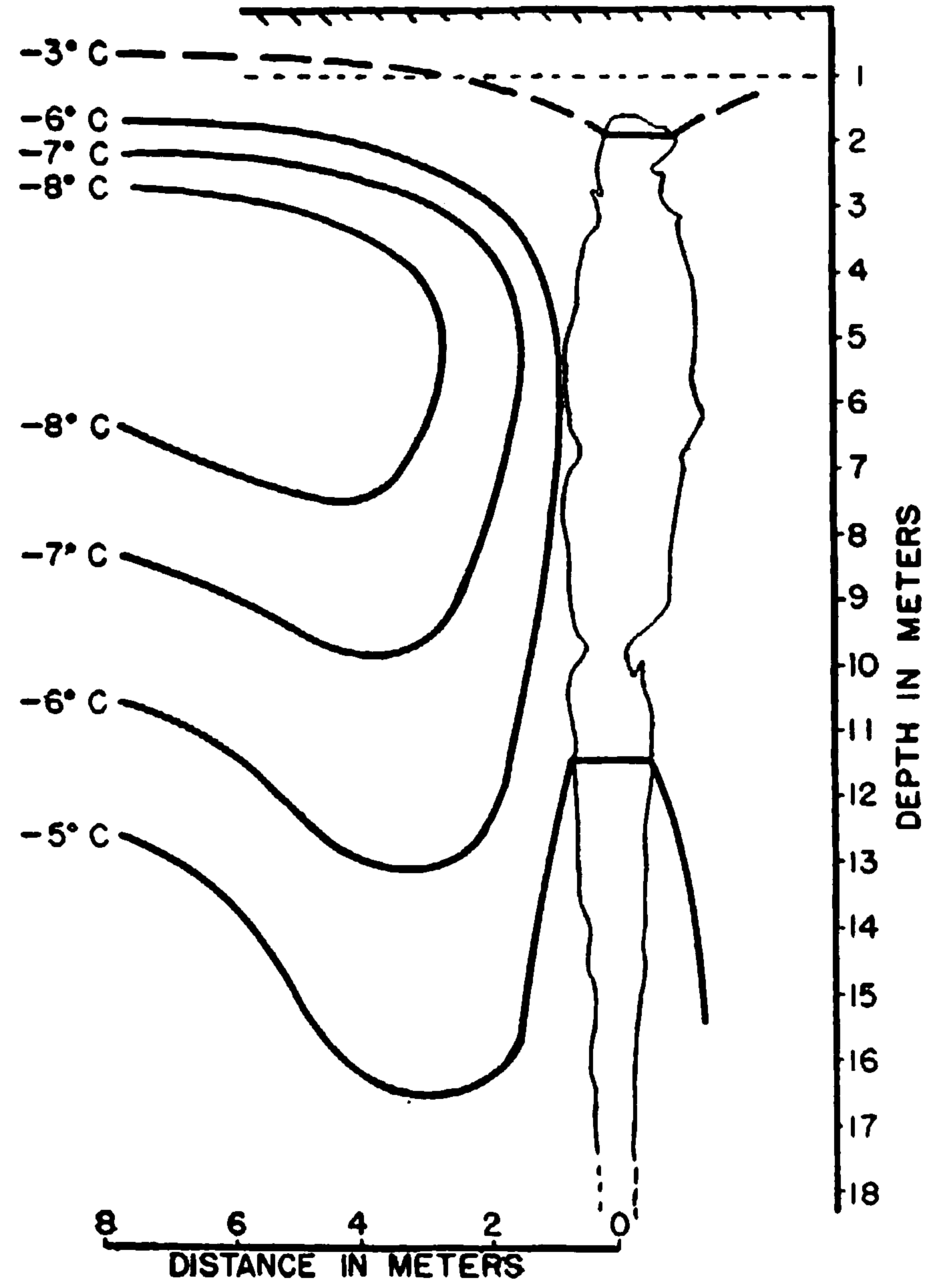
Fig. 5. Temperature distribution on 27 June 1956

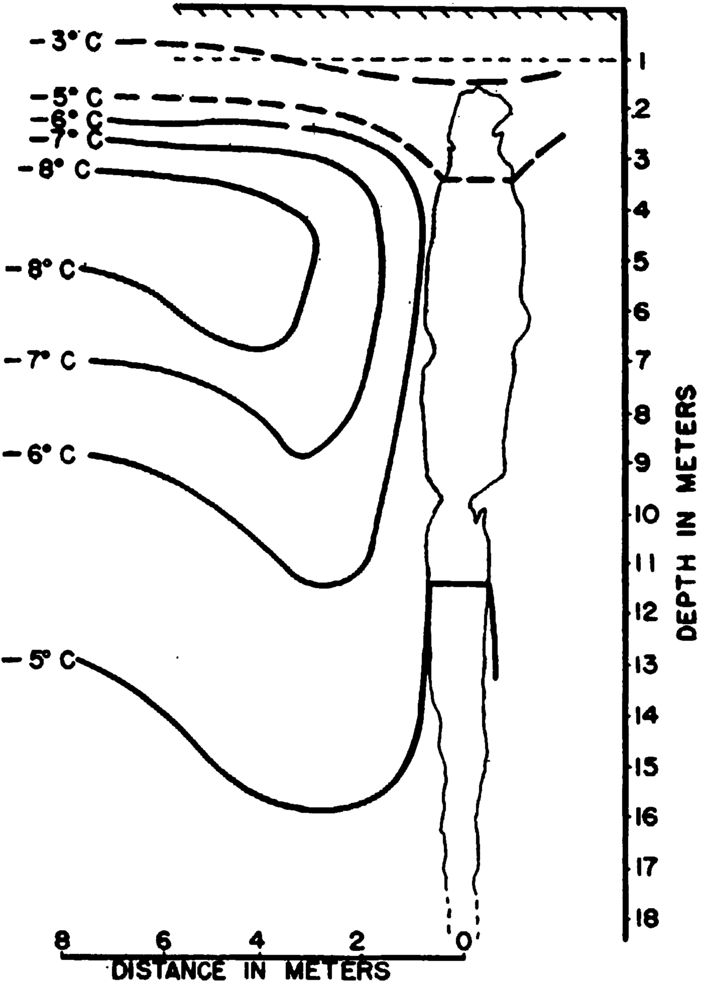
Fig. 6. Temperature distribution on 29 June 1956

Fig. 7. Temperature distribution on 6 July 1956

Fig. 8. Temperature distribution on 13 July 1956

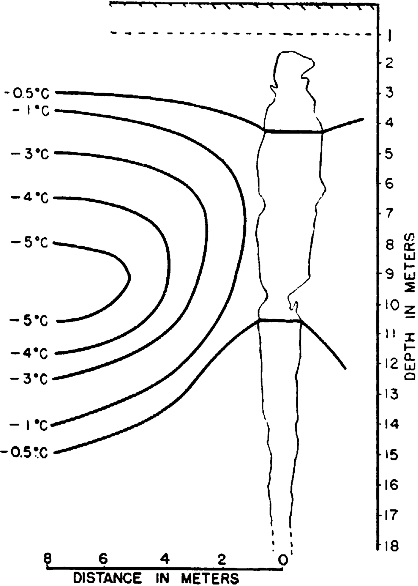
Fig. 9. Temperature distribution on 13 August 1956

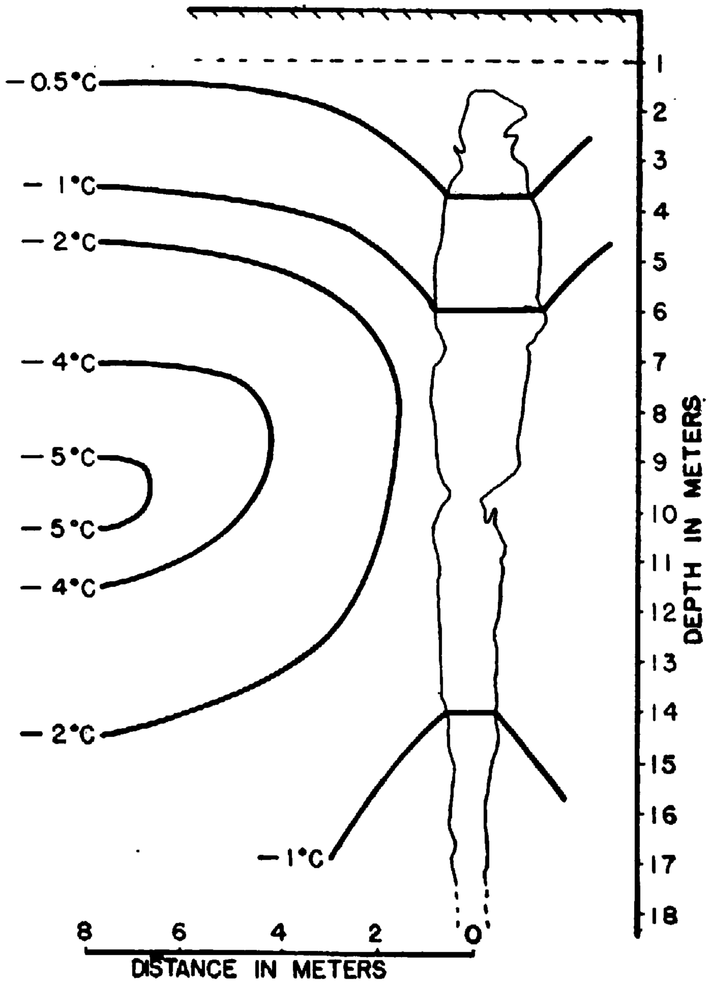
Fig. 10. Temperature distribution on 28 August 1956

The time variations of the locations of the −1, −4, −5, −7 and −8° C. isotherms are shown in Figures 11 to 15. These figures probably indicate most clearly the transient thermal history of the area adjacent to the crevasse during the 1956 summer thaw.

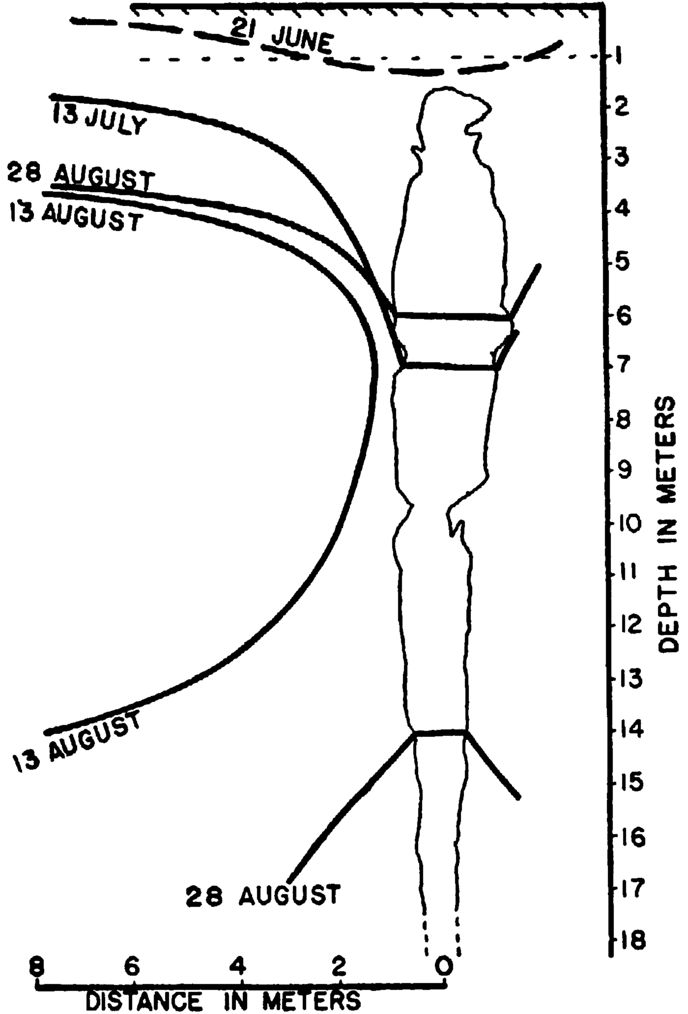
Fig. 11. Time variations of the location of −1° C. isotherm during 1956

Fig. 12. Time variations of the location of −4° C. isotherm during 1956

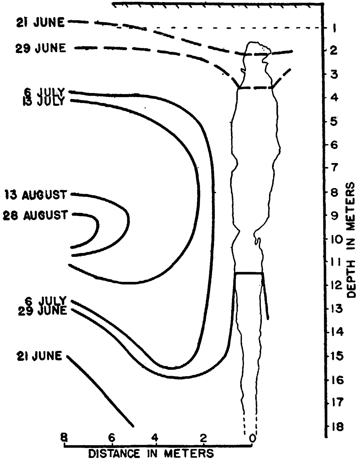
Fig. 13. Time variations of the location of −5° C. isotherm during 1956

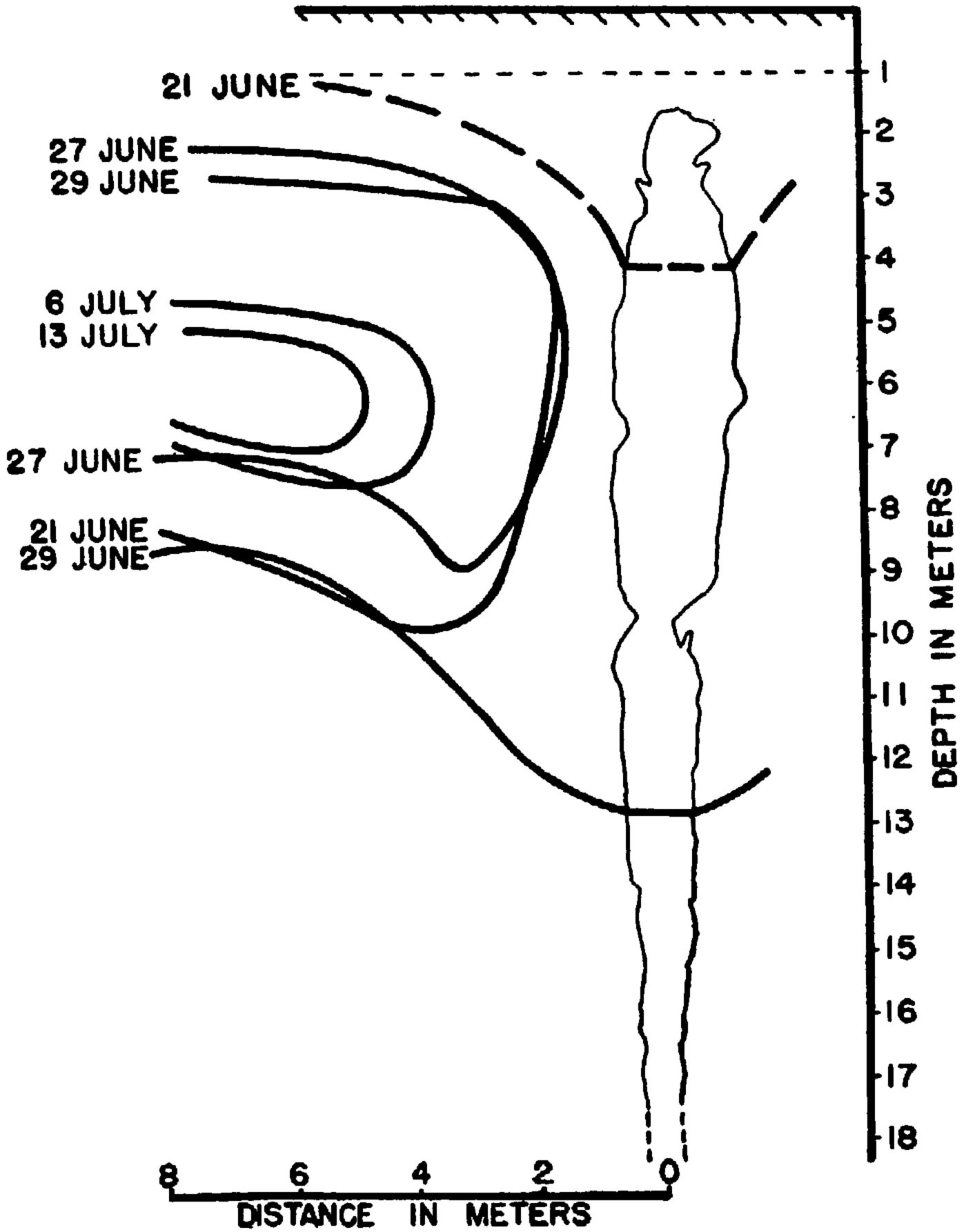
Fig. 14. Time variations of the location of −7° C. isotherm during 1956

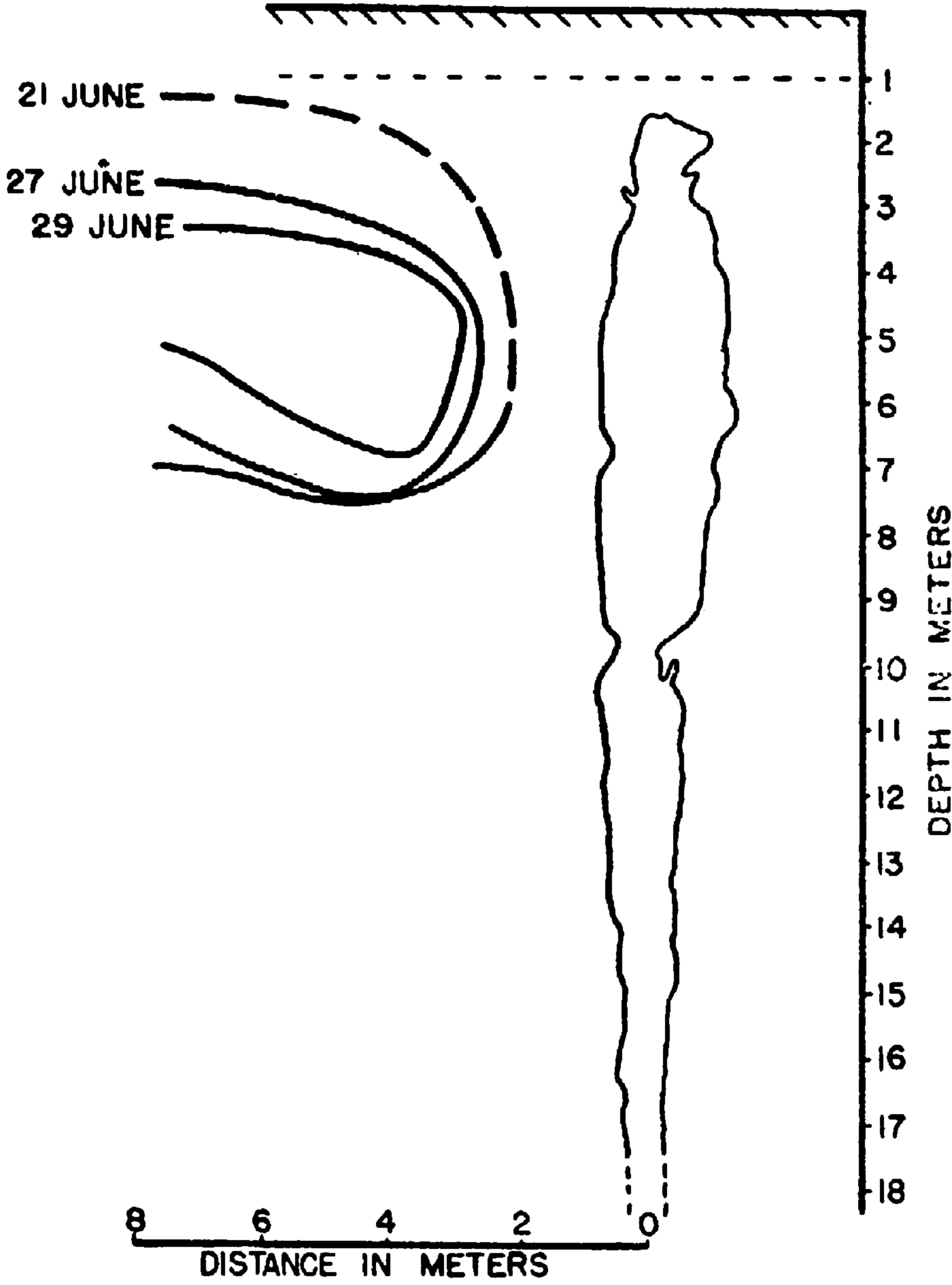
Fig. 15. Time variations of the location of −8° C. isotherm during 1956

Heat Flux in the Vicinity of a Crevasse

The temperature data portrayed in Figure 3 were used to estimate the heat flux distribution in the vicinity of the crevasse. A family of flux lines was sketched orthogonal to the isotherms as shown in Figure 16. The flux lines were all started outward from the −7° C. isotherm equally spaced along that isotherm. Interpretation of the temperature data within the crevasse air space is somewhat difficult. Heat transfer due to convection and mass transfer is probably significant. Therefore, it was assumed that all heat entering the crevasse wall either came through the snow bridge directly above the crevasse or from geothermal sources directly below the crevasse. Flux lines intersecting the crevasse wall were therefore turned vertically upward or vertically downward as indicated in Figure 16. The methods employed in arriving at this flux distribution are somewhat less than elegant. Considerable refinement would be necessary in order to attach quantitative significance to the results. However, the distribution obtained does give positive qualitative indication of an appreciable flux peak above the crevasse snow bridge. This is apparently compatible with preliminary observations made with thermal flux and radiation type crevasse detectors.Reference Hansen ³

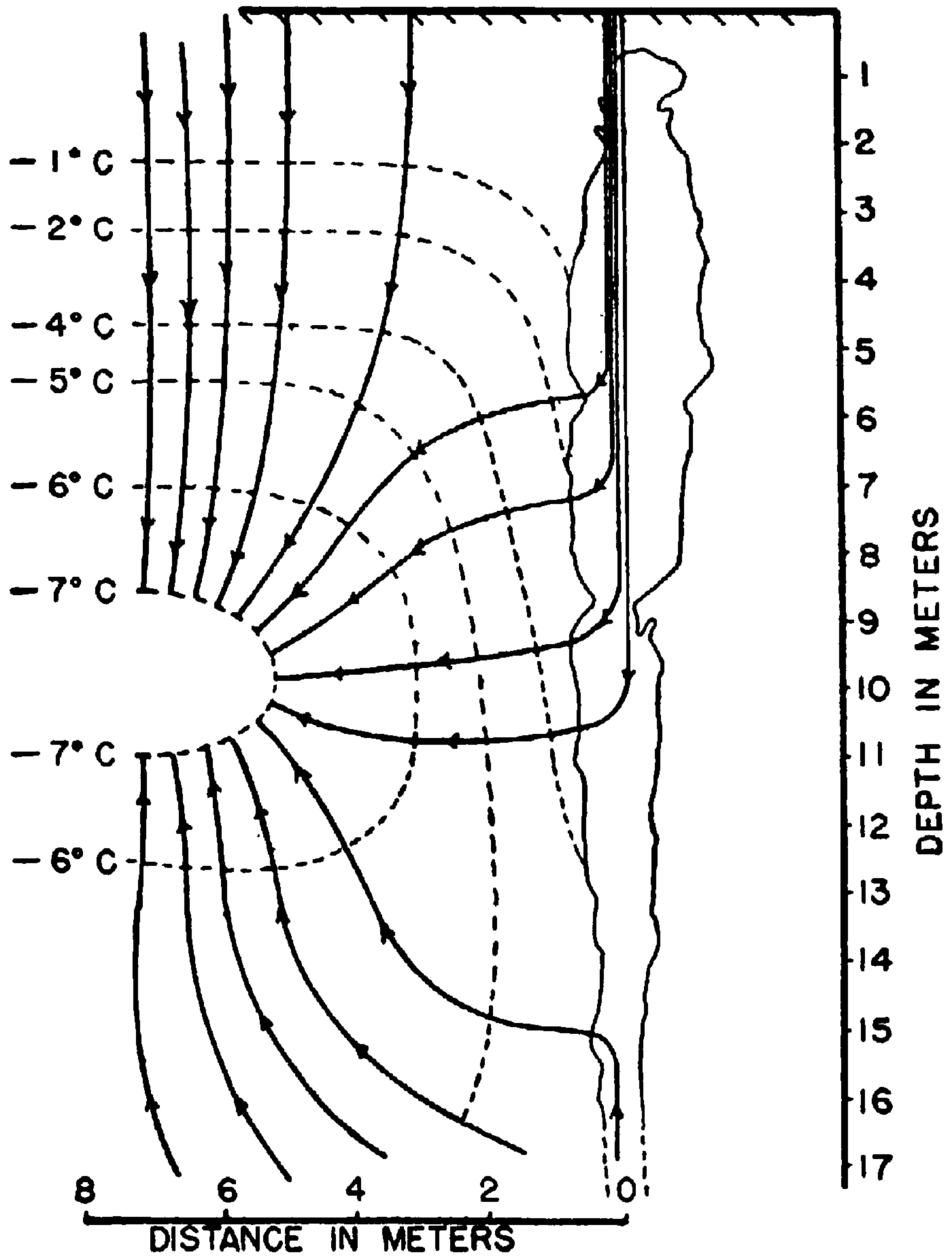
Fig. 16. Heat flux distribution on 16 August 1955