


1. Introduction
Fine control over plasma parameters is beneficial for experiments that use destructive diagnostics (Hurst et al. Reference Hurst, Danielson, Dubin and Surko2016; Ahmadi et al. Reference Ahmadi, Alves, Baker, Bertsche, Butler, Capra, Carruth, Cesar, Charlton and Cohen2017; Stenson et al. Reference Stenson, Nißl, Hergenhahn, Horn-Stanja, Singer, Saitoh, Pedersen, Danielson, Stoneking and Dickmann2018), have long cycle times (Amsler et al. Reference Amsler, Antonello, Belov, Bonomi, Brusa, Caccia, Camper, Caravita, Castelli and Cheinet2021; Singer et al. Reference Singer, König, Stoneking, Steinbrunner, Danielson, Schweikhard and Pedersen2021; Blumer et al. Reference Blumer, Charlton, Chung, Clade, Comini, Crivelli, Dalkarov, Debu, Dodd and Douillet2022) or struggle for limited resources like antimatter (Hori & Walz Reference Hori and Walz2013), rare isotopes (Aumann et al. Reference Aumann, Bartmann, Boine-Frankenheim, Bouvard, Broche, Butin, Calvet, Carbonell, Chiggiato and De Gersem2022) or highly charged ions (Kluge et al. Reference Kluge, Beier, Blaum, Dahl, Eliseev, Herfurth, Hofmann, Kester, Koszudowski and Kozhuharov2008). For many of these experiments, the density $n$ and temperature $T$
 of the plasma are key parameters which must be both reproducible, for the reasons just stated, and optimal. In practice, the maximum $n$
 and minimum $T$
 are far from the theoretical optimum, and it remains an open question whether the observed bounds on $n$
 and $T$
 are fundamental or merely a sign that better methods are required.
For an electron or positron plasma, $n$ can be continuously tuned using the strong drive regime (SDR) rotating wall technique of Danielson, Surko & O'Neil (Reference Danielson, Surko and O'Neil2007). The value of $T$
 may be reduced via evaporative cooling (EVC) (Andresen et al. Reference Andresen, Ashkezari, Baquero-Ruiz, Bertsche, Bowe, Butler, Cesar, Chapman, Charlton and Fajans2010). When the plasma is cold enough that $T$
 is less than its space charge $\phi _0$
 ($k_B T \ll e\phi _0$
 , where $k_B$
 is Boltzmann's constant and $e$
 is the elementary charge), then EVC also reliably defines the latter. Combining these two tools yields a new one, SDREVC, which allows $n$
 , $\phi _0$
 , and $T$
 to be set simultaneously (Ahmadi et al. Reference Ahmadi, Alves, Baker, Bertsche, Capra, Carruth, Cesar, Charlton, Cohen and Collister2018).
When it works, SDREVC takes as input ‘any’ plasma (of sufficiently many particles) and produces a user-defined, invariable (to ${\sim }1\,\%$ ) final state – greatly facilitating optimization studies and systematic searches generally. But when does it work? A priori, the experimenter cannot give an exhaustive list of the conditions necessary for these techniques to work as advertised. The main ingredient (SDR) is only heuristically described by theory. One must be content to find, empirically, some range of parameters which give good results for a particular trap.
It is useful to know what limits exist and which assumptions are actually relevant to the process. We explore these questions in experiments on electron plasma held in ASACUSA's Cusp Trap (Kuroda et al. Reference Kuroda, Tajima, Radics, Dupré, Nagata, Kaga, Kanai, Leali, Rizzini and Mascagna2017). Section 2 reviews aspects of the control and diagnostic systems relevant for this work. Each technique is addressed in its own section: SDR in § 3, SDREVC in § 4 and EVC in § 5. Section 6 contains a short discussion of the results, summarizing what can be used for testing a potential theory, and indicating where practical extensions may be possible.
2. Apparatus
We use a Penning Malmberg trap (Malmberg & Driscoll Reference Malmberg and Driscoll1980) with inner diameter $34\ \mathrm {mm}$ and magnetic field $B\approx 2\ \mathrm {T}$
 . The entrance and exit to the trap are screened by copper meshes (geometrical transparency = $79\,\%$
 ) so that microwave radiation from the plasma cannot escape the $6\ \mathrm {K}$
 cryogenic ultra-high vacuum region (Amsler et al. Reference Amsler, Breuker, Chesnevskaya, Costantini, Ferragut, Giammarchi, Gligorova, Gosta, Higaki and Hunter2022). A typical plasma contains $N\sim 10^7$
 electrons, with length $L_p\approx 10\ \mathrm {cm}$
 , radius $r_p\approx 1\ \mathrm {mm}$
 and $n\sim 10^8\ \mathrm {cm}^{-3}$
 . The plasma cools via cyclotron radiation to a steady-state $T\approx 30\ \mathrm {K}$
 for $N\lesssim 4 \times 10^7$
 .
.
2.1. Control
Two pairs of superconducting anti-Helmholtz coils produce $B$ . The axial component of $B$
 is shown in figure 1(a). The strong gradients were designed to focus low field seeking antiatoms travelling to the right toward the spectroscopy beamline (Nagata & Yamazaki Reference Nagata and Yamazaki2014; Nagata et al. Reference Nagata, Kanai, Kuroda, Higaki, Matsuda and Yamazaki2015). Although the coils produce a strong field in three regions, it is difficult to move a plasma into the middle or right region because of the field nulls (cusp points) at ${\pm }120\ \mathrm {mm}$
 . Plasma is loaded exclusively on the left side, either from an electron source (Nishinbo NJK1120A) or from other traps. Plasma diagnostics (see below) are also performed by dumping to the left.
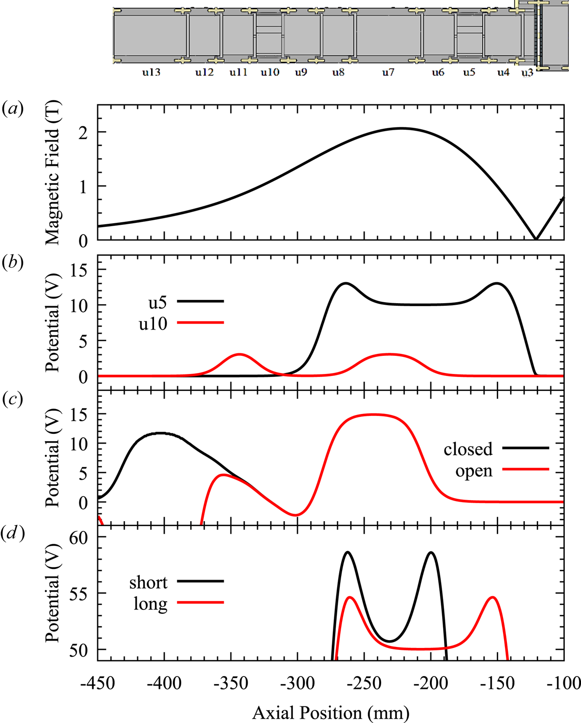
Figure 1. Electrode structure and on-axis trapping fields. Two-dimensional rendering of the electrode stack (with electrode names) is shown at the top, followed by (a) magnetic field strength $B$ and electrostatic potential for (b) standard SDREVC, (c) pulsed SDREVC and (d) EVC. In this figure the voltages are multiplied by ($-$
 1) for clarity; they must be inverted for confining negatively charged particles.
One electrode, u13, must be pulsed for catching bunches of protons, antiprotons and positrons from those traps (electrode locations are given at the top of figure 1). Two electrodes, u5 and u10, are driven with radiofrequency for SDR and plasma or ion heating. The other electrodes (u12, u11, u9, u8, u7, u6, u4, u3) have cryogenic 2-pole RC filters mounted as close to the electrode as possible (${\sim }1 \mathrm {cm}$ away). These filters attenuate noise with frequency $f>10\ \mathrm {kHz}$
 , which would heat the plasma. The pulsed electrode u13 has a similar filter, but the filter is bypassed by a pair of BAT54 Schottky diodes. The slower, nearly DC bias for the electrodes is supplied by low speed x15 high voltage amplifiers designed by J. Fajans. These amplifiers exhibit excellent stability (approximately $1\ \mathrm {mV}$
 per year) and noise performance ($0.1 \mathrm {mV_{\rm rms}}$
 ). The price for this performance is a rise time of almost $5 \mathrm {ms}$
 . This limits the range of plasma dynamics which can be studied in our experiment; for instance, after EVC we must spend $10 \mathrm {ms}$
 changing the well shape before we can properly diagnose $T$
 .
.
The rotating wall (RW) electrodes u5 and u10 have 4 azimuthal sectors each. Each sector is driven with a sine wave, phase shifted as $\{0^\circ, 90^\circ, 180^\circ, 270^\circ \}$ . These signals are produced by the $\{0^\circ, 90^\circ \}$
 outputs of a 2-channel arbitrary waveform generator (BK Precision BK4054B) followed by $180^\circ$
 phase splitters (Mini-Circuits ZSCJ-2-2+). The signals then enter a filterbox mounted to the vacuum feedthrough. The filterbox contains a low pass filter for DC biasing of the electrode (${\rm RC}=0.2\ \mathrm {ms}$
 ) and high pass filters for the RW signals (${\rm RC}= 0.01\ \mathrm {ms}$
 ).
).
One sector of u10 is grounded inside the vacuum chamber (unintentionally); the resistance to ground is less than $4\Omega$ and does not change when the experiment is cooled down. The filter for u10 was modified such that a DC bias could still be applied to two opposing sectors, while the others are $50\Omega$
 terminated. A DC bias is applied when dumping the plasma so that the particles leave the trap with at least $10\ \mathrm {eV}$
 of energy. The bias creates an azimuthal asymmetry, which leads to more rapid plasma expansion (Notte & Fajans Reference Notte and Fajans1994). This effect is negligible for short manipulations ($10\ \mathrm {ms}$
 or less). The AC inputs to u10 are essentially the same as for u5's filter. In both cases, the impedance between RW sectors is approximately $50\Omega$
 at frequencies above $f \sim 10\ \mathrm {kHz}$
 .
.
A high voltage pulser drives electrode u13 via a similar filter circuit with ${\rm RC}=0.2\ \mathrm {ms}$ . The pulser is similar to the one described by Chaney & Sundararajan (Reference Chaney and Sundararajan2004), with the addition of a transformer and relay to produce pulses of either polarity.
2.2. Diagnostics
To measure the plasma parameters $T$ , $r_p$
 and $N$
 , we must dump the plasma out of the trap against a microchannel plate-phosphor screen detector (MCP) (Peurrung & Fajans Reference Peurrung and Fajans1993). Since this operation destroys the plasma, only one of its properties is measured. Cycle-to-cycle reproducibility is therefore a basic assumption in this work. Using SDREVC we achieve ${\rm d}N/N<1\,\%$
 for any desired initial state.
To get $T$ , the plasma is released slowly (${\sim }1\ \mathrm {ms}$
 ). The flux of escaping particles is amplified by the MCP and generates a light signal on the phosphor screen. This signal, measured by a SiPM, is combined with the time-dependent confinement potential to reconstruct the tail of a Maxwellian (Eggleston et al. Reference Eggleston, Driscoll, Beck, Hyatt and Malmberg1992). On a graph of $\mathsf {log}\mathrm {[SiPM\ signal]}$
 vs. $\mathrm {-[confinement]}$
 , the slope of the line that fits the rising edge is $e/k_BT$
 .
.
To get $r_p$ or $N$
 , the plasma is released quickly (${\sim }1\ \mathrm {\mu }$
 s) using the high voltage pulser described above. The radial profile is captured by a CMOS camera (Thorlabs CS165MU1) and fit to a modified Gaussian (Evans Reference Evans2016). To measure $N$
 , the back of the MCP is grounded, while the front (biased at $+10\ \mathrm {V}$
 ) is connected to an integrator which produces a voltage $V=GNe/C$
 , where $G=168$
 is the amplifier gain and $C=1.09\ \mathrm {nF}$
 is the combined capacitance of amplifier, cabling and parasitics.
The parameters $L_p$ and $n$
 can be derived from $r_p$
 , $N$
, $N$ and the confining potentials. There exist several numerical plasma solvers for precise estimation of these quantities, but most of them assume that $B$
 is uniform; see for example Peinetti et al. (Reference Peinetti, Peano, Coppa and Wurtele2006). Instead of developing a new code, here, we simply compute $n\approx N/{\rm \pi} r_p^2 L_p$
 , where $n$
 and $r_p$
 , which actually vary with $B$
 , are understood to be an average over the length. In the limit $kT\ll e\phi _0$
 , $L_p$
 can be estimated as follows. We slowly release the plasma and record the on-axis potential difference between well bottom and barrier when the first particles begin to escape. This potential difference is approximately $\phi _0$
 at that instant. At the same instant, $L_p$
 is approximately the distance between the turning points of barely confined particles. To get from this to the plasma length during RW compression, we note that the product of $L_p$
 and $\phi _0$
 is roughly constant, i.e. $\phi _0 \propto N/L_p$
 for a long plasma. The length of the fully confined plasma is then chosen from a table of $L_p$
 vs. $\phi _0 \times L_p$
 for the appropriate well.
3. SDR
The RW technique is used to control $r_p$ , and hence $n$
 (Huang et al. Reference Huang, Anderegg, Hollmann, Driscoll and O'neil1997). An electric dipole field with an amplitude of order $1 \mathrm {V}\ \mathrm {cm}^{-1}$
 revolves around the plasma in the plane perpendicular to $B$
 . The field presumably perturbs the radial edge of the plasma; it may also cause the centre of mass to oscillate (there is some speculation that the RW can recentre a plasma which began on a small diocotron orbit (A. P. Povilus, private communication 2014)). In the SDR, $n$
 evolves until the natural rotation rate of the plasma matches the RW frequency $f$
 (Danielson & Surko Reference Danielson and Surko2006).
In this regime, a graph of $n$ vs. applied frequency $f$
 should be a line starting from the origin with slope $n/f=4{\rm \pi} \epsilon _0 B/e$
 , where $\epsilon _0$
 is the permittivity of free space (Ahmadi et al. Reference Ahmadi, Alves, Baker, Bertsche, Capra, Carruth, Cesar, Charlton, Cohen and Collister2018). Practically, we search for some combination of on-axis potential, RW amplitude and RW frequencies such that the linear relation is observed for the widest range of frequencies possible. Figure 2 shows examples from our experiment. The data are obtained by first preparing $13\times 10^6$
 or $28\times 10^6$
 electrons via SDREVC at $200\ \mathrm {kHz}$
 in u5 (see figure 1b), then moving to another SDR well and compressing for $10\ \mathrm {s}$
 at a different frequency $f$
 and higher RW amplitude (the RW waveforms are about $4\ \mathrm {V_{pp}}$
 at the vacuum feedthrough). The SDR wells ‘u5’ and ‘u10’ are similar to those shown in figure 1(b).
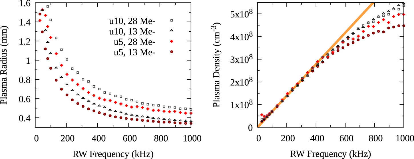
Figure 2. Control of the plasma density $n$ using SDR in u5 and u10, for $N=13\times 10^6$
 or $N=28\times 10^6$
 . Left: plasma radius $r_p$
 , measured as a function of applied RW frequency. Right: plasma density, evaluated as $n=N/({\rm \pi} r_p^2 L_p)$
 .
.
Compression in u5 is linear up to approximately $400 \mathrm {kHz}$ ; for u10 the range is slightly higher. In general, the useful range of SDR is less than $1\ \mathrm {MHz}$
 for our experiment. A similar limit was found by Ahmadi et al. (Reference Ahmadi, Alves, Baker, Bertsche, Capra, Carruth, Cesar, Charlton, Cohen and Collister2018). Danielson et al. (Reference Danielson, Surko and O'Neil2007) suggested that SDR fails when the rotation rate is too close to one of the plasma's Trivelpiece–Gould modes, and that a stronger drive or a higher frequency can recover SDR in this case. However, we do not recover SDR for any frequency above $400\ \mathrm {kHz}$
 . (Higher RW amplitude cannot be tested, but we do find that the amplitude can be decreased by a factor of 4 in u10 without changing the resulting radii.) We find that the steady-state $T$
 (while RW is still applied) increases monotonically with higher RW frequency, from $200\ \mathrm {K}$
 at $500 \mathrm {kHz}$
 to over $20\ 000\ \mathrm {K}$
 at $3 \mathrm {MHz}$
 . This may be a sign of increased expansion heating, which is expected at higher $n$
 , or else a symptom of phase slip between the drive and the plasma. A high-$T$
 failure mode would have been less relevant for Danielson et al. (Reference Danielson, Surko and O'Neil2007), where $B=4.8\ \mathrm {T}$
 , implying at least ten times faster cyclotron cooling in that experiment than in ours.
Within the range of frequencies where $n$ is linear in $f$
 , we measure the same $n$
 for both test values $N=13\times 10^6$
 and $N=28\times 10^6$
 . Accordingly, for higher $N$
 , $r_p$
 (and $L_p$
 ) is relatively greater, while for greater $L_p$
 (u5 vs. u10), $r_p$
 is relatively smaller. These trends are clear from the data in figure 2. Thus, the data confirm our expectations for SDR compression. We conclude that the factor of two mirror field ratio does not compromise SDR in u5 or u10, nor does the use of a RW perturbation generated by three out of four $90^{\circ }$
 azimuthal sectors. No particles are lost, no halo is produced, no diocotron is induced and $T$
 is low ($100\unicode{x2013}200\ \mathrm {K}$
 ) in both wells over the linear (SDR) range of RW frequencies.
We note, however, that our results do not reproduce the $B$ dependence expected from the relation $n/f=4{\rm \pi} \epsilon _0 B/e$
 . First, the line in figure 2 has a slope corresponding to $B=1\ \mathrm {T}$
 , which is a field value only reached at one extremity of the plasma; everywhere else the field is higher. Second, a given frequency should presumably give a denser plasma in u5 than in u10, because the average $B$
 in u10 is lower: $\langle B\rangle =1.35\ \mathrm {T}$
 in u10 and $1.87 \mathrm {T}$
 in u5. Yet the graph of $n \mathrm {vs.}\ f$
 is nearly the same for both wells. The analysis may be compromised by other effects arising from the strong mirror field in the Cusp trap. A plasma spanning a large range of $B$
 should still reach a rigid-rotor equilibrium defined by a single rotation rate, but it is by no means cylindrical (Fajans Reference Fajans2003). A simple axial average $\langle B\rangle$
 does not reflect the true distribution of particles, partly because of magnetic mirroring. Moreover, the assumption that particles follow the field lines does not hold for non-neutral plasma equilibrium in a magnetic mirror. This latter effect would tend to make the u5 plasma expand more than the u10 plasma during transfer to the pulsed dump well used for imaging, albeit only by a factor of $5\,\%$
 if we use the first approximation given by Fajans (Reference Fajans2003).
4. SDREVC
Starting with sufficiently many particles in any initial state, we use SDR to control $n$ and EVC to control $\phi _0$
 (Ahmadi et al. Reference Ahmadi, Alves, Baker, Bertsche, Capra, Carruth, Cesar, Charlton, Cohen and Collister2018). Since $n$
 and $\phi _0$
 completely define the cold plasma equilibrium for a given well shape, this operation also fixes the remaining parameters $L_p$
 , $r_p$
 and $N$
 . In this section, we will first show that SDREVC, like SDR, works as well in u5 as in u10, with its strong gradient and one grounded RW sector. We then demonstrate a different, pulsed protocol, whereby $\phi _0$
 is reduced without EVC, resulting in the same level of reproducibility as standard SDREVC.
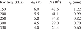
For this section we define ‘any initial state’ to be any one of five starting points prepared using SDREVC in u5. That is, we begin with SDREVC with the parameters given in one of the rows of table 1. Then we change wells, frequency and protocol for the final SDREVC to a fixed value.
Table 1. Set of initial plasma preparations for testing different SDREVC routines.
4.1. Standard Protocol
We implement SDREVC by starting in an SDR well and slowly reducing the confinement. In order to maintain a constant amount of overlap with the RW electrode as the space charge decreases, we reduce both sides of the confining potential simultaneously. The starting point of this operation is shown in figure 1(b) for wells in u5 and u10. The excess charge is slowly released (EVC for $18\ \mathrm {s}$ ) while $n$
 is locked by SDR at $200\ \mathrm {kHz}$
 .
.
The final number of electrons is plotted in figure 3 (left panel). Slightly different endpoints ($N=17.9$ and $19.4\times 10^6$
 ) were chosen for the different SDREVC protocols so that the data would not overlap. The deviation from the endpoint value, as well as the standard deviation, is $1\,\%$
 or less for any initial condition ($1\,\%$
 is one minor tick in the figure).
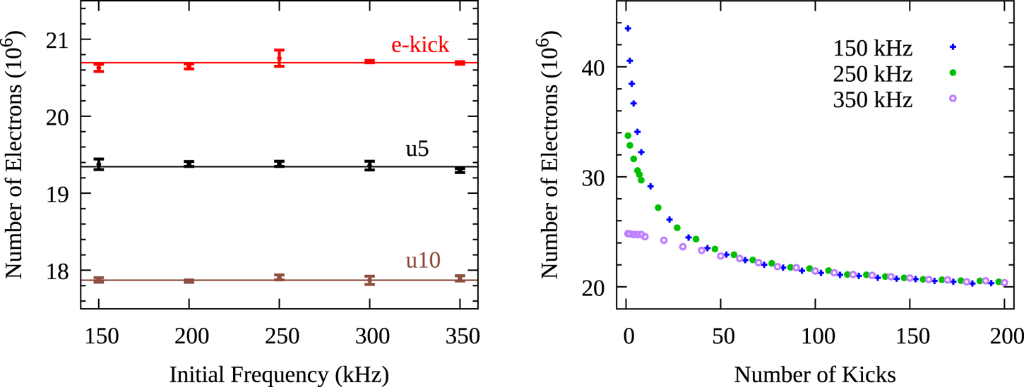
Figure 3. Control of the number of electrons using SDREVC and a variant with EVC replaced by e-kick. Left panel: reproducibilityof final number of electrons after SDREVC in u5 or u10 or the e-kick variant, for different initial plasma preparations (see table 1); data are reported as the mean of four measurements, with error bars showing ${\pm }1$ standard deviation. Right panel: convergence of the e-kick routine for three of these preparations; data points represent single measurements. The average number of electrons reported for the e-kick data set on the left is slightly higher (${\rm mean}=20.7$
 instead of 20.4) than the endpoint of the data on the right due to an unintended difference in the dump protocol (65 V instead of 100 V dump pulse).
4.2. Pulsed Protocol
Instead of slowly reducing the confinement, we may use the pulsed electrode u13 to rapidly open and close the well such that only a fraction of the particles have time to escape. Such pulsing is sometimes referred to as an e-kick because electrons are thereby ‘kicked out of’ a mixed electron–antiproton plasma without losing the antiprotons. We use a $65\ \mathrm {V}$ , $50 \mathrm {ns}$
 high voltage pulse to briefly switch from the ‘closed’ to ‘open’ configurations shown in figure 1(c). This is done once every $100\ \mathrm {ms}$
 , which means the plasma is in the ‘closed’ well for $99.9999\,\%$
 of the operation.
The routines used to obtain the data in the left panel of figure 3 employ 200 e-kicks, which amounts to $20 \mathrm {s}$ of RW compression and pulsing. The right panel shows the evolution of $N$
 as the number of e-kicks is varied. The convergence of different initial conditions to a common (exponential) curve is faster than the exponential convergence of the entire set to a final, minimum value of $N$
 .
.
Immediately after turning off the RW, we measure $T=170\ \mathrm {K}$ for standard SDREVC in u5, $130\ \mathrm {K}$
 for the same in u10, and $400 \mathrm {K}$
 for the pulsed protocol. Not surprisingly, the e-kicked plasma is hotter. The ramp-shaped well shown in figure 1(c) gives better results with fewer e-kicks than a flat well. We assume this is either because the average $B$
 is higher (more cooling) than for a flat well spanning the same range in the axial direction, or because the ramp pushes the bulk of the plasma away from the high voltage pulses applied to u13 (less heating). Compression in the ramp-shaped well is not quite SDR; the graph of $n \mathrm {vs.}\ f$
 is linear up to approximately $400 \mathrm {kHz}$
 , but the intercept is slightly above the origin. This may also contribute to plasma heating. The high level of reproducibility obtained with the pulsed protocol is remarkable, given these apparent disadvantages.
5. EVC
Once the plasma has cooled to a low steady-state $T$ , EVC is often used to reduce $T$
 further. However, forced EVC does not always lower $T$
 . In this section, we present data which suggest a link between $\phi _0$
 and the ultimate $T$
 achievable using EVC.
Figure 4 plots $T$ as a function of $\phi _0$
 for plasma with the initial parameters given in the caption. The plasma is prepared with SDREVC, allowed to cool with the RW off for $10\ \mathrm {s}$
 and then evaporatively cooled by reducing the confinement over $300 \mathrm {ms}$
 . Different choices of final voltage on the rightmost potential barrier result in different final values of $\phi _0$
 and $T$
 . In this figure, data points and error bars represent the mean and standard deviation of 4 measurements; outliers were removed by starting with 5 measurements per bin and removing the one that deviated the most. ‘Long’ and ‘short’ refer to the well shapes shown in figure 1(d). The well bottom is at $50\ \mathrm {V}$
 to improve the signal for the temperature diagnostic, which follows with as little manipulation as possible after EVC.
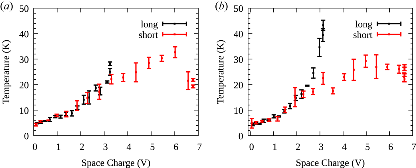
Figure 4. Evaporative cooling of electrons prepared with SDREVC at $150\ \mathrm {kHz}$ (a) or $350\ \mathrm {kHz}$
 (b). Initial plasma parameters (rightmost points of each dataset) are $N=19\times 10^6$
 , $r_p=0.72 \mathrm {mm}$
 (a) and $N=16\times 10^6$
 , $r_p=0.45\ \mathrm {mm}$
 (b). The initial $T$
 is somewhat higher for the denser plasma in the long well.
For $\phi _0>3\ \mathrm {V}$ , EVC does not reduce $T$
 . For $\phi _0<3\ \mathrm {V}$
 , $T$
, $T$ is completely determined by the final value of $\phi _0$
 . For example, if we want to EVC to $T<15\ \mathrm {K}$
 , we must have $\phi _0<2 \mathrm {V}$
 . The value $\phi _0=2\ \mathrm {V}$
 corresponds to a range $4.5< N<15\times 10^6$
 and $0.3< n<1.2\times 10^8\ \mathrm {cm}^{-3}$
 for the four datasets shown.
When $N$ is reduced by EVC, $r_p$
 increases. The data for $N$
 and $r_p$
 (not shown) are well described by the relationship $Nr_p^2=\mathrm {const.}$
 , which is expected from the conservation of canonical angular momentum (O'Neil Reference O'Neil1980). It follows that, for a given $T$
 , the highest $n$
 will be obtained by performing as little EVC as possible. According to our observations, this means reducing $\phi _0$
 as much as possible prior to EVC (while keeping the plasma compressed). In addition, since $\phi _0 \propto N/L_p$
 , more particles may be cooled to a given $T$
 by making the plasma longer.
6. Conclusion
This work offers some perspective on how far the SDR, EVC and SDREVC methods can be stretched to accommodate extreme or conflicting experimental requirements. In particular, it demonstrates that
(i) The SDR and SDREVC require neither a uniform magnetic field nor a pure dipole RW field. Equivalent performance is obtained in a strong mirror field using a RW with only three out of four sectors active.
(ii) The SDREVC-level reproducibility can be obtained using e-kick instead of EVC.
(iii) EVC to the lowest (reported) temperatures ($T\sim 10\ \mathrm {K}$
 ) seems to require reducing the plasma space charge to $\phi _0 < 2\ \mathrm {V}$.


Item (i) shows that the simple theoretical argument given in Ahmadi et al. (Reference Ahmadi, Alves, Baker, Bertsche, Capra, Carruth, Cesar, Charlton, Cohen and Collister2018) is experimentally robust. In principle, we might expect that any perturbation rotating in the correct direction should work on any plasma in rigid-rotor equilibrium. In practice, it is surprising that low $T$ and high reproducibility are achieved in the presence of strong asymmetries in the azimuthal electric field (differing from pure dipole or quadrupole RW) and axial magnetic field. The only anomaly we observe is that the $f$
 vs. $B$
 relation expected for SDR is only valid here if we use the minimum value of $B$
 seen by the plasma. It is not clear to the authors why this value should be the relevant one.
Item (ii) may be worth considering for experiments where EVC is not reliable because of electronic noise; slowly opening the confining potential is equivalent to a downward sweep of the plasma bounce frequency, and noisy experiments may have trouble finding a frequency range without resonances. Another possible application comes from the particle-specific nature of the e-kick. So far, SDREVC has not been applied to antiprotons because they can only be compressed by the RW in the presence of electrons, which provide sympathetic cooling (Andresen et al. Reference Andresen, Bertsche, Bowe, Bray, Butler, Cesar, Chapman, Charlton, Fajans and Fujiwara2008; Aghion et al. Reference Aghion, Amsler, Bonomi, Brusa, Caccia, Caravita, Castelli, Cerchiari, Comparat and Consolati2018). In such a mixed plasma, it seems difficult to control whether electrons or antiprotons are removed by EVC. It is possible that some combination of standard SDREVC for electrons and pulsed SDREVC for the mixed electron–antiproton plasma could stabilize the final number of antiprotons in the presence of fluctuations in beam intensity from ELENA (Bartmann et al. Reference Bartmann, Belochitskii, Breuker, Butin, Carli, Eriksson, Oelert, Ostojic, Pasinelli and Tranquille2018).
Item (iii) might be explained by analogy to the heating that occurs when the plasma expands radially: as electrons move to higher radii, $\phi _0$ decreases and some of the potential energy of the electrons becomes kinetic energy. Similarly, one can imagine that kinetic energy is delivered to the plasma during EVC by the recoil from evaporating electrons. For sufficiently large $\phi _0$
 , this hypothetical mechanism could even cause EVC to heat the plasma more than cool it, as is (marginally) suggested by the data for $\phi _0 > 5\ \mathrm {V}$
 . If the heating mechanism is as simple as this, then the seemingly arbitrary limit of $\phi _0 \approx 2 \mathrm {V}$
 may turn out to be fairly general. A similar process may account for some of the heating of antiprotons when the electrons are kicked out of a mixed electron–antiproton plasma, as suggested by Tietje (Reference Tietje2022), although radial instabilities must also contribute to heating in this case.
Acknowledgements
Editor Francesco Califano thanks the referees for their advice in evaluating this article.
Declaration of interest
The authors report no conflict of interest.
Funding
This work was supported by the Austrian Science Fund (FWF) Grant Nos. P 32468, W1252-N27, and P 34438; the JSPS KAKENHI Fostering Joint International Research Grant No. B 19KK0075; the Grant-in-Aid for Scientific Research Grant No. B 20H01930; Special Research Projects for Basic Science of RIKEN; Università di Brescia and Istituto Nazionale di Fisica Nucleare; and the European Union's Horizon 2020 research and innovation program under the Marie Sklodowska-Curie Grant Agreement No. 721559.


 Open access