Introduction

In recent years, especially during the last decade, the regimen of the Greenland Ice Sheet has been the subject of study by many expeditions of European and American origin. The resulting literature makes it clear that the general environmental nature of the ice sheet varies with latitude and elevation. A recent paper by FristrupReference Fristrup ¹ contains a complete summary of these investigations, and another paper by DiamondReference Diamond ² presents the current status of climatological knowledge of Greenland in terms of temperature and accumulation data compiled from most of these same sources.

Although prior to 1959 snow investigations had covered much of the ice sheet, two major geographical areas of the inland ice still lacked adequate study: the southern tip below lat. 66° N., and the northern section above lat. 78° N. During the Summer of 1959, USA SIPRE (now USA CRREL) conducted two field investigations for the purpose of collecting data on the present environmental conditions existing in these two areas. The results obtained by R. H. Ragle, from the south of lat. 66° N. are in part included in a compilation of USA SIPRE’s Greenland activities by Gerdel.Reference Gerdel ³ The northern section is the subject of this paper.

The field work for this study was performed in conjunction with the U.S. Army Transportation and Environmental Operations Group (USA TREOG) project, “Operation Lead Dog.” ⁴ This project was a combined military and scientific research expedition across the inland ice, from Camp Tuto to Nyeboes Land and Peary Land, two land masses bordering the Arctic Ocean in north Greenland. The expedition was planned as a “heavy” equipment traverse, i.e. LGP D-8 “Caterpillar” tractors for locomotion, and 10 ton “Otaco” sleds carrying wanigans for living and working facilities (Figs. 1 and 2, p. 1033). Approximately forty military specialists were directly involved in the ground operation. An additional nine men and three aircraft joined the expedition for two weeks at Nyeboes Land to provide aerial reconnaissance and transportation to the more inaccessible land areas of the region. Before departure an air-photo survey of the northern slopes was made by Leighty,Reference Leighty ⁵ USA SIPRE, and a general route was proposed to avoid the abundant crevasse fields at the marginal areas. The surface route finally taken by “Lead Dog” covered the extreme north and west section of the Greenland Ice Sheet. This district had been traveled over prior to “Lead Dog”,Reference Koch ^{6 ,} Reference Victor ⁷ but relatively little in the way of scientific observations had been made. In addition to the inland snow investigation, USA SIPRE’S participation in this operation also included a sea-ice studyReference Frankenstien ⁸ off the west coast of Polaris Promontory.

Fig. 1. D-8 “Caterpillar” tractors used for locomotion

Fig. 2. Wanigans and tractors on the trail

Previous Work

Snow studies similar to the type described here were first performed nearly 50 years ago during the 1912–13 crossing of Greenland by Koch and Wegener.Reference Koch ⁹ But what is considered the first detailed analysis of annual firn layers was made by SorgeReference Sorge and Brockamp ¹⁰ during the Deutschen Grönland-Expedition Alfred Wegener 1930–31. While studying the firn stratigraphy in a 15 m. pit at station “Eismitte”, Sorge recognized a cyclical recurrence of certain physical characteristics that corresponded with seasonal changes. This discovery was significant to the advancement of snow pit investigations, but much credit for developing modern glaciological research techniques is attributed to Ahtmann.Reference Ahlmann ^{11 ,} Reference Ahlmann ^{12 ,} Reference Ahlmann ¹³ In his extensive studies on glaciersReference Ahlmann ^{14 ,} Reference Ahlmann ¹⁵ Ahlmann pioneered in developing methods for precise measurements of accumulation and ablation.

Two of the most recent and systematic polar snow studies have been conducted by Schytt,Reference Schytt ¹⁶ during the Norwegian-British-Swedish Antarctic Expedition, 1949–52, and Benson,Reference Benson ¹⁷ on work he performed for USA SIPRE in north and central Greenland during the Summers of 1952–55. Both of these men give well documented details of their investigations that have made important contributions to glaciological research.

The location of other snow investigations conducted in the northern section of inland Greenland are shown on the location map (Fig. 3). As can be seen from this map, a concentration of research has converged in a region along an east-west band between lat. 76°–78° N., and predominantly on the western slope. The following studies have been reported:

• a USA SIPRE Party Crystal, Ied by Benson,Reference Benson ¹⁸ investigated the firn layers and accumulation from Camp Tuto eastward, approximately along lat. 77° N. during the Summers of 1952–54. In 1955, this study, as Project JelloReference Benson ¹⁷ was extended further east and then swung south for several hundred kilometers.

• b In 1954 (and later), at the USA SPIRE Test Site 2, extensive studies, tests and measurements were being instituted on the properties of snow and firn. These studies included the excavation of a 31 m. deep pit, extended by hand augering to 47 m., in which the accumulation was studied in detail by Bader.Reference Bader ¹⁹

• c Detailed accumulation and ablation measurements were also made in 1954 by SchyttReference Schytt ²⁰ from Camp Tuto, along a 32 km. stretch inland to the 700 m. contour (area not indicated on location map).

• d In 1958, RagleReference Ragle ²¹ of USA SIPRE began a series of snow pit investigations in the general area to the north of Site 2. Project 36 was interrupted after eleven days, when, during a resupply mission, the supply aircraft crashed. All available field data collected prior to the accident were made available to me, and are included in this report.

• e The British North Greenland Expedition (B.N.G.E.) of 1952–54Reference Hamilton ²² included in its extensive field program a traverse from the east coast to the west coast of Greenland, essentially along lat. 77°–78° N.Footnote * A direct stake measurement was made of the 1953–54 net accumulation, but the primary method of estimating the accumulation consisted of interpreting thirty, three-meter-deep rammsonde profiles.Reference Bull ²³ A more thorough snow study was also conducted in a 14 m. deep pit by ListerReference Lister and Hamilton ²⁴ at the B.N.G.E. station “Northice.”

Fig. 3. Location map of north Greenland snow studies

Other workers or teams have made careful and systematic studies of the accumulation trends further south, and these combined with the above information, make available a clearer and nearly complete picture of the variations in the rates of net accumulation and the temperature distribution for the different sections of inland Greenland.Reference Diamond ²

Scope of This Investigation

Commencing at Camp Tuto, near Thule, on 15 May 1959, the “Lead Dog” expedition followed an existing trail for the first 190 km. (Pit 1, see location map). Thereafter, a charted course was navigated to the edge of the ice sheet near Nyeboes Land, arriving at this location on 8 June. Most of the field party remained at the base camp on the ice for the next two weeks while the scheduled sea ice, trafficability, and other studies were conducted off the coast of Polaris Promontory and in Nyeboes Land. The expedition then retraced the trail back to Pit 5 and progressed on to Peary Land, and after spending five days attempting to locate a safe path, departed this station on 20 July. The expedition returned to Camp Tuto 1 August 1959, after two and a half months of travel in which nearly 2,500 ice sheet kilometers were traversed.

In the course of polar expeditions one seldom has the opportunity, during a single Summer’s field season, to traverse such an extensive distance and to make systematic studies on the way. Two major objectives were accomplished on this expedition: (1) an area lacking prior measurements was investigated, and (2) by crossing the ablation zone at three different locations, accumulation rates on a regional basis were examined with relation to temperature, elevation and latitude.

Position and Elevation

The position and elevation values used in this paper were obtained by the USA TREOG Navigation Section. ⁴ A Wild T-2 theodolite was used for solar positions and each value reported is the average of several observations over at least a 24-hour period. Surface distances, given in statute miles, were measured with odometers attached to the “Weasels.” The elevations were obtained from a series of Wallace and Tiernan and Paulin type altimeters. The altitude values given represent the averages taken in both directions and have a reported accuracy of ±10 m. A summary of the pit stations, elevations and positions is contained in Appendix A, p. 1042.

Spacing and Excavation of Pits

The pits were spaced between 70–90 km. apart depending upon the anticipated conditions and the length of the traverse leg. However, time considerations controlled the final spacing. In an attempt to trace and extend key stratigraphie horizons, rammsonde stations were regularly interspaced between pits. Pit studies were made on the outward trip and the ramm-sonde probings on the return.

An LGP-D8 diesel tractor equipped with a 12 ft. (3.7 m.) wide plow blade was used to excavate the 5–5.5 m. deep pits (Fig. 4, p. 1034.). This method of excavation greatly reduced the laborious hand shoveling usually associated with this type of study, and in addition exposed a longer (about 15 m.) firn profile, which permitted an extended horizontal tracing of strati-graphic features. Snow walls were trimmed back into undisturbed snow.

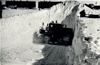
Fig. 4. Excavating a pit

Equipment

All physical measurements were made using USA SIPRE’s “standard” glaciological equipment. This consists mainly of: (1) a snow kit containing density tubes (6 cm. diameter, 500 cm.³ capacity) and spring balance, and bimetallic dial thermometers, (2) a 7.6 cm. diameter snow-ice coring auger with 1 m. extension rods,Reference Bader ²⁵ (3) a rammsonde cone penetrometer for hardness measurements, and (4) a portable resistance thermometer and copper thermohm cable,Reference Wade ²⁶ for deeper and more accurate temperature measurements. Various other supplementary pieces of equipment were also used.Footnote *

Method of Study

All precipitation on a high polar glacier falls as snow and each year the new snowfall buries the previous accumulation. By excavating a pit and systematically measuring the physical variations and stratigraphie differences exposed in the firn profile it is possible to identify the increments which correspond to the net annual accumulation. The entire concept of a pit study is based on the cyclic recurrence of certain seasonally related physical features, preserved in the firn profile. The most important are those caused by seasonal weather changes, such as ice layers, icy-firn, melt crusts, depth hoar and wind crusts; combined with density differences. The firn profiles in the different zones of the ice sheet each have their own distinguishing characteristics, but since they are weather dependent and because of the number of variable factors involved, the accumulation record often shows some irregularity. The final value of a pit study rests on the ability of the investigator properly to interpret the often less than systematic record of the firn profile and to reconstruct an accurate and reliable accumulation record.

Basically, pit studies may be divided into two major aspects: (1) the stratigraphie study, which includes all of the physical measurements and visual observations made on the firn layers; and (2) the temperature study, which reveals the thermal gradient, and, at the 10 m. level, a close approximation to the mean annual surface temperature. Descriptions of the different methods and techniques employed for accumulation measurements are scattered throughout the literature. The most complete and detailed modern discussions on the subject are by SchyttReference Schytt ¹⁶ and Benson.Reference Benson ¹⁷ The great advantage of pit studies over other methods of measuring accumulation, such as stakes or gauges, is the ability to obtain the preserved record of several years’ accumulation without returning to the area. A definite procedure has not yet been universally adopted, but most investigators collect compatible data.

Procedure and Techniques

When a pit location was reached the site selected for pit study was outlined with markers as guides for the tractor (Fig. 5, p.1034). The face wall was always aligned so as to be in shadow throughout most of the investigation, and particularly before the near-surface temperatures were measured. While the pit was being excavated, a 4 m. deep bore hole was augered nearby into which the thermohm cable was inserted to acquire temperature equilibrium with the firn at this depth. As soon as the pit had been excavated (about one hour), a section was trimmed back and dial thermometers were inserted at 10 cm. intervals over the exposed profile. Later, adjacent to the temperature readings, density measurements were made and the stratigraphy was studied in detail. The rammsonde measurements were usually conducted 1 to 2 m. away from the pit wall before excavation began. A bore hole was augered from the bottom of the pit floor to the 10 m. depth for the deeper temperature measurements. This drilling provided a 7.6 cm. diameter core for density measurements and observation of prominent structural features. A complete pit study usually required about 24 hours of continuous work by two men.

Fig. 5. Studying a pit wall

General Observations

For convenience Pit 0 (Fig. 6) will serve to illustrate and summarize the detailed observations and measurements made at each pit. This shallow pit is located 26 km. from the edge of the ice sheet and is approximately on the firn line (Schytt,Reference Schytt ²⁰ p. 47). The snow cover this early in the year (May) represents the net gain in deposition since the previous Summer’s ablation period. The strata are well defined and the distribution of the physical properties of the firn are nearly ideal over the vertical profile. The undulating snow-ice interface is a product of the 1958 surface melt and runoff. Below this are icy-firn (refrozen water saturated firn), ice layers and glacier ice. A characteristic of a new snow cover blanketing a previous melt surface, as seen in this figure, is the formation of a depth hoar layer above the interface. Moving up the profile from the coarser and loosely packed autumn snow, which was also affected by the sublimation process, there is a gradation into the denser wind-packed and finer-grained snow deposited during the severe winter months. Maximum density and hardness values are usually associated with the winter layers. The early spring deposit is softer and less dense, being younger and less affected by wind action. Note also that the stratigraphy is in close agreement with the physical measurements. The nearly isothermal condition between 20 and 70 cm. is due to the influence of the winter cold wave which, however, has been greatly modified by heat transfer from below. Evidence of this modification is still seen below 70 cm. The upper 20 cm. of the temperature curve reflects the beginning of the summer period.

Fig. 6. General Observations and measurements

This is the close agreement that normally can be expected between the physical measurements and stratigraphic features in pit studies. It is a systematic sequence such as this, repeated annually, that one attempts to distinguish in the deeper pits at higher elevations. One must bear in mind that the profiles change with time. In the above example, the accumulation is almost completely removed by ablation in the succeeding few months.

Accumulation

Before discussing any of the results, it should be understood that only the data collected from the Iimited district traversed by “Operation Lead Dog” are used for the correlation analyses. When they prove useful, mention is made of results from other studies in adjacent areas, but no comparative evaluation will be attempted in this paper.

Discussion of Accumulation Results

Previous predictions indicated that the net accumulation above lat. 78°–79° N. was less than 10 g./cm.², although no direct measurements had been made. This estimate was partly based on: (1) the 12–14. g./cm.² found by BullReference Bull ²³ during a rammsonde survey conducted along the lat. 78° N. line in 1954, (2) the negative budget, of −5 g./cm.² per year, found by FristrupReference Fristrup ²⁷ from two years of stake measurements between 1948–50 on the Chr. Erichsens Brae on the Heilprin Land ice cap in Peary Land, and (3) on precipitation measurements from two near sea-level weather stations, Nord and Alert.

About 75 rammsonde profiles were made on “Lead Dog” and Project 36. It was found from these studies that making stratigraphic inferences from rammsonde profiles for accumulation purposes was at best only fair, and then only when compared with observations and measurements made on the exposed walls of a pit. It was hardly possible to interpret annual or seasonal layers with any confidence with only the rammsonde profile. FristrupReference Fristrup ²⁸ in discussing the climatological conditions existing in Peary Land states that the Jørgen Brønlunds Fjord area of Peary Land has the highest continentality factor of all of Greenland and also that Station Nord is greatly influenced by open water. Furthermore, he contends, both locations have decidedly different meteorological conditions than the central portion of the inland ice sheet. Similar remarks apply to Station Alert. It is concluded, therefore, that conditions existing at coastal stations or small ice caps surrounded by a continental environment, and the climatic conditions at higher elevations on the inland ice sheet, constitute two different environments and should not be the bases of a climatological comparison.

The systematic variation and distribution of accumulation reported here is in good agreement with pit studies conducted further south by BensonReference Benson ¹⁷ and Koch and WegenerReference Koch ⁹ in that the greater accumulation is found on the western slope at lower elevations and the lesser inland at higher elevations. We can now add that similar conditions prevail on the northern slopes of the ice sheet, which are supplied with moisture from the Arctic Ocean Basin. Cyclonic storms which pass in an easterly direction over the northern sector of the ice sheetReference Matthcs ^{29 ,} Reference Matthes and Belmont ^{30 ,} Reference Hamilton ^{31 ,} Reference Hamilton ³² can with their counter-clockwise wind systems pick up moisture from warm pack ice, open water and leads (Fig. 11, p. 1035); and the air masses, emanating from the Arctic Ocean Basin, which are instrumental in creating the drift pattern of the pack ice and ice islandsReference Worthington ^{33 ,} Reference Browne, Crary and Bushnell ³⁴ also contribute. The north slopes serve as orographie barriers causing precipitation. Storms occurred at both the Nyeboes Land and Peary Land “Lead Dog” base camps.Footnote * Within three-day periods, at both camps, north winds deposited between 16 and 22 cm. of new snow (4 to 6 cm. of water equivalent). This was summer accumulation which would most likely waste away at these low elevations, but it does indicate the magnitude of accumulation that can fall on the northern slopes during a single storm.

Fig. 11. Open leads off Gape Bryant, Nyeboes Land, June 1959

This investigation was confined to the inland area above 1,400 m., which simplifies the analysis, since apparently a more uniform depositional environment exists in the interior, but, in addition, it is also the stable interior that provides the largest area for accumulation. This study reveals a general net accumulation rate for inland north Greenland of the order of 18.5 g./cm.² per year (mean of the means).

BauerReference Bauer ³⁵ gives 1.7264 × 10⁶ km.² as the total area of the Greenland Ice Sheet. The area above lat. 78° N. is approximately 0.34 × 10⁶ km.², or about one-fifth of the total. This is large enough to affect any total mass balance calculation for Greenland, if the accumulation estimate is off by a factor of two. From his studies of north and central Greenland, Benson,Reference Benson ¹⁷ has revised the mean net accumulation value for all of Greenland to 34 g./cm.² and claims that a slightly positive net balance exists. The “Lead Dog” results favor a positive budget for north Greenland, and when combined with Benson’s results accentuate the positive mass balance for the entire Greenland Ice Sheet. A recent report by BaderReference Bader ³⁶ (personal communication) which includes all available accumulation data up through 1960 gives 36.7 g./cm.² as the mean accumulation for the whole ice sheet.

Temperatures

Early studies by SorgeReference Sorge ³⁷ and others have indicated that the 10 m. temperature of firn in a dry-snow zone is close to the mean annual surface temperature. This was later confirmed for north Greenland by H. Bader and G. E. Frankenstein at Site 2 by averaging daily surface measurements carried on over two Summers and a winter season and comparing them with those obtained from a 30 m. deep pit dug at the same location.Reference Bader ¹⁹ A similar correlation was obtained for north Greenland at the B.N.G.E. station “Northice” (18 months meteorological dataReference Hamilton and Rollitt ^{38 ,} Reference Hamilton and Rollitt ³⁹ ) For this reason, the temperature measurement at 10 m. was considered of great importance and always obtained. Table VI summarizes the resistance thermometer measurements.

All snow temperature measurements are plotted in Figures 12a, 12b and 12c. They are separated into three groups for clarity. In the Summer, the temperature decreases with depth below the surface, and during the Winter the reverse situation will prevail. The large temperature gradient in the upper 2 m. of the first five pits illustrates the effects of the approaching Summer at these locations. Between 2 m. and 6 m. at these sites a remnant pulse of the Winter’s cold wave is still quite evident, but gradually diminishes to zero around 8 m. From 8 m. down, with the exception of Pit 1, all curves in Figure 12a show negligible slope changes. The effect of the rapidly developing Summer can easily he followed in the temperature profiles from the Nyeboes Land leg of the traverse (Fig. 12b). Curves 6 and 7 maintain a fairly constant temperature difference over their entire depth, but the 20 day time span between measuring Pits 7 and 8 has greatly altered the profile of Pit 8 in respect to the others. A recognizable relic of the Winter’s cold wave can still be seen in curves 6 and 7 but is hardly perceptible in 8. In the family of curves representing the final leg of the traverse to Peary Land (Fig. 12c) no evidence of the cold wave remains, even at the higher elevations of Pits 9 and 10. The split curve above 6 m. at Pit 11 is a result of an interruption in measuring the temperature profile because of a storm. The dashed line represents the actual values obtained from the dial thermometers in the pit wall after the storm passed; the solid line is the reconstructed curve based on the measurement made at the 4 m. hole a short distance from the pit waIl.

Fig. 12a. Temperature profiles from Pits 1–5

Fig. 12b. Temperature profiles from Pits 6–8

Fig. 12c. Temperature profiles from Pits 9–12

Discussion of Temperatures

In Figure 13, firn temperatures from the 10 m. depth are plotted as a function of altitude. The temperatures are accurate to ±0.1° C. and the elevations are reported accurate to ±10 m. There is some uncertainty on the usefulness of the values from Pits 1, 7 and 8, since these locations are subjected to a considerable amount of melting during most ablation periods which could have altered the relation to surface temperature (see Schytt,Reference Schytt ²⁰ p. 52). The mean temperature gradient for the entire traverse is 0.77° C. per 100 m. This value is close to the calculated mean lapse rate of 0.74° C. per 100 m., given by DiamondReference Diamond ² for all of Greenland. It is interesting to note that the sea-level intercept for this empirical line, –12° C., is close to the mean annual air temperature for the near-sea-level station at Thule, and when the proper temperature-latitude correction is applied (1° C. per 1° latitude), also for Station NordReference Fristrup ²⁸

Fig. 13. Temperature versus elevation curve

BensonReference Benson ¹⁷ expresses a view that the surface temperature gradient in an east-west direction at lat. 77° N. is controlled by the persistent katabatic winds that flow down-slope and are being heated adiabatically. This process appears to account for his temperature gradient of about 1° C. per 100 m. The temperature gradient between Pit 1 and Pit 9, in a direction north of east is in direct agreement with Benson’s. If the wind systems do have a major control over the temperature gradients, a possible explanation for the 0.63° C. per 100 m. gradient measured on the Nyeboes Land slope would be that it is controlled by the moisture saturated north winds, rising with the wet adiabatic lapse rate of 0.6° C. per 100 m.

A brief study of Figure 13 shows certain linear trends that appear to be associated with the different legs of the traverse and latitude. Tables VII and VIII present a summary of these different temperature-altitude gradients.

Figure 14 shows the surface distribution of the mean annual temperatures. The isotherms have been extended south to tie in with measurements made by other investigators. Stations measured in the heavy melt areas, in which the reliability is less, are connected with a dashed isotherm.

Fig. 14. Mean annual surface temperature contours for north Greenland

Figure 15 shows the interrelationship of latitude and temperature and Table IX summarizes these data. Only the central inland dry snow locations were used to avoid large altitude corrections and to avoid possible marine influence. The temperature values from each location were adjusted to 2,132 m., the mean pit elevation of the sites being considered, using the average gradient of 0.77° C. per 100 m. No correction was applied for the longitudinal dispersion of the sites. This figure shows a negative gradient of about –1° C. per degree latitude north.

Fig. 15. Temperature versus latitude curve

Pits 2 and 3 are also listed in the table since they are above 2,000 m., although strictly they lie outside of the dry snow zone.

The accumulation versus temperature relationship is shown in Figure 16. This empirical correlation curve indicates a smaller accumulation with a decreasing environmental temperature. The linear fit for most stations is rather good and implies that a proportional relationship exists between temperature and accumulation on the inland ice. Note also that there are no systematic deviations depending upon geographical location. From this relationship, it is also possible to delineate the dry snow, transitional and heavier melt regions for this district of the ice sheet. There is an interrelationship between accumulation, temperature and elevation that may be observed in the empirical regression equations contained in the Appendix C.

Fig. 16. Accumulation versus temperature curve

Density Variations

A fundamental characteristic of the firn at any location, and indicative of the environment, is its density. Any significant seasonal or climatic change that may have occurred in the past is registered in the density profile. This sensitive response of density to climatic variations is a great aid, and is often used to interpret seasonal and annual layers. By expanding this analysis, it may be possible to use the mean density of a pit profile as an environmental indicator, representing the summation of past climatic events.

Wind and temperature are discussed by SchyttReference Schytt ¹⁶ as being the two most important factors influencing the density of new snow, but in addition, further changes take place after deposition, and these changes tend to be characteristic for each location. Generally, firn density is increased by natural compaction or by melt action and refreezing, both dependent on local temperature conditions.

For the following analysis only the density values obtained from the exposed wall of the pit were used. The mean density over this profile,

(see Appendix C) was computed by integrating the individual densities over the depth interval of the pit. The ice layers and icy-firn contained in each annual increment were included, and for purposes of computation, taken as 0.9 g./cm.³ and 0.45 g./cm.³ respectively. To standardize the reference level, all calculations start with the 1958 accumulation year, and extend to the base of the pit. Since all pits except Pit 1 were excavated to about the same level, nearly equivalent depth profiles are being considered from each location. Small differences in depth have little significance to the mean density value, since the greatest density variations occur nearest the surface.

Figure 17 shows the mean density plotted against elevation, and a line is drawn. There is less scatter at the higher inland dry-snow locations and also at the lower elevations where melt is observed each year. In the transitional zone, where the melt is not as regular and varies in intensity from abundant melt during one Summer to sparse or no melt in others, the values can be expected to deviate. The least squares computation gives a mean density gradient of about 8 × 10⁻⁵ g./cm.³ per 100 m. Figure 18 compares the mean density with the mean annual temperature. This empirical correlation shows a density gradient of about 8 × 10⁻³ g./cm.³ per degree. In Figure 19 we see the mean density plotted against mean net accumulation. The empirical regression equations for the density data, contained in Appendix C, show interrelationships similar to the accumulation data.

Fig. 17. Mean density versus elevation curve

Fig. 18. Mean density versus mean annual surface temperature curve

Fig. 19. Mean density versus mean net accumulation curve

Conclusions

This snow investigation on the inland ice of north-west Greenland has brought out several interesting facts about the general climatic conditions existing in the region. Evaluation of the data summarized in this paper leads to the following general conclusions:

1. Elevation, direction and gradients of surface slopes, temperature, wind conditions and distance from the source of moisture are controlling factors in the accumulation rates.

2. The average temperature gradient is similar to the average for all of Greenland, but distinctly different gradients exist for the different traverse legs. Elevation is shown to be a major factor, however latitude, and also direction and gradient of surface slopes, are involved.

3. The mean density at a location is shown to be an environmental indicator.

4. A larger accumulation rate exists for north Greenland than was previously assumed.

5. The north slopes of Greenland are supplied with precipitation brought in by rising air masses which obtain moisture from the Arctic Ocean Basin.

Acknowledgements

The author wishes to express his appreciation for the support and cooperation received from the USA TREOG. The use of position and elevation values, obtained by the Navigation Section, is also gratefully acknowledged. Special thanks are extended to R. E. Hogan, who served as field assistant during the entire operation. H. Roethlisberger kindly processed the statistical data and H. Bader critically reviewed the manuscript.