1. Introduction

The size, velocity, and probably stability of glaciers are determined in large part by how the glacier interacts with its bed. The bed may be rugged so that ice must flow over and perhaps around the obstacles. There may be variations in the amount of subglacial drag or water such that in some places the glacier can slide easily and in others hardly at all. These processes are difficult to study at any scale because of the inaccessibility of the bed and because large-scale processes cannot be reproduced properly in the laboratory.

Here we develop a theory and a technique for investigating how glaciers negotiate variations in their beds. The theory relates stress applied at the bottom surface to the resulting effects, such as internal strains and surface topographic variations. The effects can be measured and data from near Byrd Station are used to indicate the sort of basal variation that most influences the ice flow.

The theory is an improvement on the work of Reference BuddBudd (1970) and has strong similarities to that of Reference HutterHutter and others (1981). Flow variations are superimposed on an average flow. One of the strengths of this approach is that it is not necessary to obtain a solution for the average flow if data or estimates of average flow velocities are available. Thus flow variations can be studied even if there is some uncertainty in the dynamics of the overall glacial flow.

Data used to test the theory and apply the technique come from the Byrd Station Strain Network (BSSN), in Antarctica. This array of movement poles is approximately aligned along an ice flowline from the ice flow divide to Byrd Station, 162 km distant. At Byrd Station a core hole penetrated to the bed of the glacier, where water was encountered (Reference GowGow, 1970). Characteristics of ice flow along the BSSN are reported by Reference WhillansWhillans (1976, Reference Whillans1977, Reference Whillans1979, Reference Whillans1981, Reference Whillans and Robin1983).

2. Theory

Strain-rates and stresses are separated into averaged and variational components and linear viscous rheology is used. This means that variational components can be studied largely independently from the averaged values. In addition the solution involves the equations for stress equilibrium and the equation of compatibility for strain-rates.

Inertial forces may be neglected in glacial flow and so stress equilibrium is described by:

in which σ_ij is the stress tensor, ρ is the density, and g_i is acceleration due to gravity. Subscripts after a comma denote differentiation and repeated subscripts signify summed tensor components.

A rectilinear coordinate system is defined that lies along the mean surface of the glacier (Fig. 1) and stresses are the sum of longitudinally averaged stresses

and local variations :

Fig. 1. Longitudinal section to illustrate coordinate system.

For use later the averaging length L must be sufficiently long that gradients of averaged values of σ_xx and σ_zx are equal to gradients calculated using spot values separated by the distance L, that is:

If L is sufficiently long and the “noise” due to local variations sufficiently small, Equation (3) is valid. For the BSSN a value of L on the order of 100 km would be appropriate, although it is not necessary to specify L only to note that Equation (3) could be satisfied by some L.

This discussion of averaging lengths would not be needed if the σ ^v could be considered as perturbations to the σ ^a. In practice however the variation of stresses are of the same order of magnitude as the averaged values and they can not be studied as small-order perturbations.

Equation (1) is now averaged:

or

or

and using Equation (3):

Thus gravitational body forces are associated with the average stresses. Unlike Reference HutterHutter and others (1981) we have included all average stress components in this equation.

Combining these Equations (4) with Equations (1) and (2) provides:

Gravitational forces do not enter the solution for stress variation except at the boundaries (included later). Equations (5) are the first set of equations that are used in the present model.

The flow of the glacier is taken to be two-dimensional. This is a fair approximation for the flow near Byrd Station, Antarctica, where there is a small but uniform divergence of flowlines. Transverse strain-rates (Fig. 2b) are smaller and change less than longitudinal strain-rates (Fig. 2c) and the flowline is nearly parallel with the strain network (Fig. 2a). We suppose that variations in strain-rate and stress deviators that involve transverse components may be neglected.

Fig. 2. Measured quantities from the Byrd Station Strain Network. Byrd Station is at 162 km, and the ice divide at 0 km.

For two-dimensional deformation, the equation of compatibility for strain-rates

is:

and, as with the stresses, the strain-rates are separated into averaged values and variations:

and so

The strain-rates

describe longitudinally averaged flow and so, necessarily, longitudinal gradients in are very small and the terms and are set to zero. The assumption is now made that the averaged, longitudinal strain-rate is constant or a linear function of depth so that is zero. Later is calculated and found to approach zero for long wavelength features, so the model is internally consistent. Setting these terms to zero, Equation (7) reduces to:

which is the form used in the present model.

Strain-rates are taken to be isotropically related to stress according to:

in which η is effective viscosity. The prime (′) indicates deviatoric stress. For two-dimensional flow the full transverse stress is equal to

and deviatoric stresses are:

and

Reference BuddBudd (1970), in effect, assumed that

and hence that the spherical stress does not vary, but that assumption is not in line with usual concepts of ice deformation.

Separating the stresses and strain-rates into averaged and variational values (Equations (2) and (6)) and substituting:

or

It is now necessary to define separate viscosities, η ^a and η ^v, so that

Equation (9) is used in this analysis.

If ice were Newtonian viscous, η ^a = η = η ^v, and the maneuver leading to Equation (9) would be strictly correct. Ice however is usually considered to have a stress-dependent viscosity, and in the present theory some of this dependency can be viewed as being included in η ^a. Stress and strain-rate variations from the average flow are however modelled as being linearly related. This is not a severe limitation for small variations but the results for large stress variations must be viewed as being only approximately correct.

A depth variation in effective viscosity can be included:

for η ₀ and r constant. This depth variation would be related to variations with depth of octahedral stress, temperature, and perhaps the effects of changing ice structure. This feature is included in the mathematical solution but for simplicity a constant viscosity η ^v is used in the application of the theory to ice flow along the BSSN.

The model is formulated in Equations (5), (9), (10), and (8). The next section develops the mathematical solution to these equations.

3. Mathematical solution

It is convenient to define a function ϕ such that:

and this ensures that Equation (5) is satisfied.

The strain-rates are, by Equations (9) and (10):

and substituting this into the equation of compatibility (8):

or

Seeking a function that is periodic in x, try

in which

and real roots are to be used. We note that solutions for different ω can be added. Equation (11) becomes:

The superscript numbers in parentheses denote the level of differentiation.

Next try an exponential depth variation in f:

and so

or

which is quadratic in β(β + 1), the roots of which are:

This is quadratic in β and

These four independent solutions fully satisfy Equation (12).

Substituting back, the solution to Equation (11) is obtained:

in which

or writing just the real part of ϕ:

For the case of constant viscosity, r = 0, the solution is more simple:

In the following analysis this latter, simple form for the case of constant viscosity is used. The fuller equation could be carried through but we have not done this.

The constants a_i are obtained from appropriate boundary conditions, and to help in that topic the following is a list of useful quantities:

The horizontal velocity variation is

The vertical velocity variation is

and the spherical stress (sometimes called hydrostatic stress) variation is

4. Boundary conditions

The physical model envisioned has prescribed variations in bottom topography and in basal sliding. Other quantities including the surface topography are determined by these basal variations and by ice-flow characteristics. Mathematically however, basal characteristics are linearly related to surface effects and it is mathematically equivalent to prescribe surface and bottom topographies (or surface topography and bottom sliding) and calculate other basal variations. This method also leads to simpler equations and it is used here.

Four boundary conditions are needed because there are eight unknowns, the a_i , and each boundary condition results in two equations, one including sin ωx and the other cos ωx. Two of the boundary conditions require the ice-flow variations to follow the top and bottom topographies and two further conditions relate to stress variations at the top surface (z = 0).

Reference BuddBudd (1970) used the two boundary conditions requiring the ice flow to follow the upper and lower surfaces and harmonic loading of the surface as used here. He supposed that the spherical stress variation,

, is everywhere zero so that a ₂, a ₄, a ₆, and a ₈ are zero. The physical model behind this last constraint is not clear, and it is mainly because of this that the results of the present theory are different from Budd’s.

In this work the boundary conditions are used to express the a_i in terms of the surface and bottom topographic reliefs, for which there are data along the BSSN. Then, in the next sections, a number of other quantities are calculated. First, the surface strain-rate variation is derived and compared with data, and this leads to a value for the effective viscosity of the ice. Then in section 6 the basal variations that cause the observed ice-flow variations are calculated and discussed.

One of the merits of this approach is that it is not necessary to first discuss the physics of basal action: rather data are used to indicate the nature of basal variations, from which we later infer some features of the dominant physical processes.

The coordinate system is defined with z = 0 at the mean top surface and z = H at the mean bottom. In general there are variations in both surfaces. Let the top surface elevation vary according to:

and the bottom surface elevation according to

The values of B_s and B_c determine the magnitude and phase of the bottom surface with respect to the top surface.

5. The viscosity

The solution can be tested against data from the Byrd Station Strain Network (Fig. 2). First, however, it is necessary to select appropriate values for the frequency ω of stress and strain-rate variation, for the amplitude h ₀ of surface topographic variation, and for effective viscosity η ^v.

Common variations in strain-rate, surface topography, and internal layers occur at scales of 10 to 40 km (Fig. 2c, d) but for convenience we discuss mainly variations of 10 km (ω = 2π/10 km) and discuss briefly how results for variations on the 40 km scale differ.

From Figure (2d) the amplitude of topographic variation is about 2 m.

The longitudinal strain-rate variations at the top surface are described by:

From Figure 2g the surface velocity is about

. Basal velocities are slower and seems reasonable. Substituting in addition h =3 000 m, h ₀ = −2 m, for a 10 km wavelength variation:

for B _s and B _c in meters. The basal relief (Fig. 2e) is less than 40 m and the observed amplitude of longitudinal strain-rate variation (Fig. 2c) is about 5 × 10⁻⁵ a⁻¹, so the first term must dominate and the appropriate value for the viscosity, η ^v, is about 10⁸ N m⁻² a or 1 000 bar a. This value is about that expected from flow laws commonly used to describe glacial flow at temperatures of −30 °C, and stress 0.1 to 1 bar, as are applicable here.

Neglecting the smaller terms, the strain-rate variation at the top surface is. to a first approximation:

The factor ρgh ₀/2η ^v describes the sinking of the surface undulation into the rest of the glacier due to its own weight. For features long compared to the ice thickness the bottom inteferes with this process according to the second term. For wavelengths of 10 km (3H) that term is about 0.5 and is 0.9 for wavelengths of 40 km, and we note that for surface undulations of equal amplitude, the shorter wavelength features are associated with larger strain-rate variations. This is important in mass-balance studies where regionally representative strain-rates need to be measured.

This last equation also demonstrates that, at least near Byrd Station, the phase or even the amplitude of bottom topographic variation is not important to the relative magnitudes of h ₀ and surface strain-rate variation. Of course both the surface strain-rates and the surface topography are caused by basal variations, but it woud be difficult to obtain information on basal mechanics from the relative amplitudes and phases of surface topographic and surface strain-rate variations.

The procedure of comparing h ₀ to

has led to a value for the effective viscosity, which has been taken to be constant with depth. In reality the effective viscosity is expected to decrease with depth due to the effects of increasing temperature, octahedral stress, and other factors. Such a depth variation in effective viscosity has been treated by Reference RasmussenRasmussen (unpublished) and Reference JohnsenJohnsen and others (1979) by using a three-layer model, each layer of which is treated in a manner similar to that in the present work, but with each layer having a different viscosity. Reference HutterHutter and others (1981) also show how these effects can be included in a numerical solution. Our viscosity is derived largely from surface data so the calculated value applies mainly to the cold, viscous upper portion. A value less than 1 000 bar a could be used but we choose to retain this value because it leads to conservative results later.

In the development of the theory it was assumed that the longitudinal strain-rate

was constant or varied linearly with depth. The predictions of the theory do not contradict this. Calculated longitudinal strain-rate variations on a 100 km scale are very small (two orders of magnitude less than those associated with variations on a 10 km scale). This is not a test of the validity of the theory, but at least the model is internally consistent.

6. Derived quantities

Our approach is to calculate basal properties using surface data and radar sounding results. In this section we derive the variations in basal shear stress, basal sliding, and basal pressure.

The basal shear stress is

and, substituting values as before,

for B _c and B _s in meters. The basal amplitude is usually 40 m or less along the BSSN and the terms involving that can be as large as 0.10 × 10⁵ N m⁻². Thus the amplitude of basal shear stress variation is 0.3 to 0.4 bar and is about 90° out of phase with the surface topography. The first and dominant term is independent of the value for effective viscosity and the bottom topography influences the basal shear stress only secondarily.

These conclusions also apply for features of wavelength 40 km except that surface features of amplitude 2 m can be generated by basal drag variations of amplitude only 0.08 bar.

The mean shear stress along the Byrd Station Strain Network, at z = H, is about 0.4 bar, so local basal shear stresses vary between near zero and about 0.8 bar.

Basal pressure variations are described by:

for B _s and B _c in meters. Once again the first term dominates and its value is independent of η ^v.

Basal sliding variations are:

for B _s and B _c in meters. For B _s or B _c equal to 40 m the second terms in each parenthesis are ±0.07 m a⁻¹. The dominant term is very sensitive to the value of effective viscosity η ^v, and our value of 1 000 bar a may be too large, in which these calculated basal sliding variations are too small.

Thus near Byrd Station, at least, ice-flow variations are caused mainly by variations in bottom sliding (basal drag and perhaps pressure) and only to a lesser extent by flow into and out of the basal topography.

To simplify the discussion, examples are shown in Figure 3 of the quantities calculated above. In each case basal conditions have been selected so that the surface topographic relief and surface strain-rate variations match the data. In the example at one extreme. Figure 3a, the bottom is taken to be flat but there can be sliding variations. At the other extreme. Figure 3c, the basal topography has been selected so that there is no variation in bottom sliding (Equation (21)). This topographic amplitude is about 100 m: much larger than is common along the BSSN, although there are examples. If a lower-valued viscosity were used an even larger basal topography would be needed. The intermediate model. Figure 3b, uses B _s = −40, B _c = 0 as is often observed. The examples of Figure 3a and b seem to best describe conditions along most of the BSSN.

Fig. 3. Ice flow characteristics for three models of basal variation (a) flat bed with sliding variation, (b) intermediate, and (c) undulating bed with no sliding variation.

A possible shortcoming of the theory may be supposed from Figure 3a and b. Basal velocity variations are about 2 m a⁻¹ which is comparable to expected values of

. This violates a simplification made in deriving the second boundary condition. However, in the model of Figure 3a, , and so w ^v = 0, and the boundary conditions expressed by Equations (15) and (16) can be obtained without making an assumption about the magnitude of basal sliding variation. This problem applies to the model of Figure 3b, but that calculation could more correctly be done by adding solutions like those of Figures 3a and c.

Vertical and horizontal velocity variations for two of the models in Figure 3 are displayed in Figures 4 and 5. Vectors directed to the left indicate slower than average flow. As would seem reasonable, slower basal sliding is found to be associated with larger basal shear stresses. Where basal sliding is slow (and basal drag large) and the ice ‘rides up over’ the difficult flow section (note the faster velocities in the upper part of the ice sheet) and conversely, over regions of faster basal slip, the ice is drawn down and there is faster flow in the lower portion of the glacier.

Fig. 4. Flow variations for a flat bed with sliding variations. The vectors are to be added to the average flow. Slow, fast and slow sliding regions alternate. The model corresponds to Figure 3a.

Fig. 5. Flow variations for an undulating bed and sliding variations, and corresponding to Figure 3b.

These velocity variations may be integrated to show how lines in the glacier are distorted (Fig. 3). The vertical displacement of a particle is:

in which t represents time. The integration is changed to horizontal distance by using

and noting that except perhaps near the base of the glacier u ^v ≪ u ^a:

The wavy lines at several depths in Figure 3 demonstrate how an isochrone or a particle path is distorted by flow over a varying bottom. Internal radar-reflecting layers near Byrd Station are believed to be associated with isochrones (Reference WhillansWhillans, 1976) and so these lines should also model distortions in radar layering.

7. Distortions of radar-reflecting layers

The observed distortion of radar layering (Figs 2f and 6) is in close agreement with theory (Fig. 3). The phase relation between layer distortion and surface topographic and strain rate variations is exactly that predicted, thus providing a strong positive test of the theory. The amplitudes of the 10 km scale distortions are mainly within a factor of two of the amplitudes predicted by the models of Figure 3a and b. Some of the distortions are larger than predicted and some smaller. The distortions are often associated with bed topographic variations but sometimes there is no corresponding topographic feature (for example, at 130 to 140 km in Figure 6). Other radio echo-sounding flights across and parallel to the Byrd Station Strain Network indicate that transverse topographic variations cannot explain this anomaly.

Fig. 6. Top and bottom surfaces and selected internal radio-reflecting layers along the BSSN.

The best example from near Byrd Station of layer distortion not associated with bed topography is shown in Figure 7. This is from a site just to the right of the Byrd Station Strain Network (looking with the ice flow) at about x = 150 km, and labelled “fold” in Figure 2a. The interpretation of the photograph is complicated by a multiple reflexion from the aircraft and the position of the bottom may not be best reproduced in publication. Therefore, Figure 7 also shows a tracing of the relevant features. The layers are distorted downward near sites of bright basal reflexion. The bright returns may be associated with subglacially ponded water, lower basal drag, and faster sliding. Certainly the layer distortions are consistent with a model (Fig. 3) of ice flowing alternately over lakes and rougher, high-drag regions.

Fig. 7. Radar record (a) and a tracing (b) of relevant features from the site labelled “fold” in Figure 2a. These data and those of Figure 6 were obtained by D. J. Drewry under the NSF–SPRI–TUD radio echo-sounding program.

Evidence for subglacially ponded water in the BSSN area was reported earlier (Reference WhillansWhillans, 1979). In that work a model for the general flow of the glacier was used that assumed a regular increase in basal sliding along the flowline. The model failed to match the data in the region near 150 km and subglacial lakes and hence faster sliding in that area were suspected. That concept is consistent with the predictions of Figure 3a, internal layers are drawn down over and a little up-glacier from regions of low drag and faster sliding.

Usually internal layer distortions are in phase with the bottom topography (Fig. 6) this is the reason for selecting a bottom topographic variation of the phase shown in Figure 2b. The flow variations are however due to variations in basal sliding and drag as well. Observation thus indicates that topographic highs are also sites of slower sliding and increased drag.

Although this result seems intuitively correct the reasons for this relation are not known with certainty. We speculate that topographic highs are swept clear of soft, slippery sediment and that water or malleable sediment such as till collects in topographic lows.

Subglacial pressure variations have a small effect on subglacial water flow. Figure 2b shows that the range of pressure variation is about 0.5 bar for the favored model. Water flows in response to this pressure variation together with gravitational potential gradients. Combining these effects (bottom curves on Figure 3) we find that water collects in topographic lows but with a slight bias toward the lee of topographic highs. This is similar to the effect discussed in sliding models but these models are concerned mainly with bed variations of shorter wavelengths. The tendency for water to collect behind topographic highs is weak and most probably other controls, such as those associated with channel development or bed permeability, are also important.

Interestingly, for the flat-bed model (Fig. 3a) water is driven from regions of low shear stress. If indeed the areas of low shear stress are lakes then the model of Figure 3a should be adjusted. The surface of the lake must be tilted downward in the direction of ice flow in order to counteract this effect. Perhaps this tilting could be detected by radar sounding.

Reference OswaldOswald (1975) studied tilted lake surfaces, but most of these lakes were near ice divides where there is little flow and the present effect would not be detectable.

8. Frequency dependence

Reference BuddBudd (1970) and Reference Budd and CarterBudd and Carter (1971) have used field evidence to demonstrate a dominance in the occurrence of surface topographic features with a wavelength of about three ice thicknesses. Along the BSSN features (Fig. 2d) of wavelength ranging from 7 to 50 km (two to twenty ice thicknesses) are present with 10 km (three ice thicknesses) being common. Very probably Budd and Carter’s finding applies here, but the BSSN is too short to properly test this.

The earlier version of the present theory (Reference BuddBudd, 1970) indicates a maximum in surface relief at a wavelength of three ice thicknesses (for ‘white’ basal relief) which suggests that the observed dominance is related to an internal ice-flow characteristic.

Different results are obtained here and by Reference HutterHutter and others (1981). Figure 8 shows the frequency dependence of transfer functions relating basal features to surface topographic variation. The two extreme models from Figure 3c and a are represented, these models are believed to bracket the behavior of real glaciers. Neither model shows an absolute maximum at three ice thicknesses although there is a minor peak in spectral power for a wavelength of three ice thicknesses in the constant sliding model (Fig. 8).

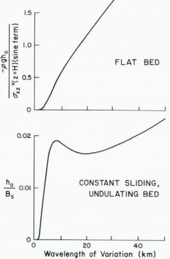
Fig. 8. Transfer functions relating the size of surface undulations to basal conditions as a function of wavelength.

The transfer function is the ratio of surface −h ₀ to bed amplitude B _s for the constant sliding model, and is the ratio of surface loading −ρgh ₀, which is linearly related to surface relief, to the principal component (the sine term) of basal shear-stress variation,

, for the flat-bed model. In this last model, the variation in basal sliding could be used instead of basal shear stress, and very similar results would be obtained.

The transfer functions demonstrate that the more extensive the basal variation, the more the flow is affected. In the case of the constant sliding model, a spectral maximum could be generated if the effective viscosity were less at longer wavelengths. The full ice thickness is however involved in all flow variations of wavelength greater than about one ice thickness (3 km) and a frequency variation of effective viscosity is difficult to imagine. Other processes must be responsible for the dominance of surface features of a wavelength of three ice thicknesses.

The results of Figure 8 can only be applied directly if the frequency distribution of basal variation is white, that is, if long-wavelength basal variations occur with the same amplitude as short-wavelength variations. The evidence indicates that basal variations are biased toward the shorter wavelengths of about 10 km and long-period variations in basal water thickness, or whatever is primarily responsible for flow variation, must be unusual.

Observation of formerly glaciated regions suggests that there are few roughness elements of horizontal dimension longer than 1 to 5 km, corresponding to a wavelength of between two and three ice thicknesses (for a former ice sheet 1 to 3 km thick). In eastern Canada, the most noticeable large features are accentuated by lakes which have this spacing. Why this should be so is not clear, perhaps it is connected with the processes of till deposition and basal erosion, or with subglacial water flow, or perhaps this spacing is inherited from an earlier episode of geologic activity, be it constructional as ocean-floor spreading in the case of Marie Byrd Land, or erosional such as river and slope activity during the Tertiary Era in Canada.

It has been suggested that intense horizontal shear zones within the glacier (Reference Gow and WilliamsonGow and Williamson, 1976), in effect, create a false bottom below which the ice is less active. The effective bottom would then be more simple than radio echo-sounding indicates and such a phenomenon occurs near the edge of the Greenland ice sheet (Reference ColbeckColbeck and others, 1978). We see no evidence for this along the Byrd Station Strain Network. For example, there is a major deep between 40 and 70 km (Fig. 6) yet the internal layers above this seem to be as much distorted as elsewhere.

9. Conclusions

The theory is able to explain many of the observed features of glacial flow and the method could be extended to other areas, including areas with less data. If a value for the viscosity can be assumed, perhaps the 1 000 bar a obtained here, it would not be necessary to measure detailed strain-rates. Surface elevation data together with the results of a radar sounding program could describe many features of the ice flow such as the existence or importance of subglacial sliding variations.

The models considered for the BSSN all allow for basal sliding, which seems reasonable because of the presence of subglacial water. A glacier that is not sliding could be modelled by an alteration of the model of Figure 3c. So that the bottom boundary condition (ice flow following the bed) has meaning, the “sliding rate”,

, would be the average velocity above an intense shear zone, and the ice “thickness” would be the depth to that zone.

In our opinion the main limitation to the theory is the use of a constant and isotropic viscosity, which is necessary for an analytic solution. We have, however, been conservative in our interpretation. The viscosity is derived from the relationship between surface topography and surface strain-rates, which is too large for describing effects near the bottom. A lower-valued viscosity would suggest an even greater importance of basal sliding variation.

The discovery of the great importance of basal sliding variation bears on discussions on the controls on glacial flow. The cause of these sliding variations is not known with certainty but their association with strong basal radio reflexions (Fig. 7) points to the role of ponded water. These water pools are almost certainly connected by channels or porous aquifers that drain down the hydrologic potential gradient. Other glacial changes may lead to a decrease in ice surface slope which in turn would reduce hydrologic potential gradients and increased ponding and faster flow. This is a positive-feedback mechanism and such developments have been suggested as the cause of very fast glacial flow as observed in ice streams and in surging glaciers.

In this regard it may be noted that there is a flow regime change about 160 km down-glacier from the end of the BSSN (to the right in Figures 2 and 6). Beyond that point the ice flows mainly in ice streams which have low slopes and fast speeds (Reference RoseRose, 1979).

Acknowledgements

We thank John Bolzan, Kenneth Jezek, and Niels Reeh for many helpful discussions. Much of the work was done when the authors worked at the Geophysical Isotope Laboratory, Copenhagen, Denmark. NSF grant DPP-7682032, supported the studies and R. Tope drafted the figures.

Note added in proof. An almost identical theory has been developed by Professor Louis Lliboutry who presented it in the course of a summer school (unpublished text of lectures, “Six leçons sur la dynamique des glaciers et calottes polaires”, given at the École d’Été d’Oceanologie Spatiale, Grasse, 1–28 July 1982, p. 55–58).