


Impact Statement
This study provides the first comprehensive characterisation of the instantaneous vortex flow around spinnaker sails. Spinnakers are used for running downwind, and thus operate at a comparatively low lift to drag ratio (i.e. low efficiency) compared with those sails used for sailing upwind, such as jibs and genoas. The study reveals that, despite the massive flow separation, twist does not change the lift curve slope. Hence, the same sail geometry could be optimal for different profiles of the atmospheric boundary layer, and the need for testing in facilities with a twisted onset flow can be relaxed. Furthermore, time-averaged flow reattachment does not necessarily result in a performance enhancement, as often anecdotally assumed for wings with significant flow separation, hence it should not be used as a design objective. Overall this paper paves the way to a conceptual design process for wings with massively separated three-dimensional flow that considers the force contribution of local flow features.
1. Introduction
Yacht sails are thin flexible wings. While modern sails have sufficient tension to behave mostly as rigid wings (Reference Gerhardt, Flay and RichardsGerhardt, Flay, & Richards, 2011), the term sail aerodynamics has traditionally been used to indicate the aerodynamics of flexible foils anchored at the edges. This canonical problem was pioneered by Reference CisottiCisotti (1932) and then followed by Reference VoelzVoelz (1950), Reference ThwaitesThwaites (1961), Reference Myall and BergerMyall and Berger (1969), Reference DuganDugan (1970), Reference Smith and ShyySmith and Shyy (1995) and Reference Lorillu, Weber and HureauLorillu, Weber, and Hureau (2002), etc. In contrast, the focus of this paper is on the aerodynamics of modern sails, which behave mostly as rigid thin wings. The field is described in the reviews of Reference MilgramMilgram (1972, Reference Milgram1998) and Reference LarssonLarsson (1990) and most recently by Reference ViolaViola (2013), as well as in the comprehensive books by Reference Whidden and LevittWhidden and Levitt (1990), Reference Claughton, Shenoi and WellicomeClaughton, Shenoi, and Wellicome (1998), Reference Larsson and EliassonLarsson and Eliasson (2000), Reference FossatiFossati (2009), Reference SlooffSlooff (2015) and Reference van Oossanenvan Oossanen (2018).
The most common rig, known as a Bermuda or Marconi rig, is made of one mast and two triangular sails: a foresail and a mainsail. The leading edge of the mainsail is attached to the mast and the aerodynamics of this configuration was investigated in detail by Reference WilkinsonWilkinson (1989, Reference Wilkinson1990). The foresail, instead, is attached to the boat only by the three corners. The flow field around foresails, which are wings with a negligible thickness and a sharp leading edge, is not well understood and it is investigated in this paper.
Specifically, the paper focuses on modern asymmetric spinnakers, which are used to sail downwind at true wind angles ( $\beta _t$) approximately over the range $100^\circ \leq \beta _t \leq 150^\circ$. Here, $\beta _t$ is the supplementary angle between the wind velocity and the course sailed by the boat. Asymmetric spinnakers are between the largest and most powerful sails carried by a yacht. As $\beta _t$ decreases below $100^\circ$, sails become smaller and flatter. These upwind sails are known as jibs and genoas, the latter being the largest of the two. In contrast, symmetrical spinnakers can be used over the same range of $\beta _t$ as asymmetrical spinnakers. However, they tend to perform better at the upper end of this range and can also be used at $\beta _t > 150^\circ$.
Symmetric and asymmetric spinnakers are often trimmed by letting the leading-edge fold periodically (Reference Aubin, Augier, Deparday, Sacher and BotAubin, Augier, Deparday, Sacher, & Bot, 2018; Reference Viola and FlayViola & Flay, 2010, Reference Viola and Flay2011a). This unsteady trim maximises the driving force at high  $\beta _t$, e.g. $150^\circ$ (Reference Viola and FlayViola & Flay, 2009). Conversely, at lower $\beta _t$, sails can be trimmed at higher angles of attack, preventing the leading edge from collapsing without a reduction in driving force (Reference Viola and FlayViola & Flay, 2009). In this scenario, the difference between a steady trim, where the leading edge is at the verge of collapse, and an unsteady trim with periodic leading-edge flapping vanishes. This applies to the flow conditions considered in this work. Furthermore, the membrane tension is high compared with the turbulence-induced load fluctuations, and thus fluid–structure interaction does not occur. For this reason, steady computational fluid dynamic simulations, where sails are modelled as rigid bodies, have been proven accurate in predicting the forces generated by asymmetric spinnakers, both at model scale (Reference ViolaViola, 2009; Reference Viola, Bartesaghi, Van-Renterghem and PonziniViola, Bartesaghi, Van-Renterghem, & Ponzini, 2014) and full scale (Reference Viola and FlayViola & Flay, 2011b). Hence, in this paper we use rigid models of asymmetric spinnakers.
Asymmetric spinnakers are thought to generate thrust through lift rather than drag, and thus designers tend to minimise flow separation (Reference Viola, Arredondo-Galeana and PisettaViola, Arredondo-Galeana, & Pisetta, 2021; Reference Richards, Johnson and StantonRichards, Johnson, & Stanton, 2001; Reference Whidden and LevittWhidden & Levitt, 1990). However, because of the sharp leading edge, this is not entirely possible. There is only one angle of incidence, namely the ideal angle of attack, where the onset flow is tangent to the leading edge and an attached boundary layer develops on both sides of the sail. At any other higher incidence, leading-edge separation occurs. The vorticity of the separated shear layer rolls up into free vortices, as in the wake of a plate at incidence (Reference Afgan, Benhamadouche, Han, Sagaut and LaurenceAfgan, Benhamadouche, Han, Sagaut, & Laurence, 2013; Reference Kiya and ArieKiya & Arie, 1977; Reference RoshkoRoshko, 1954, Reference Roshko1955; Reference SarpkayaSarpkaya, 1975). In some conditions, the advection of these vortices near the sail surface results, in a time-averaged sense, in flow reattachment and in a closed recirculation region near the leading edge known as a leading-edge separation bubble (LESB) (Reference Smith, Pisetta and ViolaSmith, Pisetta, & Viola, 2021). This is a feature akin to those experienced by thin aerofoils (Reference Arena and MuellerArena & Mueller, 1977; Reference Carter and VatsaCarter & Vatsa, 1982; Reference ChangChang, 1970; Reference Owen and KlanferOwen & Klanfer, 1953), flat plates at small incidence (Reference Crompton and BarrettCrompton & Barrett, 2000; Reference GaultGault, 1957; Reference Newman and TseNewman & Tse, 1992; Reference Stevenson, Walsh and NolanStevenson, Walsh, & Nolan, 2016) and circular arcs at low incidence above the ideal angle of attack (Reference CyrCyr, 1992; Reference Souppez, Arredondo-Galeana and ViolaSouppez, Arredondo-Galeana, & Viola, 2019).
On the aerodynamics of asymmetric spinnakers, several research questions remain unanswered. Because of the massive separated flow and high degree of twist, lifting line theory (Reference PrandtlPrandtl, 1918) cannot be used to predict the aerodynamic forces. Using lifting line theory, Reference PhillipsPhillips (2004) showed that twist increases the zero lift angle of attack of any wing, but that it does not affect its lift slope. Whether this conclusion holds for asymmetric spinnakers remains unknown.
Traditionally, studies on the aerodynamics of sails have focused on the time-averaged flow field (Reference Hedges, Richards and MallinsonHedges, Richards, & Mallinson, 1996; Reference Lasher and RichardsLasher & Richards, 2007; Reference Lasher and SonnenmeierLasher & Sonnenmeier, 2008; Reference Lasher, Sonnenmeier, Forsman and TomchoLasher, Sonnenmeier, Forsman, & Tomcho, 2005; Reference MilgramMilgram, 1998; Reference Nava, Cater and NorrisNava, Cater, & Norris, 2018; Reference Richards, Johnson and StantonRichards et al., 2001; Reference ViolaViola, 2009) and have emphasised the presence of the LESB and of the attached boundary layer that develops downstream of it. In contrast, only few and recent works consider the instantaneous vorticity field. These studies (Reference Arredondo-Galeana and ViolaArredondo-Galeana & Viola, 2018; Reference Aubin, Augier, Deparday, Sacher and BotAubin et al., 2018; Reference Deparday, Augier and BotDeparday, Augier, & Bot, 2018; Reference Viola, Bartesaghi, Van-Renterghem and PonziniViola et al., 2014; Reference Young, Morris, Schutt and WilliamsonYoung, Morris, Schutt, & Williamson, 2019) show that the flow on the suction side of the sail is only intermittently attached. It remains to be determined whether the high sweepback of the leading edge could result in a leading-edge vortex (LEV) that remains steadily attached to the sail, as opposed to vortices shed downstream and that result, in the time-averaged sense, in an LESB.
Reference Viola, Bartesaghi, Van-Renterghem and PonziniViola et al. (2014) and Reference Arredondo-Galeana and ViolaArredondo-Galeana and Viola (2018) hypothesised that, near the head of the sail, because of the higher sweep of the leading edge, the circulation shed by the shear layer might roll up into a three-dimensional LEV, where vorticity is convected through axial flow towards the tip. It has been shown, for example on plates at incidence, that low aspect ratios and high sweep angles such as those of spinnakers promote the advection of vorticity from the leading edge towards the tips (see the rich literature surveys on the effect of the aspect ratio in Reference Taira and ColoniusTaira and Colonius (2009), Reference Lee, Hsieh, Chang and ChuLee, Hsieh, Chang, and Chu (2012) and Reference DeVoria and MohseniDeVoria and Mohseni (2017), and on the effect of the sweep angle in Reference Huang, Venning, Thompson and SheridanHuang, Venning, Thompson, and Sheridan (2015)). Reference Viola, Bartesaghi, Van-Renterghem and PonziniViola et al. (2014), Reference Arredondo-Galeana and ViolaArredondo-Galeana and Viola (2018) and Reference Deparday, Augier and BotDeparday et al. (2018) found conflicting results on whether a stable LEV can remain attached to the leading edge of spinnakers. This could be enabled, for example, by vorticity extraction through axial flow that balances the vorticity production at the leading edge (Reference Akkala and BuchholzAkkala & Buchholz, 2017; Reference Eldredge and JonesEldredge & Jones, 2019; Reference Marzanek and RivalMarzanek & Rival, 2019; Reference Widmann and TropeaWidmann & Tropea, 2015). A stable vortex is found, for example, on delta wings (Reference Chang and LeiChang & Lei, 1996; Reference MaxworthyMaxworthy, 2007), on the wing's outer region (hand wing) of some gliding birds such as the swift (Reference Muir, Arredondo-Galeana and ViolaMuir, Arredondo-Galeana, & Viola, 2017; Reference Videler, Stamhuis and PovelVideler, Stamhuis, & Povel, 2004) and on autorotating seeds such as those of maples (Reference Lentink, Dickson, van Leeuwen and DickinsonLentink, Dickson, van Leeuwen, & Dickinson, 2009). However, whether a stable LEV occurs on yacht sails is still an open question.
The objectives of this paper are: (i) to investigate the effect of twist in the aerodynamic forces of asymmetric spinnakers, (ii) to assess whether time-averaged flow reattachment results in an enhancement of the sail performance (i.e. increase in driving force for a given side force value) as often assumed by sail designers (Reference Whidden and LevittWhidden & Levitt, 1990), (iii) to investigate whether there is a flow condition at which a stable LEV occurs and (iv) to provide the first comprehensive characterisation of the instantaneous vortex flow around a yacht sail.
To investigate these objectives, we built three different model-scale spinnakers, based on the same geometry but with different twist values, and tested the geometries in a water tunnel for a range of sail trims. The reference sail was designed for the AC33 class yachts. This class, which is a set of rules for the design of the boat and the sails, was proposed for the 33rd America's Cup – the world's oldest trophy in sport. While the AC33 class was never adopted because of a legal dispute between the Defender (Alinghi) and the Challenger (Oracle BMW), the aerodynamics of this spinnaker has been widely investigated in the last decade (Reference Arredondo-Galeana and ViolaArredondo-Galeana & Viola, 2018; Reference Bot, Viola, Flay and BrettBot, Viola, Flay, & Brett, 2014; Reference Nava, Cater and NorrisNava et al., 2018; Reference Viola and FlayViola & Flay, 2009, Reference Viola and Flay2010). In fact, this is one of the very few sail geometries that has been measured (with photogrammetry) and reproduced from a flexible sail tested in a wind tunnel, where it was trimmed by professional sailors.
With an average chord of 150 mm, the models are 106 times smaller than at full scale and were tested at a Reynolds number ( $Re$) of $2.1 \times 10^{4}$. Tests were performed in a water stream approximately 15 times slower than the apparent wind speed experienced by a yacht sailing downwind, but this is balanced by the 15 times higher kinematic viscosity of the water compared with air. Hence, the model-scale $Re$ is approximately 100 times lower than at full scale. This is not unusual for downwind yacht sails (Reference ViolaViola, 2013). For example, America's Cup sails are typically tested in wind tunnels at $Re$ of the order of $10^5$ (Reference CampbellCampbell, 2014a), and the predicted performances are in good agreement with those observed with full-scale trials (Reference CampbellCampbell, 2014b).
At the conditions tested in this study, the flow is fully separated at the sharp leading edge, and thus the effect of a lower  $Re$ is expected to be moderate. The separation point is fixed, and laminar to turbulent transition occurs almost immediately downstream of the separation point (Reference Crompton and BarrettCrompton & Barrett, 2000; Reference Smith, Pisetta and ViolaSmith, Pisetta, & Viola, 2021). The vortex sheet roll-up is $Re$-dependent and the range of turbulent scales increases with $Re$ (Reference Ho and HuerreHo & Huerre, 1984). However, research on wings with leading-edge separation shows that the global effect of the LEV structures on the forces varies only marginally from low to high $Re$ (Reference Eldredge and JonesEldredge & Jones, 2019; Reference Jones and BabinskyJones & Babinsky, 2011; Reference Jones, Cetiner and SmithJones, Cetiner, & Smith, 2022).
The rest of the paper is organised in three sections presenting the experimental method (§ 2), the results (§ 3) and discussion and conclusions (§ 4). The results first introduce the aerodynamic forces (§ 3.1), then the time-averaged and the instantaneous vorticity fields for two trims of the same sail (§§ 3.2 and 3.3) and finally the time-averaged vorticity fields of the three sails with different twist distributions (§§ 3.4 and 3.5). Appendix A, at the end of the paper, presents the blockage effect in the water tunnel. The supplementary material available at https://doi.org/10.1017/flo.2023.1 provides a selection of experimental images and the uncertainty analysis.
2. Methodology
2.1 Sailing conditions
Figure 1(a) shows a rendering of an AC33 class yacht sailing with an asymmetric spinnaker and the mainsail. The jib, which is typically sailed in upwind conditions, is lowered when the spinnaker is hoisted. Figure 1(b) shows a performance polar plot. The maximum boat speed is plotted along the radial coordinate for every true wind angle (polar coordinate), which is the angle between the boat velocity  $\boldsymbol {V_b}$ and the true wind velocity $\boldsymbol {V_t}$. Let us consider the origin as the starting point, and a point downwind as the destination point. The polar plot shows that it is possible to sail dead downwind to reach the destination. However, the fastest route is achieved by a zig-zag route sailing downwind at the optimum true wind angle ( $\beta _{t_{{OPT}}}$).

Figure 1. (a) Rendering of an AC33 class yacht with mainsail and spinnaker (note that the jib and the genoa, which are used upwind, are lowered and substituted by the spinnaker when sailing downwind); (b) polar plot of the boat performance, where the radial coordinate is the maximum boat speed and the polar coordinate is the true wind angle; and (c) relationship between the true and the apparent wind vectors.
The boat sails in the atmospheric boundary layer and thus the boat experiences an apparent wind velocity that is  $\boldsymbol {V_a}(z)=\boldsymbol {V_t}(z)-\boldsymbol {V_b}$. Hence, the sail must be set at the corresponding optimum apparent wind angle ( $\beta _{a_{{OPT}}}$), which is the angle between the apparent wind $\boldsymbol {V_a}$ and the boat velocity $\boldsymbol {V_b}$ (figure 1c). This angle varies with the height $z$ and thus it is taken at a nominal height of 10 m. The spinnaker considered in this paper was designed for $\beta _{a_{{OPT}}}=55^\circ$.
In this paper, we refer to light wind conditions when the maximum boat speed is achieved by trimming the sail at the maximum driving force coefficient. In contrast, we refer to strong wind conditions when the maximum speed is achieved for a depowered trim that aims reducing the side force and the heeling moment, and thus the leeway and heeling angles of the boat (Reference ViolaViola, 2013).
2.2 Shear flow and sail twist
In the laboratory setting, where the boat is fixed with respect to the water tunnel, the free stream represents the apparent wind. While the apparent wind angle varies with height in real sailing conditions, this is uniform in the water tunnel. The change in the flow speed between the foot and the head of the sail is not replicated in the experimental setting, whilst the change in the angle of attack is accounted for by modifying the twist of the sail. If the interaction between the different spanwise sections is neglected (i.e. if strip theory is employed), the effect of sail twist is the same as that of the shear in the onset flow (Reference PhillipsPhillips, 2004). Force measurements of the sails with different twist will allow the validity of this hypothesis to be verified, i.e. that twist does not change the lift slope at different angles of attack. Specifically, three geometries are tested: the benchmark sail ( $S_1$), and two sails where the twist is halved ( $S_2$) and removed ( $S_3$).
2.3 Sail geometries
The computer-aided design (CAD) files of the three sails are available at the University of Edinburgh data share repository under https://doi.org/10.7488/ds/2857, while useful notes on the benchmark geometry  $S_1$ are available at https://voilab.eng.ed.ac.uk/sails. This sail was designed to have an area of 510 m $^2$, while, here, a 1:106 scale model is considered. Sail models are three-dimensionally printed in ABS and have a span ( $S$) of 300 mm, an area ( $A$) of 0.045 m $^2$, an average chord length ( ${c}=A/S$) of 150 mm, an average thickness of 3 mm and a bevel angle at the leading edge of $20^\circ$. We define the sweep back angle $\varLambda$ as the complementary angle between the mid-span chord and the line through its leading edge and the sail tip, see figure 1(a). For the three sails, $\varLambda = 35^\circ$.
Figure 2(a) shows the planes recorded with planar particle image velocimetry (PIV). The measurement planes are located at 7/8th, 5/6th, 3/4th, 1/2th and 1/4th of the distance from the bottom of the sail to its tip, and labelled as planes A, B, C, D and E, respectively. All of these planes, except for plane B, are the same as those used by Reference Viola and FlayViola and Flay (2010) and Reference Bot, Viola, Flay and BrettBot et al. (2014). We added plane B to better explore the flow near the tip, where an LEV was detected by Reference Arredondo-Galeana and ViolaArredondo-Galeana and Viola (2018). Plane D, which is the midspan section of the sail, was also used by Reference Flay, Piard and BotFlay, Piard, and Bot (2017), Reference BotBot (2020) and Reference Souppez, Bot and ViolaSouppez, Bot, and Viola (2022) as a section to extrude circular arcs, which were tested in wind and water tunnels.

Figure 2. (a) Rendering of the three sails ( $S_1$, $S_2$, $S_3$) with identification of the measurement planes (A, B, C, D, E); and (b) twist profiles of the three sails.
The two additional sails are derived from the base geometry  $S_1$ by halving and zeroing the twist. Specifically, the twist from head to foot is $\delta =16^\circ, 8^\circ$ and $0^\circ$ for sails $S_1$, $S_2$ and $S_3$, respectively. Figure 2(b) shows the local twist angle $\delta _A(z)$ for the three sails, defined as the angle between the chord of a section at height $z$ and the chord at section A.
2.4 Water tunnel set-up
Figure 3(a) shows the experimental set-up. The water tunnel is located at the University of Edinburgh. It is  ${9 \ \mathrm {m}}$ long and ${0.4\ \mathrm {m}}$ wide, with a flat, horizontal bed. The mean water depth was set to ${0.5\ \mathrm {m}}$. The mean flow speed over the area occupied by the model is $U_\infty =0.14$ m s $^{-1}$. With an average chord $c$ of 150 mm, this results in a Reynolds number $Re= 2.1 \times 10^{4}$. The time-averaged velocity varies within a maximum of 5 % in the central area of the water tunnel (40 mm from the sidewalls, 80 mm under the free surface and 100 mm above the bed). The turbulence intensity measured with laser Doppler velocimetry is 7 %.

Figure 3. (a) Schematic diagram of the experimental set-up with 1 : 20 scale bar, where the sail is mounted horizontally through a horizontal post attached to a vertical Plexiglass plate piercing the water. Only a section of the full length of the tunnel is displayed. (b) Rendering of the sail  ${S_1}$ at $\beta _{a_{{OPT}}}=55^\circ$ and with scale bar 1 : 5, as it would appear from a bird's eye view. The scale bars are to be used in printed A4 paper and portrait orientation, and refer to the experimental rig and sail, not to a full-scale sail.
The sail model was mounted horizontally in the water tunnel supported by a horizontal post attached to a vertical acrylic plate, as shown in figure 3(a). The clearance between the sail and the sidewalls was 5 cm on both sides (figure 3a). The 5 cm distance between the foot of the sail and the sidewall is the model-scale equivalent to that from the foot of the sail and the water plane at full scale. Because the optimum trim of each sail was not known, the spinnaker orientation could be adjusted by rotating the sail around the horizontal post. The rotation around the post is defined as the trim angle  $\eta$, and $\eta = 0^{\circ }$ is the angle at which the driving force is maximum (figure 3b). The error in the measurement of $\eta$ is up to a maximum of $\pm 1^\circ$. For each sail, we consider a laboratory fixed reference frame that is centred at the midpoint of the chord of plane C when the sail is trimmed at $\eta =0^{\circ }$. The $x$- and $y$-axes are oriented in the streamwise and vertical directions, respectively, and the $z$-axis is parallel to the post that holds the sail.
The angle of attack, which is the angle between the free-stream velocity and the chord of each sail section, is denoted with  $\alpha$. As an example, we show $\alpha _{C}$ in figure 3(b), where the subscript indicates the measurement plane. The angle of attack $\alpha$ of each section is measured through the camera images, and the associated error is estimated by comparing the measurements with the design twist of figure 2(b). Note that this error includes also the error in $\eta$.
The mainsail and the hull were not included in the tests. Reference Richards and LasherRichards and Lasher (2008) showed that the mainsail increases the angle of attack on the spinnaker (due to the upwash), whilst it marginally changes the driving and side force curves with the angle of incidence. Therefore, in this paper, where the forces are presented as a function of  $\eta$, if the mainsail was present, the driving and side force curves would only be marginally affected. This is also the case for the lift and drag curves.
The effect of the hull was not accounted for, while the mirror effect of the water surface was provided by the sidewall of the tunnel.
2.5 Force measurements
The force generated by each sail was measured over a range of  $-30^\circ \leq \eta \leq 30^\circ$. The driving force $F_{DF}$ and the side force $F_{SF}$ are computed from the drag $D$ and lift $L$, which are the force components in the $x$- and $y$-coordinates, respectively,
 $$\begin{gather} F_{DF} = {L} \sin \beta_{a_{{OPT}}}- {D} \cos \beta_{a_{{OPT}}}, \end{gather}$$
 $$\begin{gather}F_{SF} = {L} \cos \beta_{a_{{OPT}}} + {D} \sin \beta_{a_{{OPT}}}. \end{gather}$$
The lift and drag coefficients ( $C_L$, $C_D$) are derived by dividing the force components by $\rho U_\infty ^{2} A$/2, where $\rho$ is the density of water and $U_\infty$ is the magnitude of the free-stream velocity. The blockage effect due to the relative large size of the model compared with the tunnel section is discussed in Appendix A.
The load cells comprise a lift and drag dual-balance kit manufactured by KineOptics. The kit consists of two Honeywell strain gauges connected to two SGA/A amplifiers. A low pass filter was set to 5 Hz to reduce high frequency noise coming from vibrations of the belt driving the water tunnel propeller or from electric noise. The excitation voltage for the strain gauges was 10 volts DC and 5 volts DC, for the lift and drag gauges, respectively. The amplifiers used a power voltage of 18–25 volts DC. The output analogue signals of the amplifiers were converted to digital signals, with a 16-bit National Instruments 6259 A/D board. Force signals were recorded with Wavelab. Force uncertainty is  $\pm 5\,\%$ and $\pm 1\,\%$ for $C_L$ and $C_D$, respectively. Both coefficients have a coverage factor of 2.
2.6 Particle image velocimetry
Planar PIV measurements were performed across planes parallel to the free stream and orthogonal to the sail span. The PIV system consisted of a Solo 200XT pulsed dual-head Nd:YAG laser, with an energy output of 200 mJ at a wavelength of  $\lambda = 532$ nm. The laser beam was converted into a laser sheet through an array of underwater LaVision optics. The optics were fully submerged and created a laser sheet with a thickness of approximately 2 mm. The camera was a CCD Imperx 5MP with a ${2448\ \mathrm {pixel} \times 2050\ \mathrm {pixel}}$ resolution and a Nikkor f/2, 50 mm lens. Seeding particles were silver coated hollow glass spheres, with an average diameter of $14\ \mathrm {\mu }\mathrm {m}$ and a density of $1.7\ \mathrm {g}\ \mathrm {cc}^{-1}$. The PIV image pairs were sampled at 7.5 Hz and a two-pass adaptive correlation was applied. The first pass had a ${64\ \mathrm {pixel} \times 64\ \mathrm {pixel}}$ interrogation window, with a Gaussian weighting and 50 % window overlap. The second pass had a ${24\ \mathrm {pixel} \times 24\ \mathrm {pixel}}$ interrogation window and a 75 % window overlap. Finally, a ${3}\times {3}$ Gaussian filter was used to smooth the vector fields.
In order to mitigate surface reflections, a coating of matt black paint doped with rhodamine B was applied to the sail surface, allowing a notch filter on the camera to subtract the wavelength of rhodamine B and minimise the reflected light. A second coating of acrylic was applied to protect the rhodamine B from dissolving in water. Additionally, background subtraction was used to remove prevailing reflections and enable measurements in close proximity to the wall (Reference Wereley, Gui and MeinhartWereley, Gui, & Meinhart, 2002). The leading-edge region was not affected by laser reflections due to the curvature of the sail and the direction of the laser sheet.
The velocity and vorticity uncertainties are discussed in supplementary material B and C, respectively. Both velocity components are given with an uncertainty of  $0.02U_\infty$, while the uncertainty in the vorticity is $U_\infty /{c}$ and $3 U_\infty /{c}$ for the small and the wide fields of view presented in §§ 3.2 and 3.4, respectively.
3. Results
3.1 Time-averaged forces from load cells
Figure 4(a) shows the lift and drag coefficients,  $C_{L}$ and $C_{D}$, as a function of $\eta$. As a reference, the lift slope of a circular arc of aspect ratio ${{A{\kern-4pt}R} } = 2$ with an elliptic lift distribution,
 \begin{equation} C_{L_\mathrm{3D}^{arc}} = \frac{2 {\rm \pi}\sin(\alpha + \beta)}{\left(1 + \dfrac{2}{{A{\kern-4pt}R}}\right)\cos \beta}, \end{equation}
is also plotted. Here,  $\beta =\tan ^{-1}(4\mu /{c})$ and the circular arc is modelled with a maximum camber ratio $2\mu /{c} = 0.17$, which corresponds to the midspan section of spinnaker $S_1$.

Figure 4. (a) Lift and drag coefficients, (b) driving and side force coefficients, (c) lift-to-drag ratio and ( $d$) drag coefficients versus lift coefficient squared for sails $S_1$ (high twist), $S_2$ (intermediate twist) and $S_3$ (low twist). Error bars are displayed for measurements of geometry $S_1$ in the figure.
Despite the three sail geometries being significantly different, with a twist angle that ranges from  $\delta =16^\circ$ for ${S_1}$ to $\delta =0^\circ$ for ${S_3}$, the lift and drag curves have similar trends. These results support the hypothesis that the twist does not change the lift slope with the angle of attack (Reference PhillipsPhillips, 2004). Therefore, they also reassure us that the flow field observed in this investigation is not dissimilar to that of a sail with the same shape but different combination of twist and shear. This is somehow surprising because the flow field around spinnakers is known to be highly three-dimensional (Reference Nava, Cater and NorrisNava et al., 2018; Reference RichardsRichards, 1997; Reference Viola, Bartesaghi, Van-Renterghem and PonziniViola et al., 2014). The three-dimensionality of the flow field is discussed in § 3.2.
To further explore the similarities and differences between these sails with different twists, figure 4(b–d) shows the driving versus the side force coefficient, the lift-to-drag ratio versus  $\eta$ and the drag coefficient versus the lift coefficient squared, respectively. An inset was added to figure 4(b) to show the driving force versus $\eta$ as well. Whilst no significant differences are observed, $S_1$ seems to provide a marginally higher maximum driving force, and lower drag at $\eta <10^\circ$.
Figure 4(d) shows  $C_{L}^{2}$ versus $C_{D}$. It can be observed that the drag increases linearly over the range of 0.2 $\leq C_{L}^{2} \leq$ 1.8. This shows that the drag is made up mostly by induced drag ( $C_{D_i}$), such that $C_{D_i}= C_L^2/({\rm \pi} {{A{\kern-4pt}R} }_e)$, where ${{A{\kern-4pt}R} }_e$ is a constant value representing an effective aspect ratio of the sail.
For ease of interpretation, error bars are included in figure 4 only for geometry  $S_1$. We note that the uncertainties for $C_{DF}$, $C_{SF}$, $C_L/C_D$ and $C^{2}_{L}$ are computed through error propagation analysis and are included in section D of the supplementary material document.
As we concluded that twisting the sail is equivalent to changing the angle of attack between sections, the forces generated by the three different sails can be considered as those generated by the same sail in three different apparent wind velocity profiles  $\boldsymbol {V_a}(z)$. These can also be considered as the forces generated by three sails with three different twist profiles and sailing in the same non-uniform apparent wind velocity profile.
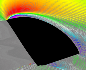
3.2 Time-averaged vorticity field for different wind conditions
Figure 5 shows the near wake of the baseline sail  $S_1$. Time-averaged streamlines and contours of non-dimensional spanwise vorticity $\omega _z {c}/U_\infty$ are presented for two trim angles, ${\eta = 0^\circ }$ and $\eta = -10^\circ$. These two angles are selected because the sail trim that allows $C_{DF,{max}}$ ( $\eta =0^\circ$) is the optimum trim in light wind speed conditions. Conversely, in strong wind conditions, the trim allowing the maximum boat speed is one that provides a reduced side force coefficient ( $C_{SF}$), and thus leeway and heeling angles. Therefore, there is a stronger wind condition, which depends on the hydrodynamic characteristics of the boat, such that the trim allowing the maximum boat speed is $\eta =-10^\circ$. Five flow fields are presented, corresponding to the five PIV measurement planes introduced in figure 2. Regions of no data due to laser shadow are shaded in grey. A total of 500 images are averaged per plane.

Figure 5. Time-averaged near-wake streamlines and non-dimensional vorticity contours of sail  $S_1$ for the optimal sail trim in light wind conditions ( $\eta =0^\circ$, two left columns) and a depowered trim for strong wind conditions ( $\eta =-10^\circ$, two right columns).
The light wind condition  $\eta = 0^\circ$ is shown in the left two columns of figure 5. The streamlines reveal a large time-averaged recirculation region in most of the planes. Because of the lack of the third velocity component, rather than identifying structures with the streamlines, we use the bifurcation lines, nodes and centres as an indication of how two-dimensional or three-dimensional the flow could be, as suggested by Reference Perry and SteinerPerry and Steiner (2001).
Following the definitions of Reference Perry and SteinerPerry and Steiner (2001), we identify bifurcation lines, which are streamlines that converge into a common streamline, and stable foci, which are individual streamlines that spiral inwards and end at a point. Both bifurcation lines and stable foci denote three-dimensional flow. Lastly, we also identify centres, which are closed loop concentric streamlines that are typically found in two-dimensional flow. In figure 5, stable foci are observed at the centre of the circulation regions, indicating the three-dimensionality of the flow field. At the head of the sail at  $\eta =0^\circ$, a bifurcation line appears in plane A at the centre of the recirculation region. Contrarily, near midspan of the sail, such as in plane D and at $\eta = 0^\circ$, two-dimensional centres appear in the recirculation region.
At the strong wind condition  $\eta = -10^\circ$, a stable centre near the surface of the sail is noted on mid-plane C. Conversely, in planes A and B, the streamline patterns close to the surface of the sail are c-shaped and indicative of vortex shedding. Reference Perry and SteinerPerry and Steiner (2001) showed this same pattern in the wake behind a bluff body when the train of leading- and trailing-edge vortices came in close proximity to each other.
We note that a true two-dimensional centre would only exist in a small number of planes (if any) and it is unlikely that the PIV planes of this experiment hit this plane exactly. However, two-dimensional flow is likely to occur between mid-span and 3/4 of the span of the sail (Reference Souppez, Arredondo-Galeana and ViolaSouppez et al., 2019; Reference Viola, Bartesaghi, Van-Renterghem and PonziniViola et al., 2014).
The vorticity contours identify two opposite sign circulation areas in all of the planes and at both  $\eta = 0^\circ$ and $\eta = -10^\circ$, with negative vorticity emerging from the leading edge and positive vorticity from the trailing edge. On planes A, B and C, the positive and negative vorticity of the wake of the post (indicated by a black dot) is also visible on the windward side of the sail section. In the figure, the sail sections are highlighted in red.
At  $\eta = 0^\circ$, flow in planes A, B and C is stalled resulting in a large trailing-edge wake. Conversely, at $\eta = -10^\circ$, these planes experience a three-dimensional flow with vorticity mostly following the sail profile. Flow in planes D and E is stalled at both $\eta$ values.
It is noted that the present results might be partially affected by the limited clearance between the tip of the sail and the side wall of the water tunnel. Whilst the effect of the blockage on the forces is addressed in detail in Appendix A, the effect of the limited tip clearance on the three-dimensionality of the flow is not known. This might include, for example, a reduction of spanwise flow in the near wake.
3.3 Instantaneous vorticity field
The instantaneous vorticity field is investigated with five consecutive images in figure 6, where the first image of each subset is randomly selected from the 500 image data set used in § 3.2. The flow field was sampled at 7.5 Hz, resulting in a non-dimensional period between consecutive images of  ${t^{*} = t U_\infty /{c} = 0.13}$. Each image is labelled with an index $s$ indicating the sequence number of the image. The instantaneous flow fields are shown for planes A–E of geometry $S_1$ at $\eta = 0^\circ$ and $\eta = -10^\circ$. It should be recalled that the five planes were not recorded simultaneously. To identify coherent regions of co-sign rotating flow, the $\gamma _{2}$-criterion (Reference Arredondo-Galeana, Young, Smyth and ViolaArredondo-Galeana, Young, Smyth, & Viola, 2021; Reference Graftieaux, Michard and GrosjeanGraftieaux, Michard, & Grosjean, 2001) is used. The full data set of instantaneous flow fields is available in the supplementary material on the Edinburgh DataShare repository (https://doi.org/10.7488/ds/2857).

Figure 6. Sequence of  $\gamma _{2}$-contours of sail $S_1$ based on vorticity measurements taken at five consecutive acquisition time steps ( $s=1$–5) on planes A, B, C, D and E (columns 1–6, respectively) at $\eta = 0^\circ$ (top array) and $\eta = -10^\circ$ (bottom array). The red crosses indicate sampling points used for the power spectral densities of $\gamma _{2}$ discussed in § 3.3.
A closed  $\gamma _{2}$ isolines formed at the leading and trailing edges are identified as the LEV and trailing-edge vortex (TEV), respectively. Both LEVs and TEVs are continuously generated and shed downstream. The LEV appears to have a more coherent vortex structure than the TEV, which instead shows a more stretched vorticity distribution in the streamwise direction. The LEV convects at approximately $U_\infty /2$. For example, on plane D at $\eta =0^{\circ }$, the streamwise velocity of the LEVs is, on average, $0.53U_\infty$. This is in agreement with the findings of Reference Siala and LiburdySiala and Liburdy (2019), Reference Ōtomo, Henne, Mulleners, Ramesh and ViolaŌtomo, Henne, Mulleners, Ramesh, and Viola (2020) and Reference Smith, Pisetta and ViolaSmith et al. (2021), who found that the LEV convects downstream at approximately the mean shear layer velocity. In fact, assuming that the external shear layer velocity is approximately $U_\infty$, and the internal flow is approximately stagnant, the mean shear layer velocity is $U_\infty /2$. Due to the lower coherence of the TEVs in comparison with the LEVs, we were not able to provide an accurate measurement of their convection velocity. However, we note that studies of lifting surfaces with separated flow on the suction side at similar Reynolds numbers as the ones used in this experiment suggest that the TEV convects approximately at $U_{\infty }$ (Reference Babinsky, Stevens, Jones, Bernal and OlBabinsky, Stevens, Jones, Bernal, & Ol, 2016; Reference Ōtomo, Henne, Mulleners, Ramesh and ViolaŌtomo et al., 2020).
In contrast with some previous observations (Reference Arredondo-Galeana and ViolaArredondo-Galeana & Viola, 2018), a stable LEV with a significant size is not found in any of the measured flow fields. The flow is characterised by a separated shear layer, which has a strong three-dimensional flow component, but is insufficient to stabilise a significant leading-edge vortical structure. This is discussed further in § 3.5, where the vorticity fluxes are quantified. It should be noted, however, that the limited tip clearance might have reduced the spanwise vorticity flux within the core of the LEV, while a sufficient vorticity flux is a necessary condition to enable a stable vortex (Reference MaxworthyMaxworthy, 2007).
3.4 Time-averaged vorticity field for different sails
An overview of the flow and vorticity field was presented in § 3.2, including a comparison between  $\eta =0^{\circ }$ (light wind) and $\eta =-10^{\circ }$ (strong wind conditions). In this section, the effect of the twist is investigated. The three different sails provide a similar maximum driving force. Hence, in spite of the very different twist, all three sails can be considered to be good performance sails. The differences between the maximum driving force coefficients of the three sails are within 1 %, which is significantly smaller than the 25 % difference between the driving force coefficient of $S_1$ between $\eta =0^\circ$ and $-10^\circ$.
Figure 7 shows the streamlines and vorticity contours of the time-averaged flow fields of planes A, B and C for geometries  $S_1$, ${{S_{2}}}$ and $S_3$ at $\eta =0^\circ$. As in figure 5, the bifurcation lines and the stable foci show the three-dimensionality of the flow. This is also shown by the streamlines terminating on the surface of the sail. For each plane, the flow field topologies of the three sails show remarkable similarities despite the significant differences in the angles of attack between each sail. For example, between $S_1$ and $S_3$ there is an angle of attack difference of approximately $5^\circ$ at the top planes of the sails. As shown in table 1, which presents the angles of attack of each plane for the three sails at $\eta =0{^\circ }$, the three sails share the same angle of attack somewhere between plane D and E.

Figure 7. Time-averaged near-wake streamlines and non-dimensional vorticity contours of sails (a)  $S_1$, (b) $S_2$ and ( $3$)
$3$)  $S_3$. Dashed lines $L_1$, $L_2$ and $L_3$ are used in § 3.5 to integrate the vorticity flux. The condition tested for the three sails is $\eta =0^{\circ }.$
Table 1. Angles of attack at the five planes of sails  $S_1$, $S_2$ and $S_3$ at maximum driving force trim $\eta =0{^\circ }$.

At  $\eta =0{^\circ }$, sail $S_3$ has zero twist and an angle of attack of $30^\circ$, which is higher on the highest planes (A–B) and lower on most of the lowest planes (D–E) than the other two sails. Differently from $S_1$ and $S_2$, figure 7 shows that the time-averaged flow field of $S_3$ is attached to planes B and C with the exception of plane A. Conversely, $S_1$ and $S_2$ show trailing-edge separation, resulting in positive vorticity formed on the upper surface of the sail. It is noted that this layer of positive vorticity is above the uncertainty threshold.
These results suggest that the forces of a sail are only marginally affected by whether the time-averaged flow around the sail is mostly attached or separated, and also by the presence of surface positive vorticity, but show instead that forces depend on the overall near-wake vorticity field, which is similar between the three sails.
3.5 Vorticity flux balance
To further characterise the vorticity fields in figure 7, the streamwise vorticity flux was computed across three vertical lines  $L_{1}$, $L_{2}$ and $L_{3}$ positioned near the leading edge, mid-chord and near the trailing edge, respectively, of each of the evaluated sail sections of figure 7. Lines $L_{1}$, $L_{2}$ and $L_{3}$ start on the surface of the sail and end at the upper boundary of each panel. This ensures that the full width of the leading-edge shear layer is included in the flux computation. As such, the vorticity fluxes are computed as
 \begin{equation} \int_L u_x \omega_z \,{{\rm d} y}, \end{equation}
for  $L=L_1, L_2$ and $L_3$, respectively. Results are shown in figure 8.

Figure 8. Non-dimensional streamwise fluxes of spanwise vorticity across lines  $L_1$ (leading edge), $L_2$ (mid-chord) and $L_3$ (trailing edge) of planes A, B and C of (a) $S_1$, (b) $S_2$ and (c) $S_3$ at $\eta =0^\circ$.
Because of the leading-edge separation, most of the negative vorticity is generated at the leading-edge shear layer ( $L_1$). Figure 8 shows that at $L_1$, the magnitude of the flux increases from $S_1$ to $S_2$ and to $S_3$. This is due to an increase in the angle of attack. In fact, the vorticity production rate is expected to increase when the angle of attack approaches ${\rm \pi} /2$ from lower values (see, for instance, figure 3 in Reference DeVoria and MohseniDeVoria & Mohseni, 2017).
The magnitude of the flux decreases from  $L_{1}$, $L_{2}$ and $L_{3}$ for each sail. This suggests that the vorticity is either annihilated by surface positive vorticity or convected out of the plane. However, annihilation by surface positive vorticity can be excluded because this decreasing trend is also clearly visible on plane C of $S_3$, where there is no surface positive vorticity. Hence, the production of surface positive vorticity is comparatively small and unlikely to play a role in the force production mechanisms.
Because vorticity is divergence free ( $\boldsymbol {\nabla } \boldsymbol {\cdot } \boldsymbol {\omega }=0$), the decay of negative spanwise vorticity produced at the leading edge must be balanced by the generation of streamwise vorticity in the absence of dissipation. In fact, using Einstein notation, the vorticity transport equation for the spanwise component of vorticity is
 \begin{equation} \frac{\partial \omega_z}{\partial t} + u_j \frac{\partial \omega_z}{\partial x_j} = \omega_j \frac{\partial u_z}{\partial x_j} + \nu \frac{\partial^2 \omega_z}{\partial x_j \partial x_j}, \end{equation}
where  $u_j$ and $\omega _j$ are the $j$th component of the velocity $\boldsymbol {u}=(u_x,u_y,u_z)$ and of the vorticity $\boldsymbol {\omega }=(\omega _x,\omega _y,\omega _z)$, respectively; $t$ is time and $\nu$ is the kinematic viscosity. We neglect the unsteady term (i.e. the first term) on the left-hand side of (3.3) because we found that it is less than 5 % of the advection term (i.e. the second term). Neglecting also viscous diffusion, (3.3) becomes
 \begin{equation} u_j \frac{\partial \omega_z}{\partial x_j} = \omega_j \frac{\partial u_z}{\partial x_j}. \end{equation}
 Equation (3.4) is integrated on a control volume with unit spanwise thickness between  $L_1$ and $L_3$, the sail surface and the upper boundary of the field of view, and whose external surface is $C$.
$C$.
By using the divergence theorem, the integrated equation becomes
 \begin{equation} \int_C n_j u_j \omega_z \, \mathrm{d}C = \int_C n_j \omega_j u_z \, \mathrm{d}C, \end{equation}
where  $n_j$ is a unit vector orthogonal to $C$ and pointing outward. The left-hand side is the net spanwise vorticity flux through the surface of the control volume, whilst the right-hand side is the vortex tilting in the $x$- and $y$-directions, respectively, and the vortex stretching in the $z$-direction. This vorticity balance equation can be further simplified by noting that, on the plane orthogonal to $z$, the vortex stretching perfectly balances the net flux of spanwise vorticity, because $n_j u_j \omega _z - n_j \omega _j u_z = u_z \omega _z - \omega _z u_z=0$. Because the $y$-dimension of the control volume is sufficiently large, the vorticity vanishes on the upper $y$-normal face of $C$ and the velocity vanishes on the lower surface bounded by the sail. Then, the vorticity transport equation states that the net spanwise vorticity flux along the $x$-direction of the control volume is balanced by vortex tilting in the same direction (Reference Milne-ThomsonMilne-Thomson, 1973)
 \begin{equation} \int_{C_x} u_x \omega_z \, \mathrm{d}C_x = \int_{C_x} \omega_x u_z \, \mathrm{d}C_x. \end{equation}
Reformulating (3.6) per unit depth, it becomes
 \begin{equation} \int_{L_3} u_x \omega_z \, \mathrm{d} y -\int_{L_1} u_x \omega_z \, \mathrm{d} y = \int_{L_3} \omega_x u_z \, \mathrm{d} y. \end{equation}
This shows that the decay of negative spanwise vorticity observed in figure 8 is due vortex tilting in the streamwise direction.
4. Discussion and conclusions
The vortex flow of spinnaker sails is investigated by testing three model-scale sails with different twist profiles at various trim angles in a water tunnel. At any horizontal sail section, the flow separates at the leading edge and a turbulent shear layer develops downstream of the leading edge. Depending on the angle of attack of the sail section, time-averaged flow reattachment can occur.
Vorticity shed from the leading-edge shear layer forms coherent LEVs that are identified with a  $\gamma _2$ vortex detection algorithm. Despite the relatively high $\varLambda$ ( $35^{\circ }$), which is indicated in figure 1(a), no evidence is found of an attached LEV that remains stably attached as, for instance, occurs on a delta wing. In contrast, LEVs convect downstream at half of the free-stream velocity, which is approximately the mean shear layer velocity. Vorticity shed by the trailing edge forms smaller and less coherent TEVs (whose velocity could not be quantified). Reducing $\eta _{0}$ by $10^\circ$, results in drops of the driving and side forces of 17 % and 30 %, respectively.
The main finding of this work is that the slope of the lift with the angle of attack is independent of the sail twist, despite the significantly three-dimensional flow field around the sail. At the sail trim corresponding to the maximum driving force, the sail is either stalled or experiences leading-edge separation followed by flow reattachment depending on the twist. Remarkably, both of these conditions result in a similar force because the overall vorticity field is only marginally affected by the local flow reattachment.
Stalled sails generate surface counter-rotating vorticity, but this vorticity is negligible compared with the free vorticity in the near wake. Changes in the vorticity fluxes are found to be governed by vortex tilting rather than vortex annihilation.
Because the point of flow separation is fixed at the leading edge, these general conclusions are expected to be valid also at the higher Reynolds numbers of a full-scale sail. However, we speculate that, while the reattached boundary layer in recirculating regions is likely to relaminarise in the experiments, see for example the findings on the flow past circular arcs by Reference Souppez, Bot and ViolaSouppez et al. (2022), relaminarisation is unlikely to occur at full scale.
The spinnaker was tested in isolation, without the hull and the mainsail. It is expected that the effect of the hull would be significant mostly on the lowest sections of the spinnaker and would not change the conclusions of this work. The mainsail circulation should result in a higher average angle of attack on the spinnaker. Consequently, with the mainsail, the sail trim that maximises the thrust would be at  $\eta <0^{\circ }$ and less flow separation might occur. Furthermore, if there is sufficient overlap between the two sails, the direction of the mainsail-induced velocity near the spinnaker's trailing edge might promote flow reattachment. Hence, while the present conclusions are expected to hold also at higher Reynolds numbers and in the presence of the mainsail, the measured flow separation could be overestimated.
Supplementary material
Supplementary material are available at https://doi.org/10.1017/flo.2023.1. Spinnaker geometries are available at Edinburgh DataShare: https://doi.org/10.7488/ds/2857.
Acknowledgements
The authors would like to thank J.-B. Souppez and S. Ōtomo for the valuable discussions that contributed greatly to this study, as well as the three anonymous reviewers, whose comments substantially helped improve the quality of this manuscript.
Funding statement
This work received funds from the Consejo Nacional de Ciencia y Tecnología (CONACYT) through the grant number 384490.
Declaration of interests
The authors declare no conflict of interest.
Author contributions
A.A.G. designed the experiments, undertook the measurements and the data analysis and wrote the first draft of the manuscript. H.B. contributed to the interpretation and presentation of the results, reviewed and edited the manuscript. I.M.V. conceived and supervised the project, reviewed and edited the manuscript.
Ethical standards
The research meets all ethical guidelines, including adherence to the legal requirements of the study country.
Appendix A. Blockage effects
Force corrections are applied for solid, wake blocking and streamline curvatures (Reference Barlow, Rae and PopeBarlow, Rae, & Pope, 1999). The force correction factor is reduced to  $1-2\epsilon$, since the boundary layer correction factor is taken to be that of a jet with horizontal boundaries, with a jet width to height ratio ( $r$) equal to $r=1$, hence $\delta _{{b}} = 0$. For unusual shapes $\epsilon$ is
 \begin{equation} \epsilon = \dfrac{A_{m}}{4A_{t}}, \end{equation}
where  $A_{m}/A_{t}$ is the blockage ratio. Three blockage ratios were computed at three rotation angles $\eta$, where $\eta =-20^\circ$, $\eta =0^\circ$ and $\eta =5^\circ$, correspond to the positions where maximum lift to drag ratio, maximum driving force and maximum lift were recorded for sail $S_1$.
To ensure that the blockage correction is accurate, experimental data of blockage corrections of a thin circular arc were used for comparison. This is a geometry which is similar to the mid-height section of the scale model spinnakers. The experimental data were provided by Reference Souppez, Arredondo-Galeana and ViolaSouppez et al. (2019) and measured in the towing tank of Solent University at  $Re = 150\ 000$. The experiments were designed to measure the blockage effect on a finite-aspect-ratio circular arc at angles of attack of $15^\circ$ and $20^\circ$. The chord of the arc was $0.1\ \mathrm {m}$ and the span $0.37\ \mathrm {m}$. Different blockage ratios were tested, by adjusting two sidewalls to each side of the arc. Figure 9 shows the ratio of the corrected lift coefficient to the uncorrected lift coefficient ( $C_{L}/C_{L,u}$) plotted against blockage ratio ( $A_{m}/A_{t}$).

Figure 9. Blockage corrections measured at Solent University at  $Re=150\ 000$ for a circular arc of ${{A{\kern-4pt}R} }=3.7$, at $\alpha =15^\circ$ (+), $\alpha =20^\circ$ (*, red) and correction $1-2\epsilon$ (x, blue), as applied in this work for $\eta =-20^\circ$, $\eta =0^\circ$ and $\eta =5^\circ$.
Three cases are presented. The black and red markers, correspond to the tests at Solent University at  $Re = 150 \ 000$ for blockage ratios of $0.020,0.062,0.130$ and $0.022,0.071,0.153$, tested at $\alpha = 15^\circ$ and $\alpha = 20^\circ$, respectively. The blue markers represent the correction from Reference Barlow, Rae and PopeBarlow et al. (1999). This correction is applied to the lift coefficients of the sail measured at $\eta =-20^\circ$, $\eta =0^\circ$ and $\eta =5^\circ$ and is equal to $1-2\epsilon$, where $\epsilon$ is calculated from (A1). Figure 9 shows a satisfactory agreement between $1-2\epsilon$ and the Solent University tests. Two linear fits of the Solent University data for $\alpha =15^\circ$ and $20^\circ$ are shown in figure 9. The distance between these lines is smaller than 8 % at $A_{m}/A_{t} = 0.20$. The correction applied in this work fits between these regression lines and hence the error in the blockage correction is estimated to be smaller than 8 %.


 Open access