


1. Introduction
The Ross Sea plays a major role for the Southern Ocean sea-ice cover and mass and for the formation of the dense water that contributes to the Antarctic Bottom Water (AABW). the oceanographic conditions in the southwestern Ross Sea are relatively well studied (Reference Jacobs, Amos and BruchhausenJacobs and others, 1970; Reference Jacobs and ComisoJacobs and Comiso, 1989). One relevant part of these conditions is water-mass modification triggered by polynya events and the associated cooling and brine enrichment of the water masses by ice formation (Reference LemkeLemke, 2001). In particular the coastal polynyas that form in Terra Nova Bay (TNB) and along the Ross Ice Shelf (RIS) (Reference Bromwich and KurtzBromwich and Kurtz, 1984; Reference Jacobs and ComisoJacobs and Comiso, 1989; Reference Van WoertVan Woert, 1999) are known as so-called ice factories. the TNB polynya (TNBP) is a coastal polynya bounded by steep glacier valleys and terminating in the Drygalski area. the RIS polynya (RISP) forms in the lee of the floating ice shelf (Reference Jacobs and ComisoJacobs and Comiso, 1989; Reference Petrelli, Bindoff and BergamascoPetrelli and others, 2008). Both are relevant in the production of water masses that are precursors of AABW (e.g. Reference Van WoertVan Woert, 1999; Reference Tamura, Ohshima and NihashiTamura and others, 2008).
Estimates of polynya area and the associated ice production have been sparse until recently (Reference Martin, Drucker and KwokMartin and others, 2007; Reference Tamura, Ohshima and NihashiTamura and others, 2008; Reference KernKern, 2009) and all of these used data from satellite microwave radiometry in combination with numerical weather prediction model data (reanalysis).
Here we show a comparison of oceanographic data (temperature, salinity and currents) obtained in 1996 and 1997 in TNB (mooring D), the polynya area and estimates of the associated ice production rates for the TNBP for the same years. Based on lag correlation analysis, the relationships between polynya area and ice production on the one hand and changes in the temperature and salinity observations on the other hand are examined. the water-current time series aid in the interpretation of the results.
2. Circulation of the Western Ross Sea and the Terra Nova Bay Area
Large-scale ocean circulation in the western Ross Sea is characterized by a cyclonic gyre and involves the following water masses: Antarctic surface water (AASW), ice-shelf water (ISW), modified Circumpolar Deep Water (mCDW) and high-salinity shelf water (HSSW) (Reference Jacobs, Fairbanks, Horibe and JacobsJacobs and others, 1985). Surface waters in the southern Ross Sea flow westward along the RIS. In McMurdo Sound (McMS) a cyclonic surface circulation can be found. Abrupt changes in temperature recorded in this circulation by Reference Hunt, Hoefling and ChengHunt and others (2003) can be associated with intrusions of mCDW. Then the currents flow out of McMS northwards along Victoria Land (Reference Barry and DaytonBarry and Dayton, 1988).
mCDW is usually found at intermediate depths extending from the northern Ross Sea southward into the cavity beneath the RIS. Its salinity is centred around 34.54 and its temperature is near –1˚C. It evolves into AASW after its upwelling and modification by interaction with the atmosphere (Reference Jacobs, Fairbanks, Horibe and JacobsJacobs and others, 1985). Deep water exits the Ross Sea as bottom currents, at Cape Adare as HSSW and around dateline meridian as ISW.
TNB is located in the southwestern Ross Sea. It is about 64 km long and is located between Cape Washington and the Drygalski Ice Tongue along the coast of Victoria Land (Fig. 1). Its southern border is protected from incoming sea ice by the Drygalski Ice Tongue, the length of which can control the polynya size (Reference FrezzottiFrezzotti and Mabin, 1994). the western border is the Hell’s Gate area which is a key site for the polynya area dynamics determined by the ubiquitous katabatic winds that open the polynya and trigger surface water cooling and dense water formation via ice production (Reference Bromwich and KurtzBromwich and Kurtz, 1984).
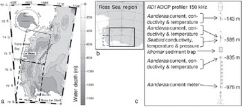
Fig. 1. (a) Bathymetry of the western Ross Sea and the location of mooring D. For dotted and dashed boxes see (b); the inset denotes the location of the region with respect to Antarctica. (b) Location and extent of the Ross Sea region (grey area) onto which the Polynya Signature Simulation Model is applied. the dotted, dashed and solid boxes denote the regions TNBP, McMS and RISP, respectively. (c) Sketch of mooring D during its deployment in 1996/97. ADCP is acoustic Doppler current meter.
The vertical structure of the water column in TNB is relatively simple (Reference Budillon and SpezieBudillon and Spezie, 2000). the greatest variability is in the surface layer that extends to 50–150m depth (Reference Gordon, Codispoti, Jennings, Millero, Morrison and SweeneyGordon and others, 2000). the water column below is nearly isothermal; its vertical stability is preserved by the increasing salinity. the vertical structure of the summer water column in TNB may therefore be considered as two-layered. This is illustrated in Figure 2, showing the vertical distribution of the potential temperature interpolated from ship-based in situ measurements in late summer 1995 (see also Reference Manzella, Meloni, Picco, Spezie and ManzellaManzella and others, 1999), 1996 and 1997. the summer surface water (SSW) occupies the upper layer that becomes fresher and warmer because it is influenced by summer sea-ice melting and by the heat gain from solar radiation that is the main constituent of the surface heat balance in summer in this region (Reference Budillon, Fusco and SpezieBudillon and others, 2000). Below this layer, the water column comprises HSSW with a potential temperature close to the surface freezing point and salinity above 34.7.
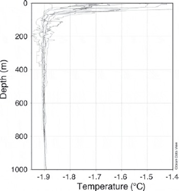
Fig. 2. Vertical profiles of the potential temperature from ship-based in situ measurements in TNB within 200km of the location of mooring D during 18–20 February 1995, 28 January–9 February 1996 and 22–27 December 1996.
Once formed, HSSW splits into two parts, one of which flows northwards and off the shelf while the other flows southwards intruding below the RIS. the latter gives origin to the thermohaline process culminating in the formation of ISW (Reference MacAyealMacAyeal, 1984). A quasi-isothermal water mass with temperatures below the surface freezing point (Tf = –1.914˚C for P = 0 dbar and S = 34.85) was detected at intermediate depths. This layer is called TISW (Terra Nova Bay ice-shelf water) and has been observed over the whole area of TNB at different depths and thickness (Reference Budillon, Fusco and SpezieBudillon and others, 2000; Reference Budillon and SpezieBudillon and Spezie, 2000; Reference Van WoertVan Woert and others, 2001). Apart from this, our knowledge about the circulation of water masses within the TNBP is scant.
3. Data
3.1. In situ observations
A number of moorings were deployed as part of the longterm monitoring of Ross Sea circulation by the Italian PNRA (Programma Nazionale di Richerche in Antartide) project CLIMA. One of them, mooring D, was and still is located in TNB, and since 1995 (Reference Manzella, Meloni, Picco, Spezie and ManzellaManzella and others, 1999) has been continuously recording sea-water temperature, conductivity and currents. In this study, we use data of mooring D positioned from 1995 to 1997 at 75˚07.145’ S, 164˚13.295’ E at a water depth of 998 m. the location of the mooring is shown in Figure 1a; a sketch of the mooring as deployed in 1996/97 is given in Figure 1c. the mooring was deployed on 1 February 1996 and recovered on 8 December 1997 after 2 years at sea. Measurement depths for the aforementioned parameters are 143, 585, 835 and 979m as indicated in Figure 1c. In this study we use only data (currents speed and direction, temperature, and conductivity) obtained with the Aanderaa (model RCM7) current meters. Their accuracy is ±1cms–1 in speed and ±5˚ in direction. These current meters also included built-in sensors: a Fenwall GB32JM19 temperature sensor with an accuracy of 0.1˚C and a conductivity cell with an accuracy of 0.007 Sm–1. All instruments were factory-calibrated. A post-deployment check was performed which included comparing in situ performance against conductivity–temperature–depth (CTD) casts by SBE 911 probe on board ship before and after deployments. Instrumental errors had been checked. the dataset used in this study spans the years 1995–97.
The temperature and conductivity data from instruments at 143 mdepth were compared with satellite data. Data from all depths were used to improve the knowledge of the circulation pattern and hydrology already available in the literature (Reference Manzella, Meloni, Picco, Spezie and ManzellaManzella and others, 1999; Reference Picco, Amici, Langone, Ravaioli, Spezie and ManzellaPicco and others, 1999).
Potential temperature plots were achieved after a reelaboration of the CTD data from the cruises of the CLIMA project already reported in the literature (Reference Fonda UmaniFonda Umani and others, 2005; Reference Petrelli, Bindoff and BergamascoPetrelli and others, 2008). Figure 2 reveals that the measurements of the oceanic parameters at 143 m depth are representative of the water-mass properties just below the summer water layer (of SSW).
3.2. SSM/I PSSM polynya area
Brightness temperatures measured by the polar orbiting Special Sensor Microwave/Imager (SSM/I) were used to derive the polynya area using the Polynya Signature Simulation Method (PSSM). the PSSM was developed by Reference Markus and BurnsMarkus and Burns (1995) and refined by Reference Hunewinkel, Markus and HeygsterHunewinkel and others (1998). the method is based on polarization ratios (i.e. vertically minus horizontally polarized brightness temperature divided by their sum) observed by the SSM/I at 37.0 and 85.5 GHz. It combines the finer spatial resolution at 85.5 GHz (field-of-view 13 km×15 km; sampling distance 12.5 km) with the lower weather influence at 37.0GHz (field-of-view 29 km×37 km; sampling distance 25 km) in an iterative approach in which the spatial distribution of three surface classes (open water, thin ice, thick ice) is obtained. This distribution gives the areas of open water and thin ice, which are together considered as the polynya area. the polynya area can be estimated with a mean accuracy of ±80 km2. Changes in the area of ±50km2 are observable (Reference Markus and BurnsMarkus and Burns, 1995; Reference Hunewinkel, Markus and HeygsterHunewinkel and others, 1998) provided that the SSM/I data are interpolated onto a grid with 12.5 km×12.5km (37.0 GHz) and 5 km ×5 km (85.5 GHz) grid resolution. the PSSM was applied in a number of studies (e.g. Reference Markus, Kottmeier, Fahrbach and JeffriesMarkus and others, 1998; Reference Martin, Polyakov, Markus and DruckerMartin and others, 2004) and was modified to derive a circum-Antarctic polynya-area time series (Reference Kern, Spreen, Kaleschke and HeygsterKern and others, 2007; Reference KernKern, 2009). In this study, PSSM retrievals of the polynya area of the Ross Sea region are used. Figure 1b shows the area covered by the Ross Sea region together with sub-regions TNBP, McMS and RISP used to calculate the polynya area and associated ice production further investigated in this study.
Figure 3 shows a sample set of PSSM-based polynya distribution maps used as input in this study. Since these maps are obtained using SSM/I swath data, several maps are available each day. We used data from 1996 and 1997, from April to September.
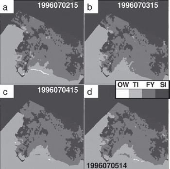
Fig. 3. Sample set of PSSM-based polynya area (open-water plus thin-ice area) distribution in the Ross Sea region (see Fig. 1b) derived from SSM/I swath data for 2–5 July (days 183–186) 1996. Ice types are denoted according to the legend, where OW, TI, FY and SI denote open water, thin ice, ‘regular’ first-year ice and ‘stable’ first-year ice, respectively (see Reference Kern, Spreen, Kaleschke and HeygsterKern and others, 2007).
In order to obtain the polynya area, all gridcells (grid resolution 5 km ×5 km) which show either open water or thin ice were summed and multiplied by the area of the gridcell. Figure 4 shows the time series of the polynya area for region TNBP for 1996 and 1997.
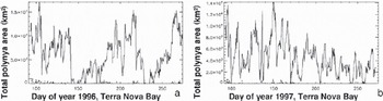
Fig. 4. Time series of the daily polynya area as derived with the PSSM for region TNB for (a) 1996 and (b) 1997. Note the different y-axis scaling.
The ice production as associated with the observed polynyas was calculated as follows. European Centre for Medium-Range Weather Forecasts (ECMWF) re-analysis (ERA-40) data (air temperature and humidity, wind speed, surface pressure) (Reference Kållberg, Simmons, Uppala and FuentesKållberg and others, 2004) were interpolated onto the same grid as was used for the PSSM. Calculations were done for April–September to minimize the influence of solar radiation, which we neglect here. the net surface heat flux, Ft, then comprises the net longwave heat flux and the turbulent fluxes of sensible and latent heat (e.g. Reference Van WoertVan Woert, 1999).
Fs, Fl, Fup and Fdown are the sensible, latent, longwave emitted and longwave downwelling fluxes, respectively. the sensible and latent heat fluxes are calculated using common bulk formulae:
where ρair = 1.3 kgm–3 is the density of cold air, cp = 1004 J kg–1 K–1 is the specific heat of dry air, Cs = 0.0018 is the bulk transfer coefficient for heat/moisture (at 2m height), u is the wind speed at 2 m height, L = 2.5×10⁶ J kg–1 is the latent heat of evaporation, Tair is the air temperature at 2m height, Ts is the surface temperature and set to the temperature of freezing sea water (–1.8˚C), q is the specific humidity at 2 m height and qs is the specific humidity at the surface.
The value used for Cs differs from values reported in the literature and used for similar purposes. Reference Drucker, Martin and MoritzDrucker and others (2003) and Reference Yu and LindsayYu and Lindsay (2003) used a value of 0.003, which was deduced from in situ measurements over narrow leads (Reference Lindsay and RothrockLindsay and Rothrock, 1994). This value is, however, valid for a height above ground of 10 m and a temperature difference between the surface and the air of at least 10 K. Reference Andreas, Paulson, Williams, Lindsay and BusingerAndreas and others (1979) and Reference Andreas and MurphyAndreas and Murphy (1986) defined the bulk transfer coefficient over Arctic leads to be 0.0021–0.0025 at a height of 2 m a.s.l., but only 0.0013 at 10m height. Over open water they defined Cs as being 0.001. In this study, the calculations are carried out for a height of 2 m above the ground, so values like 0.003 and/or 0.0021–0.0025 seem to be appropriate, though only for small leads/polynyas and a large temperature difference. To account for the fact that the polynyas considered in this study are relatively large and cannot be compared to a narrow lead, a value between that used for open water and those found for narrow leads is chosen: 0.0018.
The wind speed in the ERA-40 data is given for a height of 10 m above the ground. Using the wind-profile power law relationship the wind speed at 2 m height above ground can be approximated as u 2m = u 10m /50: 1(Reference StullStull, 1988; Reference EtlingEtling, 1996); an exponent of 0.1 is valid for labile conditions encountered in a polynya. the specific humidity was calculated via computation of the partial water vapour pressure from the dew-point temperature using the Clausius– Clapeyron formula using coefficients valid for saturation with respect to ice. the relative humidity directly above the water surface can be assumed to be 100%. Therefore the partial water vapour pressure directly above a water surface at its freezing point (in our case T s = –1.8˚C) can be set to the saturation water vapour pressure.
For the net longwave heat flux, F ud, the parameterization of Reference Berliand and BerliandBerliand and Berliand (1952) was used:
Here ε = 0.98 is the longwave emissivity, σ = 5.67 × 10⁻⁸Wm–2 K–4 is the Stefan–Boltzmann constant, T is the air temperature at 2 m height, C is the cloud coverage and e 0 is the saturation water vapour pressure at the surface. Subsequently the ice production rate was calculated from the net total surface heat flux using:
where the ice production rate P ice is the total net heat flux F t divided by the density of the ice (frazil ice), ρ ice = 950 kgm–3, and the latent heat of fusion, L h = 334 kJ kg–1.
The above-mentioned formulae were used to calculate the daily mean ice production rate for the entire Southern Ocean. In the following step the PSSM-based polynya-area distribution maps were used to calculate the mean daily ice production only for the mean daily polynya areas in regions TNBP, RISP and McMS. In other words, only those gridcells that belong to polynyas were used to calculate the total mean ice production. This assumes, however, that the entire polynya area obtained with the PSSM is open water. This is not true. the open-water fraction is <100%. Therefore, to avoid an overestimation of the ice production (km3 d–1), the ice production rate P
ice was weighted with values of the mean ice concentration for the two polynya surface classes – open water (C
ow = 25%) and thin ice (C
ti = 65%) – which are close to those reported in Reference Kern, Spreen, Kaleschke and HeygsterKern and others (2007): ![]() N is the number of seconds per day and A
ow and A
ti are the total mean daily areas of the open-water fraction and the thin-ice fraction within the polynya within the respective region. Ideally one should have used values for C
ow and C
ti that were derived directly for the TNBP. However, the TNBP is so small that a comparison between the PSSM polynya area based on SSM/I data and independent high-resolution ice concentration data would not make sense. Reference Kern, Spreen, Kaleschke and HeygsterKern and others (2007) gave two pairs of values: one for the RISP and one for the Mertz Glacier polynya (MGP). In terms of polynya area (development) and in terms of the ice which borders the polynya, the TNBP is more similar to the MGP than to the RISP. Therefore the values chosen are close to those found for the MGP; if we had used the values found for the RISP then the ice production derived in this study for the TNBP would have been smaller.
N is the number of seconds per day and A
ow and A
ti are the total mean daily areas of the open-water fraction and the thin-ice fraction within the polynya within the respective region. Ideally one should have used values for C
ow and C
ti that were derived directly for the TNBP. However, the TNBP is so small that a comparison between the PSSM polynya area based on SSM/I data and independent high-resolution ice concentration data would not make sense. Reference Kern, Spreen, Kaleschke and HeygsterKern and others (2007) gave two pairs of values: one for the RISP and one for the Mertz Glacier polynya (MGP). In terms of polynya area (development) and in terms of the ice which borders the polynya, the TNBP is more similar to the MGP than to the RISP. Therefore the values chosen are close to those found for the MGP; if we had used the values found for the RISP then the ice production derived in this study for the TNBP would have been smaller.
Table 1 summarizes the values of the total ice production derived for the three regions TNBP, McMS and RISP for the years 1996 and 1997 for April–September. A conservative error estimate for the given values is between 20% (for the RISP) and 50% (for the TNBP). the larger error for the TNBP is caused by the fact that this polynya is: (1) much smaller and thus the relative error in the polynya area is larger; and (2) much more influenced by katabatic winds which are not resolved by the ERA-40 data used here (e.g. Reference Petrelli, Bindoff and BergamascoPetrelli and others, 2008). In accordance with Reference Petrelli, Bindoff and BergamascoPetrelli and others (2008) we suggest that the values given in Table 1 are an underestimation of the actual conditions, particularly for the TNBP. Other studies reported higher values for the ice production in the two years considered and in general (see Table 1; e.g. Reference Van WoertVan Woert, 1999; Reference Martin, Drucker and KwokMartin and others, 2007; Reference Tamura, Ohshima and NihashiTamura and others, 2008). Note that we used normalized ice production anomalies rather than absolute values in the further analysis and thus the large error in the total ice production values stated here is not important.
Table 1. Total ice production (km3) associated with the PSSM-based polynya area for regions TNBP, RISP and McMS for 1996 and 1997 for months April–September. Numbers in parentheses are values estimated for April–September from Reference Martin, Drucker and KwokMartin and others (2007). Numbers in brackets are values estimated for the entire year from Reference Tamura, Ohshima and NihashiTamura and others (2008). the mean annual value for 1992–2001 is 390 ±59 km3 for the RISP and 59 ±10 km3 for the TNBP according to Reference Tamura, Ohshima and NihashiTamura and others (2008). According to Reference Van WoertVan Woert (1999), May– August ice production in the TNBP was approximately 50 km3 in the years 1988–90
4. Data Comparison
For the comparison of both datasets the mean daily polynya area and associated ice production were interpolated onto the times at which mooring data are available (3 hourly values). Subsequently, a polynomial fit function was used to remove the seasonal cycle in the mooring data and to compare anomalies of the mooring data with anomalies in polynya area and ice production. Figure 5 shows the time series of the anomalies of salinity, temperature, polynya area and ice production together with the u- and v-component of the observed currents for TNB for 1996 (Fig. 5a–f) and 1997 (Fig. 5g–l).
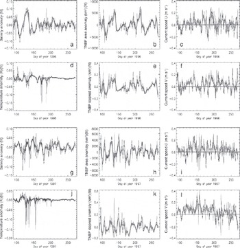
Fig. 5. Time series of the anomalies of salinity and temperature (a, d, g, j) and of polynya area and ice production (b, e, h, k), and time series of the u- and v-components of the ocean currents (c, f, i, l) in region TNB. Thin black (thick grey) lines denote 3 hourly (7 day moving average) values.
Using these anomalies a lag correlation was carried out for (1) the entire time series (April–September, i.e. approximately day of year 91–270); and (2) a 91 day window moved at a step of 30 days, i.e. the sub-periods consisting of days 91–180, 120–210, 150–240 and 180–270. the lag correlation analysis was carried out between the time series of the mooring data (anomalies of salinity and temperature, and the u- and v-component of the currents speed at 143 m depth) and the polynya-area and ice-production anomalies. the time series were smoothed with different running means (1, 3, 5 and 7 days) to investigate the dependency of obtained magnitude and lag of the correlations with regard to the used smoothing window, as we suspect that the unsmoothed time series will be too noisy to obtain a meaningful correlation. the maximum lag used here is 20 days or 160 data points. the significance of the obtained correlations was checked by calculating lag correlations between the dependent (e.g. polynya area) and 1000 randomly shuffled independent time series (e.g. salinity). We also checked the significance of the obtained time lag by calculating the lag correlations with 1000 randomly shuffled time lags.
Selected results of this lag correlation analysis are shown in Figure 6 for the correlation coefficients obtained when comparing polynya area with the observed salinity and temperature in the TNBP. Figure 6a reveals that, taking the entire period into account, a significant correlation exists between polynya area and salinity anomalies observed at mooring D. the same statement can be made for the associated ice production (not shown). Note, however, that this applies primarily for 1996 and not for 1997; in 1997 the correlation seems to be significant as well but much smaller compared with 1996 (Fig. 6e). With a value of the correlation coefficient of 0.7, almost 50% of the variance in the observed salinities seems to be explained by the polynya area anomalies and the associated ice production in the TNBP at a lag of about 4 days (area) and 2–3 days (ice production, not shown) in 1996. the salinity anomalies lag behind area and/or ice production anomalies. A similar statement can be made for the McMS polynya and RISP region (not shown). However, in these regions correlation coefficients are smaller and the time lag is longer, particularly for the ice production.
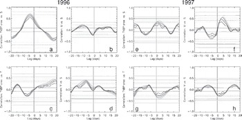
Fig. 6. Time series of lag correlation coefficients between polynya area anomalies and anomalies of the observed salinity (a, e) and temperature (c, g), and between current-speed anomalies and salinity anomalies (u-component: (b, f); v-component: (d, h)). Grey tones and widths of the graphs denote smoothing of the data over 1, 3, 5 and 7 days prior to the analysis from thin and black to bright and light grey, respectively. the horizontal dotted, dashed and solid lines denote significance levels 90% (p = 0.1), 95% (p = 0.05) and 99% (p = 0.01), respectively, for 3 day (dark grey) and 7 day (light grey) smoothing.
Figure 6c and g reveal that the correlation between polynya area and temperature anomalies is small, especially in 1996, and at a longer time lag. the correlation between the observed u- and v-component at the mooring and the observed salinity is small in 1996 (Fig. 6b and d) and for the v-component in 1997 (Fig. 6h), while it peaks at 0.55 (p = 0.05) in 1997 for the u-component (Fig. 6g). Note, however, that here positive (negative) salinity anomalies lead positive (negative) currents anomalies, for example currents with an eastward (westward) component.
Table 2 summarizes the peak correlation coefficients and associated time lags for the TNBP considered for two different smoothing windows for 1996 and 1997. Peak correlations increase with increasing smoothing window length. A smoothing window larger than 7 days did not improve the results further.
Table 2. Peak values of lag correlation coefficients and the associated time lag in days between polynya area anomalies and salinity (italic) or temperature (roman) anomalies for 3 day and 7 day smoothing for the TNBP. A positive (negative) coefficient denotes (anti-) correlation. A negative (positive) time lag means that the polynya area anomaly leads (lags) the salinity and/or temperature anomaly. Numbers given in parentheses denote the p value of the significance test, with 0.10 (0.05) denoting a significance of the correlation of 90% (95%)
Figure 7 shows how the magnitude of the lag correlation between polynya area anomaly and salinity anomaly evolves over the course of the freezing season when using different 90 day time periods. For Figure 7a, only data of days 91–180 are used, for Figure 7b those of days 121–210 and so on. Figure 7 reveals that the magnitude of the correlation decreases with time for the polynya area. the same is true for the ice production (not shown). Table 3 summarizes the peak correlation coefficients for all three regions for the 7 day smoothing for the entire period (days 91–270; see Fig. 6) together with those obtained for the four 90 day sub-periods given in Figure 7, using polynya area and salinity anomalies. It can be seen that only for region TNBP does the correlation remain above 0.5 and significant at 90% in all sub-periods.
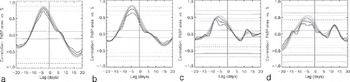
Fig. 7. Time series of lag correlation coefficients between polynya area anomalies and salinity anomalies for the TNBP for 1996 for four different 90 day periods: (a) days 91–180, (b) days 121–210, (c) days 151–240 and (d) days 181–270. See Figure 6 for meaning of different grey values and horizontal lines.
Table 3. Peak values of the lag correlation coefficient between polynya area anomalies and salinity anomalies for 7 day smoothing for 1996 for the entire period (days 91–270) and the different sub-periods described in the text (see also Fig. 7)
The results shown in Figures 5–7 and Tables 2 and 3 are discussed in section 5.
5. Interpretation and Discussion of the Results
Figure 5 and Table 2 reveal two very different conditions: in 1996 positive polynya-area (and ice-production) anomalies led positive salinity and negative temperature anomalies at the mooring position in TNB by about 3–4 days. the significant correlation explained almost 50% of the observed variability in the salinity in the case of the TNBP. This seems reasonable and can be explained by water-mass cooling and ice production associated with the TNBP. In contrast, in 1997, correlations between polynya-area and ice-production anomalies in the TNBP and salinity and temperature anomalies at the mooring position were much weaker and exhibited a ‘wrong’ time lag, with salinity and temperature anomalies leading polynya-area and ice-production anomalies. However, the sign of the correlation was the same in both years. This indicates that a larger (smaller) polynya area and associated ice production seems to be related to a positive (negative) salinity anomaly at the mooring position. Since the mooring is often well inside the polynya, a direct link between polynya activity and water-mass property (salinity, temperature) is to be expected.
Is the observed time lag of 3–4 days reasonable? Although vertical velocities of convection elements in a polynya can be as large as several centimetres per second (Reference FosterFoster, 1972; Reference RudelsRudels, 1990) it cannot be expected that such a vertical velocity is representative for the entire polynya area. Convection elements inside a polynya are small, of the order of some tens to hundreds of metres. Furthermore, the down-welling water is mixed and entrained with the surrounding partly upwelling water masses. the net downward vertical velocity is therefore much smaller, i.e. of the order of 1 mms–1 or even less. If one assumes a mean net downward velocity of 0.5 mms–1 (personal communication from I. Harms, 2010) one ends up with a mean travel time of 3–4 days for a water parcel to descend from the surface to the measurement depth (143 m). This agrees with the time lag observed for 1996 (Fig. 6a). This time lag tends to increase as the season progresses (Fig. 7). With progressing season the density contrast between the convection plumes and the surrounding water masses decreases and because of this the downward vertical velocity reduces as well. Therefore it is reasonable to observe a larger time lag between polynya activity and salinity anomalies later in the season.
Figure 5d and j reveal that temperature anomalies tended to be small later in the season. Consequently, it cannot be excluded that observed correlations between polynya-area and ice-production anomalies and temperature anomalies are caused mainly by the early-winter temperature changes, when the water mass at the mooring position switches from summer to winter state; after day 200 (i.e. mid- to end of July) temperature anomalies were essentially zero (see Fig. 5d and j). This is also revealed by images similar to those given in Figure 7 but using the temperature instead (not shown): While the correlation peaks at 0.48 (p = 0.10) when using data of days 91–180, it is essentially zero when using data of days 181–270.
Figure 5a and g reveal that salinity anomalies persisted throughout the freezing season, at least until the end of September. They were, however, particularly pronounced during early winter, for example in 1996 (Fig. 5a). the correlations shown in Figure 7 and summarized in Table 3 indicate that in 1996 these initial strong salinity changes have a strong impact on the results obtained for the entire period (days 91–270) and the two early periods (days 91– 180 and 120–210), but that for the two later periods the observed salinity anomalies tend to be less influenced by polynya-area (or ice-production) changes. Still, 30% of the variance in the observed salinity anomalies is explained by polynya-area and/or ice-production anomalies even during the two late periods in the TNBP in 1996.
Salinity anomalies persisted during the freezing season in 1996 and 1997, and were of approximately the same magnitude, particularly after day 150 (Fig. 5a and g). Polynya-area anomalies were relatively similar in both years (Fig. 5b and h) although 1996 showed more long-lived polynya events leading to larger polynyas, while in 1997 polynya events occurred more often but led to, on average, smaller polynyas. the ice-production anomalies (Fig. 5e and k) were slightly smaller in 1997 than in 1996; however, the total amount of ice produced during April–September was similar in both years (Table 1).
Why is the correlation between spaceborne observations of the polynya activity and in situ observations of the salinity at a mooring inside the polynya so different between 1996 and 1997? Our hypothesis is that advective processes have played a role and might perhaps have mimicked the influence of pulses of salt-enriched water associated with the ice production in the polynya. Time series of the currents components displayed in Figure 5c, f, i and l suggest that both u and v have been quite variable in April–September 1996, changing the predominant direction several times between east- and westward and south- and northward, respectively. In contrast, in 1997, the v-component tends to be mainly positive for days 110–200, indicating predominant northward currents at 143 m depth. This is even more apparent in the stick plots shown in Figure 8: in 1997, sticks at 143m depth pointing downwards (i.e. southward) are practically absent until mid-July, while they occur regularly in 1996. Note in this context that currents at greater depths shown in Figure 8 tend to be stronger and also more constantly directed northwards in 1997, April–June, than in 1996. In June 1997, as a unique feature, a short period of currents veering from the general direction north-northeast to northwest or north-northwest at all observation depths can also be recognized. This could be a hint for a profound difference in the currents in the southwestern Ross Sea between 1996 and 1997 and because of this also in the prevailing water masses.
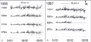
Fig. 8. Stick plots of the 3 hourly current measurements at mooring D in (a) 1996 and (b) 1997 at all measurement depths (see Fig. 1c) for April–September. Dates are mm/dd. Currents at 143m depth are directed predominantly northwards with a weak eastward component. the magnitude of the v-component (northward) takes an average value of 11.8 cms–1 (1996) and 12.4 cms–1 (1997) and that of the u-component (eastward) is 1.5 cms–1 (1996) and 4.0 cms–1 (1997).
Another difference between 1996 and 1997 becomes apparent if one checks which currents are observed on the day of the most pronounced positive salinity anomalies. It turns out that in 1996 (at about days 95, 130, 165, 205, 250 and 260) currents were weak and directed northward or were nearly zero at 143 m depth. In 1997 (at about days 105, 130, 145, 210, 225 and 250) currents were much more variable (with both southward and northward components) and also mostly stronger than in 1996. the lag correlation analysis between salinity anomalies and the u- and v-component of the ocean currents is not very conclusive for 1996 (Fig. 6b and d). This could indicate that the observed salinity anomalies were caused by local processes rather than by advection. In 1997 a positive (negative) salinity anomaly tends to be followed by currents with an eastward (westward) component 4–5 days later (see also section 4). This is difficult to interpret. the core region of the polynya and thus the region of the largest ice production is located west of the mooring position, in 1997 probably more often than in 1996 when the TNBP was on average larger than in 1997 (see Fig. 4). It is likely, therefore, that the main water-mass modification occurs west of the mooring position. the observed association of positive salinity anomalies with eastward currents a couple of days later could be the combined effect of salt enrichment of the water mass due to ice formation and of driving near-surface ocean currents by those winds which also opened and maintained the polynya. However, more work is needed to underline this. It could also be that the salinity anomalies observed in 1997 were purely driven by advection of water masses that were not modified in the TNBP before; this is likely for those salinity anomalies that are associated with currents with a westward component.
Following these results we suggest two explanations for the observed difference between 1996 and 1997. One explanation could be that the predominantly weak northward currents observed in 1996 in the context of positive salinity anomalies (see beginning of last paragraph) have created an environment that allows plumes of salt-enriched water emanated by the polynya to descend to the measurement depth without too much entrainment of fresher water masses from outside the polynya region. This environment could also have prohibited advection of the locally produced denser water masses out of TNB and thus out of the measurement site. In 1997, currents observed in the context of positive salinity anomalies (see beginning of last paragraph) were stronger and more variable. These currents might thus have caused an environment that was less suitable in which to observe a water-mass modification triggered by the polynya at the measurement depth of 143 m.
The second explanation is related to the fact that particularly the v-component of the currents was more variable in 1996 compared with 1997 at 143m depth, particularly before day 200. Actually, the currents switched direction between north- and southward several times. Although current speeds were smaller in 1996 than in 1997, this switch between directions could have allowed the advection of relatively warm and/or fresher water masses in the upper 100 m into the polynya area, modifying the local water mass and thus making plumes of high-salinity water emanated from the polynya become more visible because of the larger density contrast. the fact that ice production anomalies tend to be smaller in 1997 than in 1996 (see Fig. 5e and k) also aids in the explanation of why the effect of the polynya activity is more visible for 1996 compared with 1997.
The question as to whether the ice formation in the studied polynyas contributed substantially to HSSW or even AABW in the winters of 1996 and 1997 depends on various factors and cannot be answered here. Among these factors are the heat and salt content of the uppermost water layer at the end of summer, which are both known to be quite variable (e.g. Reference Budillon, Fusco and SpezieBudillon and others, 2000; Reference Fusco, Budillon and SpezieFusco and others, 2009). To these factors belongs the sea-ice cover at the end of summer, which can also be quite variable in extent and thickness depending on the atmospheric forcing during that summer and the preceding winter and thus on the ice growth and drift history (Reference Assmann and TimmermannAssmann and Timmermann, 2005; Reference Harangozo and ConnolleyHarangozo and Connolley, 2006). Finally, the normal pathways for surface currents and sea ice might be blocked by giant icebergs (e.g. Reference Brunt, Sergienko and MacAyealBrunt and others, 2006; Reference Martin, Drucker and KwokMartin and others, 2007). the sea-ice cover is influenced by, and in turn feeds back onto, the large-scale atmospheric circulation and is also influenced by the large-scale oceanic circulation (Reference Turner, Overland and WalshTurner and others, 2007; Reference Turner and OverlandTurner and Overland, 2009), in the case of the Ross Sea by the eastward-flowing coastal currents and waters from the branch of the Ross Gyre entering the shelf (Reference Jacobs, Giulivi and MeleJacobs and others, 2002). Furthermore, the mCDW influence is evident in the eastern Ross Sea, between 200 and 400 m depth, while in the western part of the basin its core is closer to the surface (i.e. shallower than 100 m) (Reference LocarniniLocarnini, 1994). the variability of these warm currents can be responsible for changes of sea ice and affecting surface processes including heat fluxes. Finally, properties of the western Ross Sea water masses are also influenced by the water masses leaving the caverns of the RIS. Depending on the properties of the entering water masses, the water masses leaving these caverns may carry the signal of enhanced ice-shelf bottom ablation and/or accretion of marine ice (e.g. Reference HellmerHellmer, 2004; Reference Robinson, Williams, Barrett and PyneRobinson and others, 2010). In years when these water masses carry an enhanced meltwater (ablation) signal, i.e. are fresher, it is likely that less sea ice would have to be formed inside the TNBP to modify the water masses.
6. Conclusions
We compared wintertime (April–September) area estimates of the TNBP based on satellite passive microwave data with in situ observations. Ocean salinity, temperature and currents from 1996 and 1997 are used from an instrument at 143 m depth in TNB. Polynya area anomalies and associated anomalies in ice production are significantly correlated to the observed salinity anomalies. Salinity anomalies lag area and/or ice-production anomalies by about 3 days in 1996. When moving a 90 day time window to carry out the lag correlation analysis up to 70% (about 30%) of the variability in the observed salinity can be explained by area and/or ice-production anomalies in the TNBP until the end of July (after July). This picture changes completely in 1997, when correlations are much smaller, less significant and occur at an apparent wrong time lag. the polynya area changed less often during 1996 than during 1997. Consequently, the TNBP was more persistent in 1996 than in 1997. the number of single polynya events, i.e. opening and closing of the TNBP, was larger in 1997 than in 1996, although this had no influence on the total ice production in both winters.
CTD casts from ship cruises into the TNB during summers 1994/95 to 1996/97 indicate a more pronounced layer of SSW in 1996 compared with 1995 and 1997. Observed currents at the mooring during periods of positive salinity anomalies indicate quite weak basically north- to northeastward directed currents in 1996 but stronger quite variable (southwestward and northeastward) currents in 1997. A lag correlation analysis shows evidence for a correlation between salinity anomalies and the u-component of the currents at the mooring in 1997. Based on our findings we suggest that the observed differences between 1996 and 1997 are the result of oceanic conditions that mimic the effect of plumes of salt-enriched water descending to the measurement depth, either because these are transported away too quickly and/or mix too quickly with fresher water entrained from outside the polynya area, or because shifting current directions cause the advection of water masses. These may (1) reduce the effect of the aforementioned plumes on the water masses at the measurement depth or (2) cause a salinity change that is similar to the one observed in association with polynya activity.
The mooring data as well as the polynya-area and ice-production data are just a subset of a time series spanning at least 10 years. the suggestion for future work is clearly to extend this analysis to a longer period to allow us to relate observed irregularities to anomalies in ice-shelf–sea-ice– atmosphere–ocean interaction in the Ross Sea region. One important addition to this study would be to include salinity and temperature measurements at greater depths. Another addition would be the inclusion of salinity observations from the ship cruises into the TNBP as carried out in the summers of 1995–97.
Acknowledgements
This work was supported by the German Science Foundation (DFG) under contracts Me 487/40-1, 40-2 and STA410/6-3, by CliSAP and by the CLIMA project of the PNRA. Helpful discussions with D. Flocco and the scientific editor, L. Smedsrud, and the comments of two anonymous reviewers are gratefully acknowledged.


