


Introduction
The ice streams that drain the West Antarctic ice sheet into the Ross Sea are separated by slowly moving inter-ice-stream ridges that rise 200–400 m above the level of the surrounding ice streams. Changes in the configuration of the ice streams would affect the flow and geometry of the ridges. Inter-ice-stream ridges therefore contain a record of past ice-stream activity in their geometry and internal stratigraphy.
Ice-penetrating radar and global positioning system (GPS) survey measurements made on three inter-ice-stream ridges in West Antarctica, namely, Siple Dome (82° S, 148° W), ridge DE (80.5° S, 140° W) and ridge BC (83° S, 140° W), reveal the present geometry of the surface and internal stratigraphy (Fig. 1). We use these data to infer the stability of the divide position and the pattern and history of the spatial accumulation distribution across the ridges. The history of the divide position may indicate relative thickening or thinning of the ice streams bounding an inter-ice-stream ridge. The three ridges considered together give some information about the large-scale pattern of thickness change in the ice-stream system across the Siple Coast.
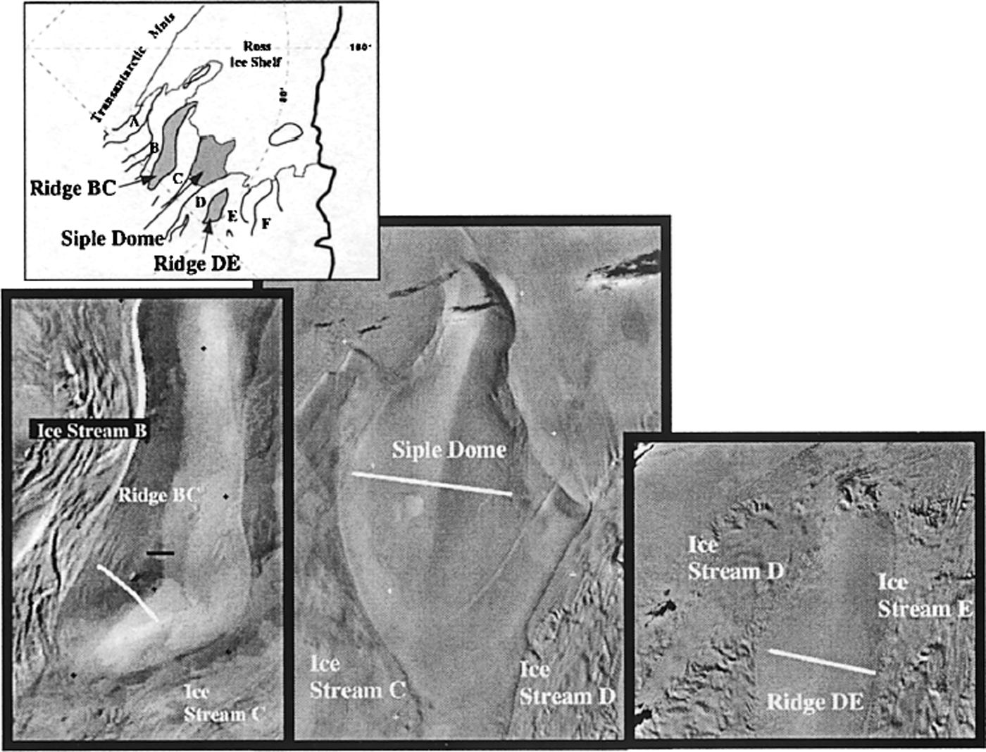
Fig. 1. Satellite images of three inter-ice-stream ridges in West Antarctica: ridge DE (Landsat), Siple Dome Advanced Very High Resolution Radiometer (AVHRR) and ridge BC (AVHRR) (Reference Scambos, Kvaran and FahnestockScambos and others, 1999; personal communication from P. Vornberger, 1998). White linesshow location of radio-echo sounding (RES) measurements in Figure 2.
Measurements and Data Analysis
Surface-based radar and GPS survey measurements were made across Siple Dome during the 1994 and 1996 field seasons as part of a collaborative project among the University of Washington, St Olaf College and the University of Colorado (Reference Raymond, Nereson, Gades, Conway, Jacobel and ScambosRaymond and others, 1995; Reference Scambos and NeresonScambos and Nereson, 1995; Reference Jacobel, Scambos, Nereson and RaymondJacobel and others, 2000). We made radar and GPS survey measurements across ridges DE and BC during the 1998/99 field season. The low-frequency (2–3 MHz) radar system and the basic data-analysis techniques used for all three field sites have been described elsewhere (Reference Jacobel, Scambos, Raymond and GadesJacobel and others, 1996; Reference Nereson, Raymond, Waddington and JacobelNereson and others, 1998a; Reference Gades, Raymond, Conway and JacobelGades and others, 2000). Measurements were usually made every 20 m, but sometimes every 100 m. Signal travel time is converted to depth using a ray-tracing program (e.g. Reference WeertmanWeertman, 1993) that assumes an ice-density profile based on measurements from a Siple Dome ice core (Reference Mayewski, Twickler and WhitlowMayewski and others, 1995).
The surface elevation S(x) along each profile line was surveyed with dual-frequency Trimble 4000 GPS receivers in continuous kinematic mode (uncertainty relative to the base station ∼0.1 m). Poles positioned every 5 km along the profile lines were surveyed with differential static methods. Ice thickness H(x), determined from radar measurements, is subtracted from the surface profile S(x) to obtain the bedrock topography R(x) at each site. Figure 2 shows the radar profiles, corrected for surface elevation, for each of the ridges.
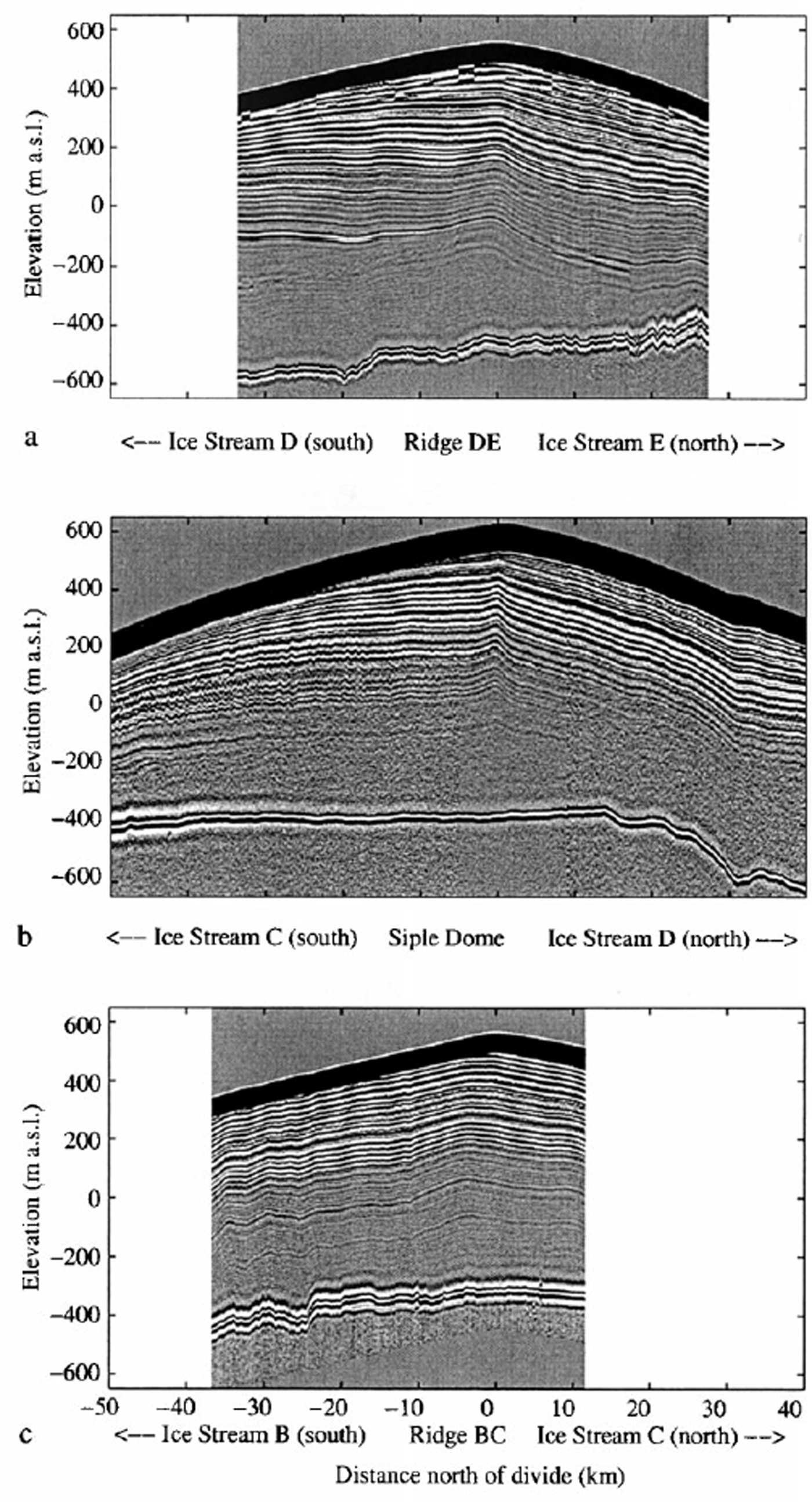
Fig. 2. RES profiles collected along the white lines in Figure 1 for ridge DE (a), Siple Dome (b) and ridge BC (c). Surface topography determined from GPS surveys.
For all ridges, the ice is about 1000 m thick and overlies a relatively flat bed. Internal layers are visible in all profiles to at least 70% depth. The internal layers likely arise from variations in the electrical properties of the deposited snow (Reference HarrisonHarrison, 1973; Reference Paren and RobinParen and Robin, 1975; Reference HammerHammer, 1980; Reference Moore, Wolff, Clausen and HammerMoore and others, 1992). We assume that they represent isochrones (or horizons of constant age since deposition on the upper surface).
The vertical location of a given internal layer is defined by selecting the two-way travel time of the maximum or minimum reflection voltage in a prescribed time window selected to bracket the layer. Each layer is smoothed in the horizontal domain with a low-pass filter (cut-off wavenumber = 1/1000 m−1). The uncertainty associated with identifying an internal layer depends on the wavelength used, the roughness of the internal layer and its depth (Reference Nereson, Raymond, Waddington and JacobelNereson and others, 1998a, Reference Nereson, Raymond, Jacobel and Waddington2000). The error ranges from 5 to10 m for frequencies of 2–3 MHz, depending on layer depth. The uncertainty in the ice thickness is usually less (about 6 m), because the reflected signal from the bed is stronger, sharper and unambiguous.
Qualitative Description of Data
A prominent feature of the internal layer shapes for Siple Dome and ridge DE is an up-warp beneath the ice divide (Fig. 2). This feature is expected beneath stable ice divides (Reference RaymondRaymond, 1983; Reference HvidbergHvidberg, 1996) due to the strain-rate softening in Glen’s non-linear ice-flow law (Reference PatersonPaterson, 1994, p. 85). The up-warp feature can also be caused by a local accumulation low over the ice divide, perhaps due to wind-scouring (Reference Fisher, Koerner, Paterson, Dansgaard, Gundestrup and ReehFisher and others, 1983; Reference Vaughan, Corr, Doake and WaddingtonVaughan and others, 1999). In either case, the shape and amplitude of this feature is affected by the history of the divide position.
Qualitatively, the divide feature differs markedly among the ridges. At Siple Dome, the feature is most pronounced (largest warp amplitude) and confined to within about two ice thicknesses of the divide (Fig. 2b). At ridge DE, it is less pronounced in amplitude and is spread over a wider zone extending to about four ice thicknesses of the divide (Fig. 2a). For ridge BC, the feature is non-existent beneath the present divide, but there is a broad up-warp feature about 5 km south of the present divide that appears to be unrelated to surface or bed topography (Fig. 2c). For both Siple Dome and ridge DE, the feature is not vertically aligned, but tilted so that the apex of deep layers lies to the south (left in Fig. 2) of the present divide. We interpret this tilt as evidence for migration of the ice divide and use an ice-flow model to quantify the rate of divide migration. The absence of any detectable up-warp on ridge BC suggests that the divide position there is highly non-steady.
The spatial distribution of accumulation across the inter-ice-stream ridges can also be inferred from the shape of the internal layers. Figure 2 shows that for all the inter-ice-stream ridges a given internal layer is found at shallower depths on the southern flank than on the northern flank. This suggests an accumulation gradient across the ridges, with more snow deposited on the northern flanks. This is consistent with the hypothesis that the moisture flux into this area of West Antarctica comes from storms that originate in the Amundsen Sea and travel southward and westward over the ice-stream area, depositing more snow on the windward sides of the ridges from orographic lifting (Reference BromwichBromwich, 1988; Reference Carrasco and BromwichCarrasco and Bromwich, 1994; Reference HoganHogan, 1997). We use a kinematic ice-flow model to quantify the spatial pattern of accumulation relative to the accumulation rate at the summit of each ridge and to determine possible changes in the spatial pattern over time.
History of Divide Positions
Model parameterization
We use the kinematic model described in Reference Nereson, Raymond, Waddington and JacobelNereson and others (1998a) to quantify the rate of divide migration. We assume the up-warped internal layers beneath all the divides arise solely from the non-linearity of Glen’s ice-flow law and not accumulation scouring at the divide. Although up-warped internal layers can also be caused by a local minimum in the accumulation pattern, Reference Nereson, Raymond, Waddington and JacobelNereson and others (1998a) showed that the inferred divide migration rate does not depend strongly on what mechanism for layer up-warp formation is assumed. In addition, strain patterns consistent with non-linear ice flow have been measured at Siple Dome (Reference PettitPettit and others, 1999).
The magnitude of the velocity field is determined solely from mass-balance requirements. Its depth distribution is prescribed according to a partitioning between flank and divide flow, and these are determined from an independent stress-balance model of ice flow assuming Glen’s flow law with n = 3. We assume that ice thickness H is uniform in the vicinity of the divide and that the accumulation pattern b(x) is constant in time. Divide migration is simulated by shifting the velocity field at a constant rate during the calculation of ice flow. The migrating-divide situation is steady-state so that the pattern of the velocity field relative to the migrating divide is time-independent. With these assumptions, the velocity field can be written as


where
![]() is a non-dimensional vertical coordinate,
is a non-dimensional vertical coordinate,
![]() , ξ(x, z) is the shape of the variation in horizontal velocity with depth, and
, ξ(x, z) is the shape of the variation in horizontal velocity with depth, and
![]() (Reference Nereson, Raymond, Waddington and JacobelNereson and others, 1998a). The velocity shape function ξ(x, z) is a linear combination of a shape function typical of near-divide flow
(Reference Nereson, Raymond, Waddington and JacobelNereson and others, 1998a). The velocity shape function ξ(x, z) is a linear combination of a shape function typical of near-divide flow
![]() and a shape function typical of flank flow
and a shape function typical of flank flow
![]() ,
,
where 0 ≤ φ(x) ≤ 1 describes the partitioning between flank-and divide-flow regimes. Following Reference Nereson, Raymond, Waddington and JacobelNereson and others (1998a), we allow a hinge-like accumulation pattern b(x) with two gradient parameters G s and G n that describe the accumulation gradient on the south (x < 0) and north (x > 0) sides of the divide, respectively.
To simulate divide migration, the flow field is moved at a rate m in the same reference frame as the divide, so that x = 0 is always the divide position, and the horizontal velocity in the divide reference frame is
where M = m/b(0) is a constant divide-migration rate m scaled to a reference accumulation rate b(0). The expression for vertical velocity
![]() is unchanged.
is unchanged.
Velocity equations (1), (2) and (4) with shape functions given by Equations (3) and (5), and the parameters M, G n and G s define the kinematic model for isochrone deformation due to a non-linear flow law. Tracking the motion of ice particles in this flow field through time predicts the shape of isochrone horizons. Three non-dimensional free parameters, M, G s and G n, are varied to find the combination that best fits the observed layer shapes. A mismatch index, defined in Reference Nereson, Raymond, Waddington and JacobelNereson and others (1998a, equation (15)), is used to compare the observed to the calculated layer shapes in a way that accounts for errors in the model and in the data. A mismatch index less than 1 indicates that the calculated layer shapes match the observed layer shapes to within one standard deviation defined by errors in the model and the data.
Siple Dome
For Siple Dome, the shape functions ζf and ζdiv are given by an eighth-order Chebyshev polynomial fit to a steady-state, finite-element calculation of the flow field at x = 10 km and x = 0 km, respectively (Reference Nereson, Waddington, Raymond and JacobsonNereson and others, 1996). The finite-element model assumes Glen’s flow law to describe non-linear ice flow with the degree of non-linearity described by n = 3. The partitioning function φ(x) is given by the continuously differentiable, even function:

where ℓ 1 = 775 m and ℓ 2 = 3740 m. The characteristic accumulation rate is taken to be b(0) = 0.10 m a−1 (Reference KreutzKreutz and others, 1999).
As discussed in Reference Nereson, Raymond, Waddington and JacobelNereson and others (1998a), the predicted divide-migration rate is 0.20–0.50 m a−1 with a mean value of about 0.30 m a−1, assuming that the warp feature is caused solely by non-linear ice flow. The depth distribution of residuals shows no compelling reason to invoke non-steady motion of the ice divide. Based on the present vertical strain and the amplitude of the divide feature in the layers, Reference Nereson, Raymond, Waddington and JacobelNereson and others (1998a) estimate that the Siple Dome divide has been migrating northward for at least a few thousand years.
Ridge DE
The wide zone of up-warped layers beneath the ridge DE divide is unrelated to bed topography and is present in two parallel profiles across the divide, spaced 8 km apart. The trend of the up-warp apex is tilted to the north, indicating possible divide migration. We use the same ice-flow model and layer-shape analysis as used for the Siple Dome layers to quantify the rate of divide migration. We set b(0) = 0.10 m a−1 (Reference Thomas, MacAyeal, Eilers, Gaylord, Hayes and BentleyThomas and others, 1984; Reference Bindschadler, Vornberger, Blankenship, Scambos and JacobelBindschadler and others, 1996; Reference Venteris and WhillansVenteris and Whillans, 1998) and use the partitioning function given by Equation (5) to calculate internal layer shapes for various combinations of the parameters G n, G s and M. The calculated layers are compared to the observed layers of ridge DE using a mismatch index that accounts for errors in the model and the data (Reference Nereson, Raymond, Waddington and JacobelNereson and others, 1998a, equation (15)).
No combination of the three parameters produces a good match to the observed layer shapes. The spatial pattern of residuals indicates that a good match is not possible because the observed divide zone in the ridge DE layers is about twice as wide as the model divide zone. At low migration rates M, the modeled up-warp is narrower than the observed up-warp; and at high M, the modeled up-warp is wide because of divide motion, but the amplitude is much lower than is observed. One possible explanation is that the large width of the observed divide zone is caused by rapid fluctuations in divide position about a mean position, and the tilt of the up-warp axis results from migration of the mean divide position. Evidence to support this hypothesis is that the present topographic divide is offset 700 m southward from the peak of the shallowest layer, and 1000 m southward from the upward extension of the trend of the apex axis to the ice surface. In addition, the ridge DE divide is rounder than Siple Dome. Slopes at one ice thickness from the divide are about 50% less at ridge DE than at Siple Dome, where the divide zone is narrow and consistent with theoretical estimates of its width (Fig. 3) (Reference RaymondRaymond, 1983).

Fig. 3. Smoothed surface slopes for the three inter-ice-stream ridges: Siple Dome (thick solid line) ridge DE (dashed line) and ridge BC (thin solid line).
Rapid fluctuation of the ice divide could be caused by rapid changes in the large-scale accumulation pattern (Reference HindmarshHindmarsh, 1996), or asymmetric changes in elevation of the bounding ice streams (Reference Nereson, Hindmarsh and RaymondNereson and others, 1998b). One simple representation of a rapidly fluctuating divide position is x div = A sin (ωt). The amplitude of the fluctuation A must be sufficiently small that a divide spends most of its time within one ice thickness of its mean position and an up-warp feature is allowed to develop in the internal layers. Therefore, we assume A ≤ H.
The frequency of the fluctuation ω must be sufficiently fast (≫ b/H ≈ 10−3 a−1) that the fluctuation serves only to broaden the divide zone and does not produce its own signature in the internal layer pattern. Upper limits on ω are associated with the dynamic response of the divide position. Changes in the large-scale accumulation pattern that are too fast will not cause the divide position to fluctuate since the geometry of the ice sheet will not have enough time to respond to the accumulation pattern. The response time of the divide position to stochastic perturbations in the accumulation pattern is about 102 years (Reference HindmarshHindmarsh, 1996; Reference Nereson, Hindmarsh and RaymondNereson and others, 1998b). The response time can be longer if the divide fluctuation is caused by changing elevation of the bounding ice streams since it takes additional time for the effect to appear at the ice divide. We therefore assume 10−3 a−1 < ω < 10−2 a−1.
Substitution of x − x div = x − A sin (ωt) for x in Equation (5) and numerical integration over time yields an effective partitioning function representing the divide zone for the mean divide position. Figure 4 shows this effective partitioning function for various values of A. For A < ℓ 1, the divide zone includes a single maximum. For A > ℓ 1, the divide zone is wide and develops two maxima at the ends of the zone. This feature is a result of the assumed sinusoidal fluctuation of the divide that causes the divide to spend more time at the extreme ends of the fluctuating zone. The amplitude of the partitioning function decreases with increasing A, reflecting the greater amount of time the ice experiences flank flow in the zone of fluctuation. The time average conserves the area under the curve.

Fig. 4. Divide-/flank-flow partitioning function for a sinusoidally fluctuating divide obtained from numerical integration of φ(x − A sin ωt) over time (solid lines) and approximated using Equation (6) (dashed lines) for fluctuation amplitude values A/ℓ 1 = 0, 0.5, 1, 2, 3 and 5.
In our model, we use an analytical approximation to this time-averaged numerical solution that is continuously differentiable over our domain and reduces to Equation (5) when A = 0:

where Φ is the maximum value of the effective partitioning function determined by numerical integration of the sinusoid fluctuation. Figure 4 shows the approximating function. The function provides a reasonable representation for 0 ≤ A/ℓ 1 ≤ 5. The curve connecting the apex of each internal layer intersects the surface 1000 m from the topographic divide. Since the ice thickness is about 1000 m, this offset is at the upper limit of possible values for A. We therefore assume that the present divide is near an extreme excursion from its mean position and A = 1000 (A/ℓ 1 = 1.3). Also, we shift the domain 1000 m northward so that the present mean divide position is in line with the trend of the axis connecting the apex of the shallowest layers. With this new partitioning function, the effective divide zone is about twice as wide as the stationary divide zone. Using the new partitioning function (6) in Equation (3) and the velocity field described by Equations (1), (2) and (4), we calculate new sets of isochrones and perform the minimization to find the best-fitting combination of parameters.
The results show that again no combination of parameters produces a fit to all the observed layers to within the measurement error. The mismatch is largest for the two deepest layers, which have a large bump amplitude compared to the model and are offset southward of the present divide by 2 km. Under a constant divide migration, a divide bump is not expected to exist outside of the divide zone (Nereson and Waddington, in press). The pronounced bump outside of the divide zone suggests divide migration at a non-constant rate. We hypothesize that the ridge DE divide was once located a few kilometers south of its present position for a sufficiently long time (∼ τ) that a divide bump was allowed to develop at depth. Since the divide moved from this location, the deep layers have retained some of their shape from the old flow regime.
Restricting our analysis to all but the deepest two layers with the anomalously large warp, we find the model parameters G n = 0.3 ± 0.1, G s = 0.1 ± 0.1, M = 5 ± 1 produce calculated layer shapes that fit the observed layer shapes to within the expected errors (Fig. 5). This implies northward migration of the mean position of the ridge DE divide at Mb(0) = 0.4–0.6 m a−1. If we assume that the old divide position was located over the up-warp of the deepest layers, about 2 km south of the present mean divide position, then the mean divide position has been migrating northward for at least 3 kyr.

Fig. 5. (a) Observed internal layer shapes at ridge DE from RES data (black), and calculated internal layer shapes from model with fluctuating divide, no divide migration and uniform accumulation distribution (gray), (b) Observed (black) and calculated (gray) internal layer shapes. Calculated layer shapes correspond to parameters G n = 0.04, G s = 0.00, M = 5 that produce the minimum mismatch index. The two deepest layers shown were excluded from the mismatch calculation.
Ridge BC
The internal layers beneath the ridge BC divide show no evidence of up-warping, indicating that the divide position has not been within a few ice thicknesses of its present position for several thousand years. However, 5 km south of the present divide, toward Ice Stream B2, there is a broad up-warp feature that is unrelated to bed or surface topography (Figs 2 and 6). We interpret this feature as the remnant of an up-warp that developed when the divide formerly occupied this site. We hypothesize that the ice divide was 5 km south of its present position for a sufficiently long period to form a divide feature and has moved to its present position quickly and recently so that the old divide feature in the internal layers is still intact and a new divide feature has not yet formed.

Fig. 6. Observed internal layer shapes from RES data for ridge BC. Up-warp feature in the internal layer pattern is offset from the present divide position by 5 km.
To quantify this hypothesis and place limits on how quickly and how recently the divide has moved, we use a simple analytic model of divide-bump formation conceived by Reference Waddington, Conway, Gades, Nereson and ClowWaddington and others (1998). Suppose ice beneath a steady-state divide (subscript d) deforms according to a quadratic vertical velocity pattern (Reference RaymondRaymond, 1983), and ice on the flanks (subscript f) according to a linear vertical velocity pattern (Reference NyeNye, 1963):
where
![]() is the scaled height above the bed, and t denotes time before present, or age of the ice, in units of H/b = τ. Now consider an ice sheet with a moving divide so that there is a site c that experiences first flank then divide (or first divide then flank) flow. The vertical velocity at this site can be expressed as a linear combination of flank and divide flow,
is the scaled height above the bed, and t denotes time before present, or age of the ice, in units of H/b = τ. Now consider an ice sheet with a moving divide so that there is a site c that experiences first flank then divide (or first divide then flank) flow. The vertical velocity at this site can be expressed as a linear combination of flank and divide flow,
where 0 ≤ a(t) ≤ 1. Equation (8) can be solved analytically for
![]() for some special cases of a(t). We define a divide bump at various stages of its formation and decay as the height difference of a layer at the site that experiences a combination of flank and divide flow (subscript c) relative to a site that experiences only flank flow (subscript f):
for some special cases of a(t). We define a divide bump at various stages of its formation and decay as the height difference of a layer at the site that experiences a combination of flank and divide flow (subscript c) relative to a site that experiences only flank flow (subscript f):
Consider two cases: (1) the divide is at site c for a long time and then moves quickly away at time t = t* before present; (2) site c experiences first flank flow for a long time, then the divide quickly moves onto site c at time t = t* before present. For case (1), site c experiences first divide flow for times (ages) t ≥ t* before present, then flank flow for times (ages) t ≤ t* so that a(t) = 1 for t > t* and a(t) = 0 otherwise. After integration over time of
![]() and
and
![]() , Equation (9) yields
, Equation (9) yields

Substitution of the age–depth relation
![]() in Equation (10) gives the distribution of bump amplitude with depth. Figure 7 shows how the divide bump varies with depth for various abandonment times t*. For t* = 0.5, the bump feature is reduced to about half of its initial amplitude at depth and is not detectable in the upper half of the ice sheet where the ice has experienced only flank-flow deformation since abandonment of the divide position.
in Equation (10) gives the distribution of bump amplitude with depth. Figure 7 shows how the divide bump varies with depth for various abandonment times t*. For t* = 0.5, the bump feature is reduced to about half of its initial amplitude at depth and is not detectable in the upper half of the ice sheet where the ice has experienced only flank-flow deformation since abandonment of the divide position.

Fig. 7. Divide-bump size
![]() at depths
at depths
![]() at a former steady divide site for various times t* since the divide moved away, t* = 0, 0.1, 0.3, 0.5, 1, 2 in units of τ = H/b ≈ 104 years for ridge BC. Dotted line marks where
at a former steady divide site for various times t* since the divide moved away, t* = 0, 0.1, 0.3, 0.5, 1, 2 in units of τ = H/b ≈ 104 years for ridge BC. Dotted line marks where
![]() .
.
In the second case, site c experiences first flank flow for times (ages) t ≥ t* before present, then divide flow for times (ages) t ≤ t* so that a(t) = 0 for t > t* and a(t) = 1 otherwise. The divide bump is given by

Figure 8 shows the divide bump that develops in the ice column (using the age-depth substitution
![]() after the divide moves onto a new site at various times t*. The largest divide bump occurs at depths corresponding to t = t*, so the bump develops most at shallow depths when the divide first moves on to the new site. After t = 1, the maximum bump size occurs deep in the ice column.
after the divide moves onto a new site at various times t*. The largest divide bump occurs at depths corresponding to t = t*, so the bump develops most at shallow depths when the divide first moves on to the new site. After t = 1, the maximum bump size occurs deep in the ice column.

Fig. 8. Divide-bump size
![]() at depths
at depths
![]() at a former flank site for various times t* since the divide moved onto the site, t* = 0.1, 0.2, 0.3, 0.5, 1, 2, 20 in units of τ = H/b(0) ≈ 104 years for ridge BC. Dotted line marks where
at a former flank site for various times t* since the divide moved onto the site, t* = 0.1, 0.2, 0.3, 0.5, 1, 2, 20 in units of τ = H/b(0) ≈ 104 years for ridge BC. Dotted line marks where
![]() .
.
These results can be used to place limits on the motion of the ridge BC ice divide. Although the velocities in Equation (7) are extreme representations that exaggerate the difference in flow between divide and flank sites, the simplicity of the solution is useful for making order-of-magnitude estimates of divide-bump growth and decay. An anomalous bump with an amplitude of nearly 10 m
![]() is detectable in the internal layers of ridge BC at the hypothesized old divide site (5 km south of the present divide) as shallow as 20% of the ice thickness. Figure 7 shows that a bump of that amplitude would exist at such shallow depths only if the divide moved away within the last 0.1 τ years, or 0.1 H/b ≈ 1000 years (assuming b ≈ 0.10 m a−1 (Reference Venteris and WhillansVenteris and Whillans, 1998) and H ≈ 1000 m). In addition, any remnant divide feature in a flank-flow regime would be advected downslope. An estimate of horizontal velocity from a simple continuity argument
is detectable in the internal layers of ridge BC at the hypothesized old divide site (5 km south of the present divide) as shallow as 20% of the ice thickness. Figure 7 shows that a bump of that amplitude would exist at such shallow depths only if the divide moved away within the last 0.1 τ years, or 0.1 H/b ≈ 1000 years (assuming b ≈ 0.10 m a−1 (Reference Venteris and WhillansVenteris and Whillans, 1998) and H ≈ 1000 m). In addition, any remnant divide feature in a flank-flow regime would be advected downslope. An estimate of horizontal velocity from a simple continuity argument
![]() gives
gives
![]() . After 1000 years, features near the surface should be displaced downslope from features at depth by about 500 m. However, the remnant bump feature at ridge BC is vertically aligned and shows no sign of such downslope advection, suggesting that the divide moved from this old site much less than 103 years ago.
. After 1000 years, features near the surface should be displaced downslope from features at depth by about 500 m. However, the remnant bump feature at ridge BC is vertically aligned and shows no sign of such downslope advection, suggesting that the divide moved from this old site much less than 103 years ago.
Figure 8 shows that if the divide has been at its present location for >0.15τ, a bump larger than 10 m should have formed at a depth of 0.2 H. We do not see such a feature in the internal layers, and conclude that the divide has been at its present position for <1.5 kyr. If the broad up-warp in the internal layers 5 km south of the present divide position is a remnant marker of a former divide position, then our analysis suggests that the divide moved off that position within the last 103 years or less. If the divide moved steadily northward to its present position in that time, then the migration rate is at least 5 m a−1.
However, it is possible that the up-warp is not an old divide signature. These data were collected at the rounded upstream end of ridge BC east of the summit (Fig. 1) where there may be a component of flow perpendicular to the profile line. The up-warp in the layering could be caused by bedrock features outside the plane of the profile. Although other radar profiles collected during the same field season show a flat bed, there is a single anomalous bedrock high associated with the dark spot in the satellite image to the west of the main profile (Fig. 1). This bedrock feature is several ice thicknesses from, and not in line with, the up-warp in the internal layering, but we cannot completely rule out its possible influence on the layers observed in the main profile.
Another radar profile obtained across the ridge BC divide about 10 km westward of the summit spanned about 7 km on either side of the divide (black line in Fig. 1). This profile shows no sign of a divide up-warp feature in the internal layers, suggesting that the divide at this location on ridge BC has also recently arrived at its present position. There is no sign of an anomalous up-warp feature elsewhere in the 14 km profile, suggesting that the divide has not occupied a site within 7 km of its present position for a sufficient amount of time to form a divide feature in the internal layers.
Discussion
Of the three inter-ice-stream ridges, the divide position at Siple Dome appears most stationary because of its well-developed, narrow up-warp in the internal layers. Previous analysis suggests that the divide has been migrating northward at a steady rate of about 0.2–0.5 m a−1 for the past few thousand years. The divide position at ridge DE is more variable than at Siple Dome, but its mean position is sufficiently stationary that a divide feature exists beneath the present ice divide. The up-warp in the internal layer pattern is wider than theory predicts, and we suggest this is a result of fluctuations of the divide position around a relatively stable mean position that has been migrating northward toward Ice Stream E at about 0.4–0.6 m a−1. Ridge BC has the most variable divide position of all the ridges, with no distinct feature in the internal layer pattern beneath the present ice divide at two locations (separated about 30 km) along the divide. A broad up-warp in the internal layer pattern 5 km south of the present divide suggests that is a recent location of the ice divide. If so, a simple analytic calculation suggests that the divide has moved off this old location within the last 1000 years, migrating to its present position at a minimum mean rate of 5 m a−1.
In all cases the direction of divide motion is northward. Possible causes of divide migration include changing elevation of the ice-stream boundaries and/or a changing spatial distribution of accumulation. We can use the radar internal layer data to examine possible changes in the spatial accumulation pattern over time.
Spatial accumulation patterns
Model parameterization
Reference Nereson, Raymond, Jacobel and WaddingtonNereson and others (2000) used a kinematic ice-flow model to quantify the long-term average accumulation pattern at Siple Dome. Here we apply the same model to ridges DE and BC to determine the spatial distribution of accumulation and possible past changes in this distribution. Following Reference Nereson, Raymond, Jacobel and WaddingtonNereson and others (2000) the magnitude of the velocity field is determined solely from mass-balance and continuity requirements. We allow ice thickness H(x) to vary with position x because we are interested in the geometry of the layers along the entire ridge, not just near the divide. The steady-state accumulation pattern b(x) across the ridge is inferred from the shape of the internal layers far away from the divide zone. Therefore, the divide zone is neglected; the shape of the velocity variation with depth does not vary with position, and is represented by a flank shape function:
The velocity equations are simplified by performing the calculation of particle paths on a regular grid using the normalized vertical coordinate
![]() , where R(x) is bedrock elevation (Reference ReehReeh, 1988). The velocity of an ice particle in the regular grid is
, where R(x) is bedrock elevation (Reference ReehReeh, 1988). The velocity of an ice particle in the regular grid is


Equations (13) and (14) describe a continuous flow field for ice particles given ice thickness H(x), bedrock geometry R(x), shape function
![]() and accumulation pattern b(x).
and accumulation pattern b(x).
Following Reference Nereson, Raymond, Jacobel and WaddingtonNereson and others (2000), the accumulation pattern b(x) is represented by an arctangent function,

where b(0) is the accumulation rate at the divide in ice-equivalent units and ⋆, which can be either s or n, denotes values for the south and north sides of the divide. Different scale lengths λ ⋆ and amplitudes α ⋆ for the south (s) and north (n) sides of the divide can accommodate a wide range of accumulation patterns. We set b(0) = 0.10 m a−1 for all ridges (Reference Bindschadler, Vornberger, Blankenship, Scambos and JacobelBindschadler and others, 1996; Reference Venteris and WhillansVenteris and Whillans, 1998; Reference KreutzKreutz and others, 1999). However, b(0) merely scales the flow field; it affects neither the spatial pattern of the flow field nor the corresponding isochrone shapes.
Ice particles originating at the surface are tracked through time according to the velocity field (Equations (13) and (14)) driven by the accumulation pattern (Equation (15)). The resulting age field is contoured to obtain the internal layer pattern. The parameters, α s, α n , λ s and λ n, are varied in order to find the combination that produces the best match to the observed layer shapes. Calculated and observed layers are compared using a mismatch index for south and north sides of the divide, respectively (Reference Nereson, Raymond, Jacobel and WaddingtonNereson and others, 2000, equation (13)). We do not attempt to match layers within 2–4 ice thicknesses of the divide since this is a zone of special flow that is not taken into account by the model.
Results
Reference Nereson, Raymond, Jacobel and WaddingtonNereson and others (2000) showed that all the internal layers at Siple Dome can be matched using a steady-state accumulation pattern with parameters α n = 0.2, λ n = 5 km, α s = 0.8 and λ s = 50 km. Figure 9 shows the range of accumulation patterns that produce calculated internal layer shapes within one standard deviation of the measured shapes (black range). The depth distribution of their residuals showed that the accumulation rates north of the divide could have decreased over time.

Fig. 9. Range of accumulation patterns that fit the data to one standard deviation. All accumulation patterns are determined relative to the accumulation rate at the divide.
For ridge DE, no combination of parameters produces calculated layer shapes that match the observed layer shapes to within the errors. The mismatch is especially large for ridge DE layers south of the divide. Figure 10 shows the depth distribution of residuals for a range of accumulation gradient strengths (α n and α s). Deeper (older) layers are fit best with a larger value of α n, while shallow layers are fit best with a lower value. This suggests a possible change in the accumulation pattern at ridge DE over time such that more accumulation was deposited north of the divide in the past. If so, the strength of the south–north accumulation gradient has decreased over time.

Fig. 10. Ridge DE mismatch pattern. The shaded area shows how the mismatch between the modeled and observed layers varies with average depth (or age) of the layer for various values of α n or α s ; these parameters indicate the accumulation gradient strength (see Equation (15)) on the north (right panel) and south (left panel) sides of the divide. The transition lengths λ s and λ n are fixed at 30 and 3 km, respectively.
We now focus on the recent accumulation pattern, and restrict the analysis at ridge DE to the shallowest eight layers in the upper half of the ice column representing the past several thousand years. Figure 9 shows the range of accumulation patterns that produce a fit to the data to within one standard deviation (hatched region). The parameters α n = 0, λ n = 0–5 km, α s = 0.6 and λ s = 20 km produce the best match. As at Siple Dome, the analysis suggests a strong south–north accumulation gradient over ridge DE. It is nearly uniform south of the divide. It is large on the north side close to the divide but decreases to a small value beyond a few ice thicknesses from the divide.
Since we believe that the shape of the internal layers 3–8 km south of the ridge BC divide is due to a remnant divide-flow regime, we omit this section from the accumulation pattern analysis. In addition, our data cover only a small portion of the northern flank, so we do not calculate separate mismatch indices for northern and southern sides of the divide. Instead we calculate a single mismatch index for a single set of accumulation parameters α and λ that are applied on both sides of the divide. Figure 9 shows the range of accumulation patterns that fit the data to one standard deviation for all ridge BC layers (shaded region). The depth distribution of residuals shows no evidence for changes in the pattern over time. However, for ridge DE and Siple Dome, the evidence for changes in the accumulation pattern was strongest in the layers on the northern flank; the ridge BC data cover only a small region of the northern flank. The results suggest a south–north accumulation gradient, though this is not as strong as at Siple Dome or ridge DE.
Discussion
On all three ridges we find lower accumulation rates on the southern flank, and higher accumulation rates on the northern flank (relative to accumulation rate at the divide). The gradient is strongest for ridge DE, which is closest to the Amundsen Sea, and weakest for ridge BC, which is farthest inland. The dominant moisture source for the Siple Coast is believed to be storm systems that originate near the Amundsen Sea low, then travel southwestward over West Antarctica (Reference BromwichBromwich, 1988; Reference Carrasco and BromwichCarrasco and Bromwich, 1994; Reference HoganHogan, 1997). The general accumulation gradient across the inter-ice-stream ridges is consistent with these moisture tracks and suggests that southward-traveling weather systems deposit more snow on the northern flanks of the ridges from orographic uplift. The weakening of the accumulation gradient with distance from the Amundsen Sea is consistent with the hypothesis that storms from the Amundsen Sea area first travel south, perpendicular to ridge DE and Siple Dome, and then turn westward toward the Ross Sea, tracking along ridge BC. This change in storm direction, from perpendicular to the ridges to along the ridges, may decrease the orographic lifting and its associated pattern of accumulation distribution.
Past Elevation of Ice Streams
The internal layer pattern in the vicinity of the ice divides and over large cross-sections of three inter-ice-stream ridges is influenced by past activity of the ice streams that bound them. We find evidence for northward divide migration at Siple Dome and ridge DE, and possibly also at ridge BC. Possible causes of divide migration include changes in the spatial distribution of accumulation and changes in elevation and margin position of the ice streams at the boundaries of the ridges. Our analysis of the accumulation pattern determined from the large-scale internal layers shows that a decrease in the south-to-north accumulation gradient over time for Siple Dome and ridge DE is possible. Reference Nereson, Hindmarsh and RaymondNereson and others (1998b) showed that a reduction in the south-north accumulation gradient would tend to cause southward (not northward) divide migration. Therefore, we are motivated to discount changes in the spatial accumulation gradient as the cause of the northward divide migration; instead we invoke changes in the bounding ice streams.
If the divide migration is caused solely by changing elevation at the boundaries of the ridges, then we can place limits on the relative elevation history of the Siple Coast ice streams. Reference Nereson, Hindmarsh and RaymondNereson and others (1998b) used a linearized perturbation analysis of steady-state flow to determine the time-dependent divide position for a given elevation history of the bounding ice streams.
They estimated that Siple Dome divide migration of about 0.3 ± 0.1 m a−1 requires thinning of Ice Stream C (relative to D) at 0.025 ± 0.010 m a−1. Since it takes time for the effects of changes at the boundaries to affect the divide, the divide position at Siple Dome has not yet responded to the shut-down and subsequent thickening of Ice Stream C about 140 years ago (Reference Retzlaff and BentleyRetzlaff and Bentley, 1993). Based on the elevation of relict ice-stream margins bounding Siple Dome, Reference NeresonNereson (2000) showed that the divide migration is likely caused by thinning of the Ice Stream C trunk prior to its shut-down, rather than by thickening of Ice Stream D.
Our analysis suggests that the ridge DE divide has been migrating toward Ice Stream E at (5 ± 1) b(0) ≈ 0.5 ± 0.1 m a−1 for a few thousand years. A perturbation analysis similar to that for Siple Dome shows that this migration rate requires the upper part of Ice Stream D to be thinning relative to Ice Stream E (or E to be thickening relative to D) at a mean rate of 0.02 ± 0.01 m a−1. Because ridge DE is smaller than Siple Dome, its response time is faster, and changes in ice-stream elevation produce faster divide motion than at Siple Dome. These results are broadly consistent with present-day relative thinning rates estimated by Reference Bindschadler, Vornberger, Blankenship, Scambos and JacobelBindschadler and others (1996) using a flux-balance technique. While both ice streams are near equilibrium to within measurement errors, Reference Bindschadler, Vornberger, Blankenship, Scambos and JacobelBindschadler and others (1996) estimate that Ice Stream D is thinning in its middle to lower reaches at 0.01–0.30 m a−1 while Ice Stream E is thickening. Our results suggest that on average the present thinning of D relative to E has been underway for a few thousand years.
It appears that the ridge BC divide has moved to its present position from a previous position about 5 km to the south within the last 1000 years. The large changes in ice-stream elevation required to shift the ridge BC ice divide 5 km in 1000 years exceed the limit appropriate for a perturbation analysis. However, we can calculate total divide motion for a given amount of ice-stream thinning based on only the geometry of the inter-ice-stream ridge.
A steady-state plastic ridge with its divide at x = 0 has the profile
where the constant K embodies the yield stress of the ice, L
0 is the half-width of the ridge, and ice thickness at the divide is
![]() . Suppose the ridge is truncated on the positive flank at x = x
0 by an ice stream flowing perpendicular to x. Suppose the ice-stream thickness increases by an amount Δh, but the “negative” flank does not change. The ridge evolves to a new plastic profile. Since the shape of all plastic profiles is the same, the new profile on the positive flank is the same as the old profile that has been shifted by an amount ΔL so that h(x
0) + Δh = K(L
0 + ΔL − x
0). In order for the “positive” and “negative” sides of the profile to meet, the divide must shift by ΔL/2. The new profile for x > ΔL/2 has a total width L
0 + (ΔL/2) and is
. Suppose the ridge is truncated on the positive flank at x = x
0 by an ice stream flowing perpendicular to x. Suppose the ice-stream thickness increases by an amount Δh, but the “negative” flank does not change. The ridge evolves to a new plastic profile. Since the shape of all plastic profiles is the same, the new profile on the positive flank is the same as the old profile that has been shifted by an amount ΔL so that h(x
0) + Δh = K(L
0 + ΔL − x
0). In order for the “positive” and “negative” sides of the profile to meet, the divide must shift by ΔL/2. The new profile for x > ΔL/2 has a total width L
0 + (ΔL/2) and is

Solving for Δh gives the ice-stream thickness change required to shift the divide by an amount x div = ΔL/2,

For ridge BC where H 0 ≈ 1 km, L 0 ≈ 70 km and x 0 ≈ 35 km, a northward divide shift of x div = ΔL/2 = 5 km would require Ice Stream B to thin by Δh ≈ 100 m, relative to Ice Stream C (or C to thicken relative to B). For larger ridges that are truncated by ice streams far from the divide, such as Siple Dome (L 0 ≈ 50 km), the same change in ice-stream elevation is accompanied by a smaller divide shift.
The ridge BC divide shift requires about 100 m of relative thinning in the upper part of Ice Stream B (branch B2) in 1000 years or less, corresponding to a mean thinning rate of at least 0.10 m a−1, relative to the upper part of Ice Stream C. The present rate of thinning in this branch of Ice Stream B near our radar profile ranges from 0.5 m a−1 thinning to 1 m a−1 thickening (Reference Shabtaie and BentleyShabtaie and Bentley, 1987; Reference Shabtaie, Bentley, Bindschadler and MacAyealShabtaie and others, 1988). Agreement with localized thickening/thinning of the ice stream is not necessarily expected since our estimate represents a mean thinning rate over 10 years, while other estimates are point values and may reflect short-term transient flow conditions. Our relative thinning rate (0.1 m a−1) is slightly larger than estimates of the present average thinning of the upper part of Ice Stream B (Reference Whillans and BindschadlerWhillans and Bindschadler, 1998). At present, the upper part of Ice Stream B is about 100–150 m lower than Ice Stream C (Reference Liu, Jezek and LiLiu and others, 1999; Price and others, 2001). Our results suggest that < 1000 years ago this difference was much less or possibly reversed, with the upper part of Ice Stream B above the level of Ice Stream C.
Discussion
Our conclusion that Ice Stream B has thinned by about 100 m relative to Ice Stream C depends on our interpretation of the broad up-warp in the internal layering 5 km from the divide as a relict divide feature (Figs 2 and 6). If the up-warp is not a divide feature, then the ridge BC divide position is more variable than we predict. It must have changed its position frequently by several kilometers in the past few thousand years. This would require even larger relative changes in the elevations of Ice Streams B and C.
Our analysis is not sensitive to uniform thinning of all the inter-ice-stream ridges or uniform thinning of all the ice streams. Since ridges DE and BC are more inland than Siple Dome, it is possible that these areas were thicker when the ice-sheet grounding line was further west (Reference Conway, Hall, Denton, Gades and WaddingtonConway and others, 1999). Overall thinning of the inter-ice-stream ridges affects the assumed depth–age scale, and therefore affects the inferred rates of change such as rate of divide migration and associated rate of ice-stream thinning. However, the inferred total change in divide position and total relative ice-stream thinning is determined only by the geometry of the ridges, and is not affected by overall ice-sheet thinning.
Because of the location of the inter-ice-stream ridges and radar profiles (Fig. 1), our inferred relative thinning rates apply to different locations along each ice stream. For example, the inferred thinning of Ice Stream C relative to D applies to the lower part of C, while the thinning of Ice Stream B relative to C applies to the upstream parts of B and C. Therefore, our results do not suggest a unique conclusion about the thinning pattern of the whole ice-stream system. It is equally possible that Ice Stream C thinned in its lower reaches and thickened or stayed the same in its upper reaches, or that it thinned uniformly over its length. Similarly, it is possible that Ice Stream B thinned relative to C only in its upper reaches, or over its whole length. Nevertheless, the simplest interpretation suggests gradually increased thinning southward from Ice Stream E to Ice Stream B, with the most recent dramatic changes in the Ice Stream B/C area.
An alternative interpretation of the northward migration of the divides is changes in the positions of the ice-stream margins. The above analysis of the shape of a cross-ridge profile shows that a lateral shift ΔL of margin position causes a divide shift of x div = ΔL/2. Thus, a 5 km northward shift of the ridge BC divide could have been caused by a 10 km shift of the Ice Stream B or C margins. Since multi-kilometer shifts in margin position are known to have occurred at other locations along Ice Stream B (Reference Bindschadler and VornbergerBindschadler and Vornberger, 1998; Reference Clarke, Chen, Lord and BentleyClarke and others, 2000), this possibility cannot be discounted. However, in view of the coherent pattern of northward divide migration for all of the ridges, primary control by a thinning gradient across the region seems more plausible than a coordinated northward migration of the ice streams.
Our suggestion that the B/C area is variable and experienced more thinning than ice streams to the north during the last 103 years may be relevant to the pattern of deglaciation of the ice sheet since the Last Glacial Maximum. Analysis by Reference Conway, Hall, Denton, Gades and WaddingtonConway and others (1999) indicates that the grounding zone retreated past Roosevelt Island about 3 kyr BP. One scenario is that grounded ice retreated from the Ross Sea along a relatively straight front pivoting about a fulcrum approximately located inland of the Shirase Coast (Reference Stuiver, Denton, Hughes, Fastook, Denton and HughesStuiver and others, 1981; Reference Denton, Bockheim, Wilson and StuiverDenton and others, 1989). However, the spatial pattern of the retreat away from the coast, where there are no geological constraints, is unknown. An alternative possibility is that ice in the B/C area that fed the center of what is now the Ross Ice Shelf receded first, and a tongue of marine waters existed in this inland location before the grounding line retreated past Roosevelt Island. Our suggestion that the B/C area appears variable and has experienced recent dramatic change lends some support to this second hypothesis. Carrying this notion into the future suggests the possibility of grounding-line recession up Ice Stream B without necessarily floating or catastrophic disintegration of the grounded ice to the north. An event like this in the past could possibly have allowed deposition of relatively modern marine material (Reference Scherer, Aldahan, Tulaczyk, Possnert, Engelhardt and KambScherer and others, 1998) beneath present Ice Stream B without a greatly diminished ice sheet.
Conclusions
We have analyzed the observed stratigraphy of three inter-ice-stream ridges to infer the relative stability of the divide positions, the spatial accumulation patterns across the ridges, and mean relative thinning rates of the bounding ice streams. The divide position has been least variable at Siple Dome and most variable at ridge BC over the past few thousand years. There is evidence for northward divide motion at all three ridges, and this can be caused by either changes in the accumulation pattern or thinning of south-bounding ice streams relative to the one bounding the north side. The cross-ridge internal layers show no clear evidence for changes in the accumulation pattern that would lead to northward divide motion. The inferred accumulation pattern is similar for all ridges, with relatively low accumulation rates on the southern, lee side of the ridges. The intensity of the accumulation gradient decreases with distance from the Amundsen Sea.
Assuming that the divide motion is caused by relative thickening/thinning of the bounding ice streams, we translate the inferred divide-migration rates to relative thinning rates using a sensitivity analysis described in Reference Nereson, Hindmarsh and RaymondNereson and others (1998b). The inferred ice-stream thinning rates suggest that < 1000 years ago the relative elevations of the upper parts of Ice Streams B and C were similar or were reversed so that B was higher than C. Integrating the mean rates of thinning over the past 3000 years suggests that Ice Stream C has thinned by about 75 m relative to the lower part of Ice Stream D, while the upper part of Ice Stream D has thinned by nearly the same amount relative to Ice Stream E. Although interpretation of the evolution of the ice-stream system as a whole is non-unique, the simplest interpretation of the relative thinning rates is a progressively increased thinning from Ice Stream E toward Ice Stream B.
Acknowledgements
This work was funded by U.S. National Science Foundation Office of Polar Programs grant OPP-9725882. We are grateful to M. Conway for his valuable assistance in the field, and to A. Gades for preparing the radar equipment. We also thank D. Dahl-Jensen and C. S. Hvidberg for their thoughtful reviews, and H. Conway and E. D. Waddington for helpful discussions.


