2.1. Governing equations

Let us consider the two-dimensional fluid domain $\varOmega$ shown in figure 1, and assume an irrotational flow of an inviscid and incompressible fluid. As a consequence, there exists a velocity potential $\varPhi (x,z,t)$, such that the velocity field ${\bf v} = \boldsymbol {\nabla }\varPhi$ where $\boldsymbol {\nabla }(\boldsymbol {\cdot })$ is the nabla operator in $x$ and $z$ coordinates. The $z$ axis points upwards from the undisturbed free surface, $h$ denotes the constant offshore still water depth and $f(x,t)$ describes the elevation of the moving bed with respect to the coordinate $z=-h$; $t$ denotes time. The governing equations for the velocity potential $\varPhi (x,z,t)$ and the free-surface elevation $\zeta (x,t)$ are

(2.1)\begin{gather} \nabla^2\varPhi=0,\quad \varOmega\left(x,z,t\right), \end{gather}

(2.2)\begin{gather}\varPhi_{tt}+g\varPhi_z={-}\left|\boldsymbol{\nabla}\varPhi\right|_t^2- \frac{1}{2}\boldsymbol{\nabla}\varPhi\boldsymbol{\cdot}\boldsymbol{\nabla} \left|\boldsymbol{\nabla}\varPhi\right|^2,\quad z=\zeta, \end{gather}

(2.3)\begin{gather}\zeta+\frac{1}{g}\varPhi_{t}={-}\frac{1}{2g}\left|\boldsymbol{\nabla}\varPhi\right|^2,\quad z=\zeta, \end{gather}

(2.4)\begin{gather}\varPhi_z-f_t=\varPhi_xf_x,\quad z={-}h+f, \end{gather}

(2.5)\begin{gather}\varPhi=\varPhi_t=0,\quad z = \zeta,\enspace t = 0^+, \end{gather}

where the fluid is assumed to be at rest before the bed motion initiates at $t = 0^+$, and $g$ denotes the acceleration due to gravity. Note that the initial conditions (2.5) need simply to be prescribed on the free surface, because time derivatives of the unknowns $\varPhi$ and $\zeta$ only appear in the free-surface boundary conditions. Let us introduce the following non-dimensional quantities (Mei et al. Reference Mei, Stiassnie and Yue2005):

(2.6a–e)\begin{equation} \left.\begin{gathered} (x',z')=(x,z)/\lambda,\quad t'=t\omega,\quad \varPhi'=\varPhi/(A\omega\lambda),\\ (\zeta',f')=(\zeta,f)/A,\quad G'=g/(\omega^2\lambda), \end{gathered}\right\} \end{equation}

where $A$ is the amplitude of the bed disturbance which is taken to be much smaller than the typical free-surface wavelength $\lambda$, $\omega$ denotes the wave frequency and primes indicate non-dimensional variables. We introduce the following length ratio $\epsilon =A/\lambda \ll 1$, which represents the wave steepness. We also assume that $\lambda$ is the length scale of the moving bed perturbation, and so the landslide steepness is of the same order $\epsilon$ as the free-surface waves. Substitution of (2.6a–e) into (2.1)–(2.5) yields the boundary-value problem (b.v.p.) in non-dimensional form

(2.7)\begin{gather} \nabla'^2\varPhi'=0,\quad \varOmega(x',z',t'), \end{gather}

(2.8)\begin{gather}\varPhi'_{t't'}+G'\varPhi'_{z'}={-}\epsilon\left|\boldsymbol{\nabla}'\varPhi'\right|_{t'}^2-\epsilon^2 \tfrac{1}{2}\boldsymbol{\nabla}'\varPhi'\boldsymbol{\cdot}\boldsymbol{\nabla}' \left|\boldsymbol{\nabla}'\varPhi'\right|^2,\quad z'=\epsilon\zeta', \end{gather}

(2.9)\begin{gather}G'\zeta'+\varPhi'_{t'}={-}\epsilon\tfrac{1}{2}\left|\boldsymbol{\nabla}'\varPhi'\right|^2,\quad z'=\epsilon\zeta', \end{gather}

(2.10)\begin{gather}\varPhi'_{z'}-f'_{t'}=\epsilon\varPhi'_{x'}f'_{x'},\quad z'={-}h'+\epsilon f', \end{gather}

(2.11)\begin{gather}\varPhi'=\varPhi'_{t'}=0,\quad z' = \epsilon\zeta',\enspace t' = 0^+. \end{gather}

As a consequence all the terms on the right-hand sides of (2.1)–(2.5) are also small. The free-surface boundary conditions are evaluated noting correspondence of $z'=\epsilon \zeta '$. The boundary condition at the seabed is evaluated as $z'=-h'+\epsilon f'$. Thus Taylor expanding (2.8)–(2.10) up to $\textit {O}(\epsilon )$ yields

(2.12)\begin{gather} \varPhi'_{t't'}+G'\varPhi'_{z'}={-}\epsilon[\zeta'(\varPhi'_{t't'z'}+G\varPhi'_{z'z'})+ \left|\boldsymbol{\nabla}'\varPhi'\right|_{t'}^2]\quad z'=0, \end{gather}

(2.13)\begin{gather}G'\zeta'+\varPhi'_{t'}={-}\epsilon(\zeta'\varPhi'_{t'z'}+ \tfrac{1}{2}\left|\boldsymbol{\nabla}'\varPhi'\right|^2)\quad z'=0, \end{gather}

(2.14)\begin{gather}\varPhi'_{z'}-f'_{t'}=\epsilon(\varPhi'_{x'}f'_{x'}-f'\varPhi'_{z'z'}),\quad z'={-}h'. \end{gather}

Let us introduce the following expansions of the non-dimensional velocity potential and free-surface elevation:

(2.15)\begin{equation} \{\varPhi',\zeta'\}=\{\varPhi'_1,\zeta'_1\}+\epsilon \{\varPhi'_2,\zeta'_2\}, \end{equation}

where the subscripts indicate the first- (leading) and second-order solutions. Use of the expansion (2.15) yields the following equations for $n=1,2$:

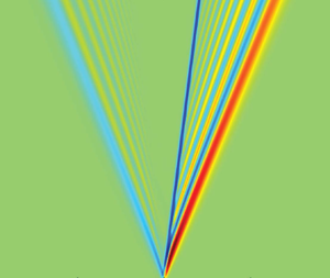
Figure 1.

Side view of the moving seabed deformation system.

$({\rm i})$ Laplace equation

(2.16)\begin{equation} \nabla'^2\varPhi'_{n}=0,\quad \text{in}\ \varOmega(x',z') . \end{equation}

$({\rm ii})$ Free-surface dynamic condition

(2.17)\begin{equation} G'\zeta'+\varPhi'_{t'}=\mathcal{B}_n,\quad z'=0, \end{equation}

where

(2.18a,b)\begin{equation} \mathcal{B}_1=0,\quad \mathcal{B}_2={-}\zeta_1'\varPhi'_{1_{t'z'}}- \tfrac{1}{2}\left|\boldsymbol{\nabla}'\varPhi_1'\right|^2. \end{equation}

$({\rm iii})$ Free-surface mixed condition

(2.19)\begin{equation} \varPhi'_{n_{t't'}}+G'\varPhi'_{n_{z'}}=\mathcal{F}_n,\quad z'=0, \end{equation}

where

(2.20a,b)\begin{equation} \mathcal{F}_1=0,\quad \mathcal{F}_2={-}\zeta_1'(\varPhi'_{1_{t't'z'}}+G'\varPhi'_{1_{z'z'}})- \left|\boldsymbol{\nabla}'\varPhi_1'\right|_{t'}^2. \end{equation}

$({\rm iv})$ Boundary condition at the seabed

(2.21)\begin{equation} \varPhi'_{z'}-f'_{t'}=\mathcal{G}_n,\quad z'={-}h', \end{equation}

where

(2.22a,b)\begin{equation} \mathcal{G}_1=0,\quad \mathcal{G}_2=\varPhi'_{1_{x'}}f'_{x'}-f'\varPhi'_{1_{z'z'}}. \end{equation}

$({\rm v})$ Initial condition

(2.23)\begin{equation} \varPhi_n'=\varPhi'_{n_{t'}}=0,\quad z'=0,\enspace t' = 0^+. \end{equation}

Having obtained the governing equations at each order $n$ we are now in a position to solve each b.v.p. at the leading order $\textit {O}(1)$ and second order $\textit {O}(\epsilon )$.

2.2. Leading-order problem $\textit {O}(1)$

Returning back to physical variables we get the following leading-order problem:

(2.24)\begin{gather} \nabla^2\varPhi_1=0,\quad \varOmega\left(x,z\right), \end{gather}

(2.25)\begin{gather}\varPhi_{1_{tt}}+g\varPhi_{1_z}=0,\quad z=0, \end{gather}

(2.26)\begin{gather}\zeta_1+\frac{1}{g}\varPhi_{1_t}=0,\quad z=0, \end{gather}

(2.27)\begin{gather}\varPhi_{1_z}=f_t,\quad z={-}h, \end{gather}

(2.28)\begin{gather}\varPhi_1=\varPhi_{1_t}=0,\quad z = 0,\enspace t = 0^+. \end{gather}

By applying the Fourier transform along the $x$ coordinate, solving the b.v.p. via separation of variables and transforming back to the spatial variable, we obtain the following expression for the velocity potential:

(2.29)\begin{align} \varPhi_1 &={-}\frac{1}{2{\rm \pi}}\int_0^t\mathrm{d}\tau\int_{-\infty}^\infty \frac{g\cosh\left[k\left(h+z\right)\right]\hat{W}\left(t,k\right) \sin\left[\omega\left(\tau-t\right)\right]{\rm e}^{\mathrm{i}k x}}{\omega\cosh^2(kh)}\,\mathrm{d} k\nonumber\\ &\quad +\frac{1}{2{\rm \pi}}\int_{-\infty}^\infty \frac{\hat{W}\left(t,k\right){\rm e}^{\mathrm{i}kx}\sinh(kz)}{k\cosh(kh)}\,\mathrm{d} k, \end{align}

and the free-surface elevation

(2.30)\begin{equation} \zeta_1=\frac{1}{2{\rm \pi}}\int_0^t\mathrm{d}\tau\int_{-\infty}^\infty \frac{\hat{W}\left(\tau,k\right){\rm e}^{\mathrm{i}kx}\cos \left[\omega\left(\tau-t\right)\right]}{\cosh(kh)}\,\mathrm{d}k,\quad\omega^2=gk\tanh(kh), \end{equation}

where we use the shorthand notation $W(x,\tau ) = f_\tau$, so that

(2.31)\begin{equation} \hat{W}\left(\tau,k\right)=\int_{-\infty}^\infty f_\tau \,{\rm e}^{-\mathrm{i}kx}\,\mathrm{d}\kern0.06em x\end{equation}

is the associated Fourier transform. As an example, let us consider the following analytical expression for the bed perturbation:

(2.32)\begin{equation} f(x,t)=A\exp({-\sigma[x-utH\left(t\right)]^2}),\end{equation}

in which $u$ is the horizontal speed, $\sigma$ is a shape factor, $A$ is the maximum thickness of the perturbed bed and $H(t)$ is the Heaviside step function. Then

(2.33)\begin{equation} f_\tau=2Au\sigma\left[x-u\tau H(\tau)\right] \exp({-\sigma[x-u\tau H(\tau)]^2}) H\left(\tau\right), \end{equation}

and (2.31) becomes

(2.34)\begin{equation} \hat{W}\left(\tau,k\right)={-}\frac{\mathrm{i}Aku\sqrt{\rm \pi} \exp({-[k\left(k+4\mathrm{i}\tau u\sigma \right)/(4\sigma)]}) H\left(\tau\right)}{\sqrt{\sigma}}. \end{equation}

Substitution of (2.34) into (2.30) yields finally

(2.35)\begin{gather} \varPhi_1={-}\frac{g}{2{\rm \pi}}\int_{-\infty}^\infty \frac{{\rm e}^{\mathrm{i}kx}\cosh\left[k\left(h+z\right)\right] }{\omega\cosh^2(kh)}S\left(k,t\right)\mathrm{d} k+ \frac{1}{2{\rm \pi}}\int_{-\infty}^\infty\frac{\hat{W}\left(t,k\right){\rm e}^{\mathrm{i}kx}\sinh(kz)}{k\cosh(kh)}\,\mathrm{d} k, \end{gather}

(2.36)\begin{gather}\zeta_1=\frac{1}{2{\rm \pi}}\int_{-\infty}^\infty\frac{{\rm e}^{\mathrm{i}kx}}{\cosh(kh)}C\left(k,t\right)\mathrm{d} k, \end{gather}

where the terms $C$ and $S$ are, respectively,

(2.37)\begin{gather} C(k,t)={-}\frac{\mathrm{i}Aku\sqrt{\rm \pi}\,{\rm e}^{{-}k^2/(4\sigma)}[\mathrm{i}\,{\rm e}^{-\mathrm{i}ktu}ku-\mathrm{i}ku\cos(\omega t)-\omega\sin(\omega t)]}{(k^2u^2-\omega^2)\sqrt{\sigma}}, \end{gather}

(2.38)\begin{gather}S(k,t)={-}\frac{\mathrm{i}Aku\sqrt{\rm \pi}\,{\rm e}^{{-}k^2/(4\sigma)}[-{\rm e}^{-\mathrm{i}ktu}\omega+\omega\cos(\omega t)-\mathrm{i}ku\sin(\omega t)]}{(k^2u^2-\omega^2)\sqrt{\sigma}}. \end{gather}

Note that $C(-k,t) = \bar {C}(k,t)$ and $S(-k,t)=\bar {S}(k,t)$, where the bar denotes the complex conjugate, hence the integrals in (2.35)–(2.36) are real. They can be evaluated numerically, and the approximation investigated asymptotically for large times and distance from $x=0$, as described in § 4. Use of (2.36)–(2.37) yields the following analytical expression of the free-surface elevation in integral form:

(2.39)\begin{equation} \zeta_1={-}\frac{\mathrm{i}Au}{2\sqrt{{\rm \pi} \sigma}}\int_{-\infty}^\infty \frac{k\exp({\mathrm{i}kx-k^2/(4\sigma)})[\mathrm{i}\,{\rm e}^{-\mathrm{i}ktu}ku-\mathrm{i}ku \cos(\omega t)-\omega\sin(\omega t)]}{(k^2u^2-\omega^2)\cosh(kh)}\mathrm{d} k.\end{equation}

2.3. Second-order problem $\textit {O}(\epsilon )$

The second-order problem expressed in terms of physical variables is given by

(2.40a,b)\begin{equation} \nabla^2\varPhi_2=0,\quad \varOmega\left(x,z\right), \end{equation}

(2.41)\begin{align} & \varPhi_{2_{tt}}+g\varPhi_{2_z} \nonumber\\ &\quad ={-}\frac{1}{\epsilon}[\zeta_1(\varPhi_{1_{ttz}}+g\varPhi_{1_{zz}})-2g \varPhi_{1_x}\zeta_{1_x}+2\varPhi_{1_{zt}}\zeta_{1_t}]=F\left(x,t\right),\quad z=0, \end{align}

(2.42)\begin{gather} \zeta_2+\frac{1}{g}\varPhi_{2_t}={-}\frac{1}{\epsilon}\left[\frac{1}{2g} (\varPhi_{1_x}^2+\zeta_{1_t}^2)+ \frac{\varPhi_{1_{zt}}\zeta_1}{g}\right]=B\left(x,t\right),\quad z=0, \end{gather}

(2.43)\begin{gather}\varPhi_{2_z}=\frac{1}{\epsilon}(-\varPhi_{1_{zz}}f+ \varPhi_{1_x}f_x)=G\left(x,t\right),\quad z={-}h, \end{gather}

(2.44)\begin{gather}\varPhi_2=\varPhi_{2_t}=0,\quad z = 0,\enspace t = 0^+. \end{gather}

To determine the free-surface elevation $\zeta _2$, we decompose the second-order velocity potential as $\varPhi _2=\varPhi _F+\varPhi _G$, where $\varPhi _F$ represents the solution forced at the free surface, while $\varPhi _G$ represents the solution forced by the bed motion. This implies that $f(x,t)$ cannot have edges leading to infinite velocity, because the second-order solution would otherwise become unbounded. In addition, we decompose the free-surface elevation $\zeta _2$ into three components, namely $\zeta _2=\zeta _F+\zeta _G+B$, where $B=B(x,t)$ represents the second-order forcing of the first-order solution, defined in (2.42). For later convenience, we include all the components of each forcing term $G, F$ and $B$, in Appendix A.

We now proceed to solve each component separately.

2.3.1. Second-order free-surface forcing term

The set of governing equations is given by

(2.45)\begin{gather} \nabla^2\varPhi_F=0,\quad \varOmega\left(x,z\right), \end{gather}

(2.46)\begin{gather}\varPhi_{F_{tt}}+g\varPhi_{F_z}=F\left(x,t\right),\quad z=0, \end{gather}

(2.47)\begin{gather}\zeta_F+\frac{1}{g}\varPhi_{F_t}=0,\quad z=0, \end{gather}

(2.48)\begin{gather}\varPhi_{F_z}=0,\quad z={-}h, \end{gather}

(2.49)\begin{gather}\varPhi_F=\varPhi_{F_t}=0,\quad z = 0,\enspace t = 0^+. \end{gather}

A solution can be sought by applying the Fourier transform along the $x$ coordinate. We obtain

(2.50)\begin{equation} \varPhi_F=\frac{1}{2{\rm \pi}}\int_0^t\int_{-\infty}^\infty \frac{\cosh{[k\left(h+z\right)]}\hat{F}\left(\tau,k\right){\rm e}^{\mathrm{i}kx} \sin{[\omega\left(\tau-t\right)]}}{\omega\cosh(kh)}\mathrm{d} k\,\mathrm{d}\tau, \end{equation}

where $\hat {F}(t,k)$ is the Fourier transform of the forcing term on the free surface (see (2.41)).

By applying the Leibniz integral rule to (2.50), we obtain the free-surface elevation $\zeta _F$ given by the effect of the forcing terms on the free surface:

(2.51)\begin{equation} \zeta_F\left(x,t\right)={-}\frac{1}{2g{\rm \pi}}\int_0^t\int_{-\infty}^\infty \int_{-\infty}^\infty F\left(\tau,\xi\right)\exp\left({-\mathrm{i}k\left(\xi-x\right)}\right) \cos\left[\omega\left(\tau-t\right)\right]\mathrm{d}\xi\,\mathrm{d} k\,\mathrm{d}\tau. \end{equation}

The latter can be evaluated numerically for given values of the horizontal coordinate $x$ and time $t$.

2.3.2. Second-order bed forcing term

The b.v.p. is

(2.52)\begin{gather} \nabla^2\varPhi_G=0,\quad \varOmega\left(x,z,t\right), \end{gather}

(2.53)\begin{gather}\varPhi_{G_{tt}}+g\varPhi_{G_z}=0,\quad z=0, \end{gather}

(2.54)\begin{gather}\zeta_G+\frac{1}{g}\varPhi_{G_t}=0,\quad z=0, \end{gather}

(2.55)\begin{gather}\varPhi_{G_z}=G\left(x,t\right),\quad z={-}h, \end{gather}

(2.56)\begin{gather}\varPhi_G=\varPhi_{G_t}=0,\quad z=0,\enspace t = 0^+. \end{gather}

The solution is formally equivalent to that derived at leading order. We obtain the forced second-order potential,

(2.57)\begin{align} \varPhi_G&={-}\frac{1}{2{\rm \pi}}\int_0^t\int_{-\infty}^\infty \frac{g\cosh{[k\left(h+z\right)]}\hat{G}\left(t,k\right){\rm e}^{\mathrm{i}kx} \sin{[\omega\left(\tau-t\right)]}}{\omega\cosh^2(kh)}\mathrm{d}k\,\mathrm{d}\tau\nonumber\\ &\quad +\frac{1}{2{\rm \pi}}\int_{-\infty}^\infty \frac{\hat{G}\left(t,k\right){\rm e}^{\mathrm{i}kx}\sinh(kz)}{k\cosh(kh)}\mathrm{d} k, \end{align}

where $\hat {G}$ is the Fourier transform of the forcing term at the bed, $G(x,t)$.

Similar to the previous section, the corresponding free-surface elevation is derived upon application of the Leibniz integral rule, which yields

(2.58)\begin{equation} \zeta_G\left(x,t\right)=\frac{1}{2{\rm \pi}}\int_0^t\int_{-\infty}^\infty \int_{-\infty}^\infty \frac{G\left(\tau,\xi\right)\exp\left({-\mathrm{i}k\left(\xi-x\right)}\right) \cos\left[\omega\left(\tau-t\right)\right]}{\cosh(kh)}\mathrm{d}\xi\,\mathrm{d} k\,\mathrm{d}\tau. \end{equation}

The sought solution for the free-surface elevation is given by

(2.59)\begin{equation} \zeta(x,t) = \zeta_1(x,t) + \epsilon\left[\zeta_F(x,t)+\zeta_G(x,t)+B(x,t) \right] + O(\epsilon^2).\end{equation}

3.1. Experimental set-up

Experiments were undertaken in a flume of 0.25 m width and 14.66 m length. Waves were generated by a semi-ellipsoidal moving block of length $L=0.5$ m and height $A=0.026$ m sliding on a horizontal seabed, at a depth $h=0.175$ m. Use of a horizontal boundary and the location of the block near the centre of the flume (i.e. approximately equidistant from the flume ends) ensured that waves propagating in both positive and negative directions could be measured prior to reflection. No wave absorption material was present at the ends of the flume. The experimental set-up is described in detail by Whittaker et al. (Reference Whittaker, Nokes and Davidson2015).

The block motion (provided by a servo motor) comprised an initial acceleration at a constant rate $a_0=1.5$ ms$^{-2}$ until $t=0.109$ s, when the block reached its maximum velocity of $u=0.164$ ms$^{-1}$. This is similar to Run 5 reported by Whittaker et al. (Reference Whittaker, Nokes and Davidson2015), and corresponds to a landslide Froude number of 0.125. However, in the experiments undertaken by Whittaker et al. (Reference Whittaker, Nokes and Davidson2015), the landslide moved at its maximum velocity for 2.00 s before decelerating to rest (with a deceleration of $-a_0$). In these experiments, the landslide block did not decelerate during the measurement period. In other words, the block motion consisted of an initial rapid acceleration followed by a long period of constant velocity. Whittaker et al. (Reference Whittaker, Nokes, Lo, Liu and Davidson2017) present a similar wave field for a Froude number of $0.5$, but did not include wave fields generated at lower Froude numbers. The rapid block acceleration, relatively low maximum velocity (i.e. Froude number) and lack of deceleration make these experimental results suitable for theoretical comparisons because the block movement matches the assumptions in (2.32).

In the experiments carried out by Whittaker et al. (Reference Whittaker, Nokes and Davidson2015,  Reference Whittaker, Nokes, Lo, Liu and Davidson2017), free-surface elevations were measured within a spatial window of approximately 0.35 m using a laser-induced fluorescence technique to an accuracy of $\pm$4 mm. The highly repeatable block motion allowed the full wave field to be measured through 37 repetitions of the experiment, ensuring some overlap between adjacent fields of view to create a continuous free-surface record.

3.2. Analytical vs experimental results

Now we compare analytical results with data from the experimental campaign outlined above. Water depth and landslide velocity are the same as in the previous section, the bed deformation maximum thickness is $A=0.026\,\mathrm {m}$ and the shape factor representing the moving block is $\sigma =19\,\mathrm {m}^{-2}$. Although subtle differences exist between the shape of the block in the experiments and analytical model, previous research (e.g. Sue et al. Reference Sue, Nokes and Davidson2011; Whittaker et al. Reference Whittaker, Nokes and Davidson2015) has demonstrated that acceptable agreement can be obtained if the volumes are equal. The analytical domain also extends to infinity on both sides, whereas the experimental set-up is $14.66\,\mathrm {m}$ long. Figure 2 shows snapshots of the free-surface elevation $\zeta$ obtained with the second-order and leading-order models. On the same figure the free-surface elevation evaluated experimentally (dashed line) is also plotted. A pronounced leading wave travels ahead of the solid block, while a trough propagates in the opposite direction. Both waves are followed by trailing wave packets that resemble the Airy wave solution discussed later in § 4. The times of arrival of crests and troughs, as well as the overall shape of the wave patterns are in close agreement between the two models. Slight differences in the profiles appear at small times, where the leading wave and the trough are underestimated by the analytical model. Note that at small times the dynamics is highly nonlinear, as the bed deformation imparts a sudden impulse to the surrounding fluid when its speed changes from $u=0$ for $t<0$ to $u>0$ for $t\geq 0$. Also, the moving block velocity in the experimental set-up increases gradually until $t=0.109$ s, whereas the velocity of the moving bed slide for the theoretical model is described by the Heaviside step function as shown by (2.32). Therefore, the small differences between the analytical and experimental models (i.e. the over-estimation of wave amplitudes in the second-order solution) are likely due to the effects highlighted above. Interestingly, the leading-order solution $\zeta _1$ still underestimates the amplitudes of the generated waves, despite the instantaneous acceleration assumed in this model, reinforcing the importance of the second-order contributions to the generated wave field. Note also that at large times there are discrepancies in front of the leftward propagating trough. This is due to the near-complete wave reflection caused by the presence of the vertical wall on the left side of the channel flume, whereas the fluid domain for the analytical model extends to infinity. Reflections from this boundary were first observed at approximately $t=1.6$ s in the physical experiments (Whittaker et al. Reference Whittaker, Nokes and Davidson2015).

Figure 2.

Second-order free-surface elevation $\zeta _2+\zeta _1$, leading-order free-surface elevation $\zeta _1$ and experimental data at times: (a) $t = 0.5\,\mathrm {s}$, (b) $t = 1\,\mathrm {s}$, (c) $t = 1.5\,\mathrm {s}$ and (d) $t=2\,\mathrm {s}$, (e) $t = 2.5\,\mathrm {s}$ and (f) $t=3\,\mathrm {s}$. The agreement between the models is good with few discrepancies at the initial stage. This is likely due to the instantaneous acceleration not possible in the experimental set-up.

4.1. Rightward leading wave at first order

In this section we derive the profile of the rightward leading wave; the asymptotic behaviour of the leftward propagating trough can be found in a similar manner.

First, we note that the contribution given by the first term within the square brackets in (2.39) is negligible, because the integral has no stationary points (Mei et al. Reference Mei, Stiassnie and Yue2005). The free-surface elevation at large distances can consequently be approximated as

(4.1) \begin{align} \zeta_1^\infty&\simeq{-}\frac{Au}{\sqrt{{\rm \pi} \sigma}}\int_{0}^\infty \frac{\exp({-k^2/(4\sigma)})[k^2 u\cos{kx}\cos(\omega t)+ \omega k\sin{kx}\sin(\omega t)] }{(k^2u^2-\omega^2)\cosh(kh)}\mathrm{d} k\nonumber\\ &={-}\frac{Au}{2\sqrt{{\rm \pi} \sigma}}Re\int_{0}^\infty\frac{\begin{array}{l} \exp({-k^2/(4\sigma)})[k^2 u\left(\exp\left({\mathrm{i}\left(kx-\omega t\right)}\right)+ \exp\left({\mathrm{i}\left(kx+\omega t\right)}\right)\right) \\ \quad +\omega k\left(\exp\left({\mathrm{i}\left(kx-\omega t\right)}\right)- \exp\left({\mathrm{i}\left(kx+\omega t\right)}\right)\right)] \end{array}}{(k^2u^2-\omega^2)\cosh(kh)}\mathrm{d} k. \end{align}

The first and second terms within each round bracket of the numerator represent rightward and leftward propagating waves, respectively. Given that rightward leading waves are located at $x>0$, the integral including $\exp \{\mathrm {i}(kx+\omega t)\}$ does not have a stationary point and provides a negligible contribution (Bender & Orszag Reference Bender and Orszag1999). Hence, only the integral including the first complex exponential $\exp \{\mathrm {i}(kx-\omega t)\}$ is of significance. We obtain

(4.2) \begin{align} \zeta_1^\infty &\simeq{-}\frac{Au}{2\sqrt{{\rm \pi} \sigma}}Re \int_{0}^\infty\frac{k\exp({-k^2/(4\sigma)+\mathrm{i}\left(kx-\omega t\right)}) (k u+\omega)}{(k^2u^2-\omega^2)\cosh(kh)}\mathrm{d}k \nonumber\\ &= \int_{0}^\infty\tilde{\zeta}(k)\cos\left(kx-\omega t\right)\mathrm{d}k. \end{align}

Note that leading waves move at speeds close the shallow-water celerity $\sqrt {g h}$ and correspond to small wavenumbers $k\sim 0$. To investigate the latter integral analytically, let us expand $\omega$ about $k\rightarrow 0$ and take into account wave dispersion up to the third power:

(4.3)\begin{equation} \omega\simeq\sqrt{gh}k\left(1-\frac{h^2k^2}{6}\right). \end{equation}

Substitution of (4.3) into (4.2) yields

(4.4)\begin{equation} \zeta_1^\infty\simeq\int_{0}^\infty\tilde{\zeta}(k)\cos \left[k\big(x-t\sqrt{gh}\big)+k^3\frac{\sqrt{gh}h^2 t}{6}\right]\mathrm{d} k. \end{equation}

The latter integral can be further simplified by Taylor expanding $\tilde {\zeta }$ about $k\rightarrow 0$ and considering the first-order term (Whitham Reference Whitham1974; Debnath Reference Debnath1994; Mei et al. Reference Mei, Stiassnie and Yue2005)

(4.5)\begin{equation} \zeta_1^\infty\simeq\frac{Au}{2\big(\sqrt{gh}-u\big)\sqrt{{\rm \pi} \sigma}} \int_0^\infty\cos\left[k\big(x-t\sqrt{gh}\big)+\frac{th^2k^3\sqrt{gh}}{6}\right]\mathrm{d}k. \end{equation}

Let us now substitute the following variables:

(4.6a,b) \begin{equation} Z\alpha=k\big(x-\sqrt{gh}t\big),\quad Z^3=\frac{2\big(x-\sqrt{gh}t\big)^3}{\sqrt{gh}h^2t} . \end{equation}

This yields

(4.7)\begin{equation} \zeta_1^\infty\simeq\frac{A\sqrt{\rm \pi}Fr}{2\left(1-Fr\right)\sqrt{\sigma}} \left(\frac{2}{h^2t\sqrt{gh}}\right)^{{1}/{3}}\text{Ai}\left[\left(\frac{2}{h^2t\sqrt{gh}}\right)^{{1}/{3}} \big[x-t\sqrt{gh}\big]\right], \end{equation}

where $\textrm {Ai}$ is Airy's function and $Fr=u/\sqrt {gh}$ is the Froude number of the disturbance. For an observer travelling at a speed close to the long-wave speed $\sqrt {gh}$, the leading wave $\zeta _1^\infty$ decays as $O(t^{-1/3})$. This rate of decay is the same as that of transient waves generated by an initial displacement of the free surface (Mei et al. Reference Mei, Stiassnie and Yue2005).

Note that (4.7) is proportional to the volume of the disturbance $A\sqrt {{\rm \pi} }/\sqrt {\sigma }$, and that it becomes unbounded as $Fr\rightarrow 1$, i.e. as the disturbance speed tends to the wave speed in shallow water $\sqrt {gh}$. The same result is also obtained in the case of surface waves on a running stream and has been investigated by several authors (Whitham Reference Whitham1974; Wu Reference Wu1987; Lee et al. Reference Lee, Yates and Wu1989; Debnath Reference Debnath1994).

4.2. Free-surface elevation in the disturbance region at the leading order

To analyse the free-surface elevation in the disturbance region behind the leading wave, let us split (2.39) into two components, $\zeta _1=\zeta _1^s+\zeta _1^w$, where $\zeta _1^s$ represents a stationary free-surface elevation in the moving reference frame $X=x-u t$, and $\zeta _1^w$ denotes an oscillating part.

Let us start with the stationary component, i.e.

(4.8) \begin{equation} \zeta_1^s=\frac{Au^2}{2\sqrt{{\rm \pi} \sigma}}\int_{-\infty}^\infty \frac{k^2\exp({\mathrm{i}kX-k^2/(4\sigma)})}{(k^2u^2-\omega^2)\cosh(kh)}\mathrm{d} k. \end{equation}

The latter integral cannot be investigated via the stationary phase method because the term $X$ is insufficiently large in the landslide region. However, the integral can be investigated analytically by noting that the term $\exp \{-k^2/(4\sigma )\}$ governs the leading behaviour of the integrand in $k\sim 0$. Hence, by Taylor expanding the integrand about $k\rightarrow 0$, except for the exponential terms, we obtain

(4.9)\begin{equation} \zeta_1^s\simeq{-}\frac{Au^2}{2\sqrt{{\rm \pi} \sigma}(gh-u^2)} \int_{-\infty}^\infty \exp({\mathrm{i}kX-k^2/(4\sigma)})\,\mathrm{d} k={-}\frac{Au^2\,{\rm e}^{{-}X^2\sigma}}{(gh-u^2)}={-}\frac{f(X) Fr^2}{(1-Fr^2)}. \end{equation}

Retaining the exponential terms, instead of including them in the Taylor expansion, allows us to find the dependence on the moving coordinate $X$ and to improve the accuracy of the approximated solution of (4.9). From (4.9) we note that the solution becomes unbounded as $Fr\rightarrow 1$, whereas if the seabed velocity is smaller than the wave speed in shallow water, i.e. $Fr<1$, the free-surface elevation develops a trough of permanent shape moving with the seabed deformation at speed $u$. This result for the first-order stationary component $\zeta _1^s$ is identical to the well-known result for long waves (Levin & Nosov Reference Levin and Nosov2016). Similar behaviour has also been observed experimentally by Whittaker et al. (Reference Whittaker, Nokes and Davidson2015) and in the experimental results provided in figure 2.

The oscillating part $\zeta _1^w$ can be investigated by using the method of stationary phase (Mei et al. Reference Mei, Stiassnie and Yue2005). From (4.2) we obtain

(4.10) \begin{align} \zeta_1^w&={-}\frac{Au}{2\sqrt{{\rm \pi} \sigma}}Re\int_{0}^\infty \frac{k\exp({-k^2/(4\sigma)+\mathrm{i}\left(kx-\omega t\right)})(k u+\omega)}{(k^2u^2-\omega^2)\cosh(kh)}\mathrm{d}k\nonumber\\ &\simeq{-}\frac{Au}{\sqrt{2 \sigma t\left|\omega''_0\right|}}\frac{k_0\exp({-k_0^2/(4\sigma)})}{(k_0u-\omega_0)\cosh\left(k_0h\right)} \cos{\left(k_0x-\omega_0t+\frac{\rm \pi}{4}\right)}, \end{align}

where $k_0$ is the stationary point satisfying $x/t=\mathrm {d}\omega /\mathrm {d}k$, and $\omega _0$ is the frequency evaluated at $k_0$. For deeper physical insight, let us now consider the Boussinesq expansion (4.3) and consider an observer moving together with the bed deformation, i.e. $x=ut$. The explicit expressions for $k_0$ and $\omega ''_0=\mathrm {d}^2\omega /\mathrm {d}k^2|_{k_0}$ simplify as

(4.11a,b)\begin{equation} k_0=\frac{\sqrt{2\left(1-Fr\right)}}{h},\quad \omega''_0={-}h^2k_0\sqrt{gh}={-}h\sqrt{2gh\left(1-Fr\right)}, \end{equation}

respectively. Substituting (4.11a,b) back into (4.10), we obtain

(4.12)\begin{equation} \zeta_1^w\simeq\frac{3Au\exp({-k_0^2/(4\sigma)})}{2^{{7}/{4}} \left(1-Fr\right)^{{5}/{4}}\left(gh\right)^{{3}/{4}}\sqrt{\sigma h t}\cosh\left(k_0h\right)} \cos{\left[\frac{2t\sqrt{2gh}\left(1-Fr\right)^{{3}/{2}}}{3h}-\frac{\rm \pi}{4}\right]},\end{equation}

i.e. the observer sees a train of waves decaying as $\textit {O}(t^{-1/2})$ and travelling rightwards along the trough (4.9), with relative phase speed

(4.13)\begin{equation} c=u-\frac{\omega_0}{k_0}=\frac{2\sqrt{gh}}{3}\left(1-Fr\right). \end{equation}

Note that as $t\rightarrow \infty$ only the stationary component $\zeta _1^s$ survives.

As outlined by Schäffer & Madsen (Reference Schäffer and Madsen1995) and Kirby (Reference Kirby2016), the expansion (4.3) can be further improved to approximate the frequency $\omega$ even in the case of large wavenumber $k$. However, the stationary point $k_0$ would not have an explicit expression anymore and numerical methods are required to evaluate the solution. Given that our scope is to find explicit, approximate expressions for the free-surface elevation, we retain terms up to third order and continue to adopt the classical Boussinesq expansion (4.3).

4.3. Second-order term $\zeta _G$

To investigate the behaviour of the forcing term $G$ inside the expression for $\zeta _G$ (2.58), we first analyse the component $\varPhi _{zz} f$, where $\varPhi _{zz}$ is defined by (A7) and $f$ represents the bed deformation (2.32). The shape function $f$ is governed by an exponential term associated with forcing in the landslide region $X\sim 0$, and so we expect that oscillatory components far from the perturbation make small contributions. The steady component in $\varPhi _{zz}$ reads

(4.14)\begin{align} \varPhi_{1_{zz}} &={-}\frac{\mathrm{i}Au}{2\sqrt{{\rm \pi}\sigma}} \int_{-\infty}^\infty\frac{k^3 \exp({\mathrm{i}k(x-ut)-k^2/(4\sigma)})}{(k^2u^2-\omega^2)\cosh^2(kh)}\mathrm{d}k \nonumber\\ &\quad +\frac{\mathrm{i}Au}{2 g\sqrt{{\rm \pi}\sigma}} \int_{-\infty}^\infty k\omega^2\exp({\mathrm{i}k(x-ut)-k^2/(4\sigma)})\,\mathrm{d} k. \end{align}

The latter integrals can be investigated analytically by noting that the exponential $\exp \{-k^2/(4\sigma )\}$ focuses the contributions as $k\rightarrow 0$. As before, we retain the complex exponential to improve the approximation, but Taylor expand the other terms about $k\rightarrow 0$. Hence,

(4.15)\begin{align} \varPhi_{1_{zz}}&\simeq{-}\frac{\mathrm{i}Au}{2\sqrt{{\rm \pi}\sigma} (u^2-gh)}\int_{-\infty}^\infty k \exp({\mathrm{i}k(x-ut)-k^2/(4\sigma)})\,\mathrm{d}k \nonumber\\ &\quad +\frac{\mathrm{i}Auh}{2 \sqrt{{\rm \pi}\sigma}}\int_{-\infty}^\infty k^3 \exp({\mathrm{i}k(x-ut)-k^2/(4\sigma)})\,\mathrm{d}k \nonumber\\ &={-}\frac{2f(X)u\sigma X}{h}\left\{\frac{1}{1-Fr^2}+2h^2\sigma[3-2\sigma X^2] \right\}, \end{align}

which models a rightwards propagating trough followed by a single crest. Similarly, we derive the steady component of $\varPhi _x$ (A8) which is part of the forcing term $\varPhi _x f_x$ in $G$ as

(4.16)\begin{align} \varPhi_{1_{x}} &={-}\frac{Aug}{2\sqrt{{\rm \pi}\sigma}}\int_{-\infty}^\infty \frac{k^2 \exp({\mathrm{i}k(x-ut)-k^2/(4\sigma)})}{(k^2u^2-\omega^2)\cosh^2(kh)}\mathrm{d}k \nonumber\\ &\quad -\frac{Au}{2g\sqrt{{\rm \pi}\sigma}}\int_{-\infty}^\infty\omega^2 \exp({\mathrm{i}k(x-ut)-k^2/(4\sigma)})\,\mathrm{d} k. \end{align}

Again, we retain the complex exponential and Taylor expand the integrands about $k\rightarrow 0$,

(4.17)\begin{align} \varPhi_{1_{x}}&\simeq{-}\frac{Aug}{2\sqrt{{\rm \pi}\sigma}(u^2-gh)} \int_{-\infty}^\infty \exp({\mathrm{i}k(x-ut)-k^2/(4\sigma)})\,\mathrm{d}k \nonumber\\ &\quad -\frac{Auh}{2\sqrt{{\rm \pi}\sigma}}\int_{-\infty}^\infty k^2 \exp({\mathrm{i}k(x-ut)-k^2/(4\sigma)})\,\mathrm{d}k \nonumber\\ &={-}\frac{f(X)u}{h}\left\{\frac{1}{1-Fr^2}+2h^2\sigma[1-2\sigma X^2]\right\}, \end{align}

which represents a propagating trough. Therefore, the forcing term $G$ (2.43) can be approximated as

(4.18) \begin{equation} G\simeq\frac{4u\sigma f^2X[1+4h^2\sigma(1-Fr^2) (1-\sigma X^2)]}{\epsilon h (1-Fr^2)}. \end{equation}

Use of the expression for $\zeta _G$ (2.58) yields

(4.19) \begin{equation} \zeta_G=\frac{A}{8{\rm \pi}\sqrt{2}h(1-Fr^2)}\int_{-\infty}^{\infty} \frac{\exp({\mathrm{i}kx+k^2/(8\sigma)})C}{\cosh(kh)}[4+h^2(1-Fr^2)(k^2+4\sigma)]\mathrm{d}k. \end{equation}

Let us first define the rightward leading wave approximation of the term above as $\zeta _G^\infty$. By expanding the integrand except for the phase functions and recalling that terms proportional to $\exp \{\mathrm {i}(kx+\omega t)\}$ give negligible contributions we obtain

(4.20) \begin{align} \zeta_G^\infty &\simeq{-}\frac{A^2[hu^2\sigma-g(1+h^2\sigma)]}{2\sqrt{2{\rm \pi}\sigma} (u^2-gh)^2}\int_0^{\infty}\cos(kx-\omega t)\mathrm{d}k \nonumber\\ &=\frac{A}{h\sqrt{2}}\left(h^2\sigma+\frac{1}{1-Fr^2}\right)\times\zeta_1^\infty, \end{align}

where $\zeta _1^\infty$ is the leading wave approximation at the leading order (4.7). The term in rounded brackets is positive for small Froude numbers, thus $\zeta _G^\infty$ causes the amplitude of the leading wave to increase. This second-order contribution depends on three main parameters: (i) the ratio of disturbance height (or wave amplitude scale) to offshore water depth $A/h$; (ii) the Froude number $Fr$; and (iii) the ratio between water depth $h$ and bed perturbation length scale $1/\sqrt {\sigma }$. Therefore, the second-order solution forced at the free surface is valid so long as the ratio $A/h$ and $h\sqrt {\sigma }$ are both small and $Fr\ll 1$, i.e. away from the critical speed.

In the landslide region, a different approximation is required. We write $\zeta _G=\zeta _G^s+\zeta _G^w$, where the superscripts refer to the static and oscillatory components in $C$. We obtain

(4.21) \begin{align} \zeta_G^s&=\frac{A^2u^2}{8h\sqrt{2{\rm \pi}\sigma}(1-Fr^2)} \int_{-\infty}^{\infty}\frac{\exp({\mathrm{i}kX-k^2/(8\sigma)})k^2 [4+h^2(1-Fr^2)(k^2+4\sigma)]}{(k^2u^2-\omega^2)\cosh(kh)}\mathrm{d}k\nonumber\\ &\simeq{-}\frac{f^2Fr^2}{h(1-Fr^2)}\left(h^2\sigma+\frac{1}{1-Fr^2}\right)= \frac{f}{h}\left(h^2\sigma+\frac{1}{1-Fr^2}\right)\times\zeta_1^s, \end{align}

in which we have adopted an approximation for $k\sim 0$ because of the exponential term $\exp \{-k^2/(8\sigma )\}$. Therefore, the effect of $\zeta _G^s$ is to increase the depth trough; indeed the latter is proportional to the square of landslide shape $f^2$ and increases with $Fr$.

The second and third terms in $C$ represent the oscillatory component leading to $\zeta _G^w$, which is investigated by applying the stationary phase method as follows:

(4.22) \begin{align} \zeta_G^w&\simeq{-}\frac{A^2uk_0\exp({-k_0^2/(8\sigma)})[4+h^2(1-Fr^2) (k_0^2+4\sigma)]}{8\sqrt{2{\rm \pi}\sigma}h(1-Fr^2)(k_0u-\omega_0)\cosh(k_0h)} \nonumber\\ &\quad \times\cos[k_0x-\omega_0t+\frac{\rm \pi}{4}]\sqrt{\frac{2{\rm \pi}}{t\left|\omega_0^{''}\right|}} \nonumber\\ &=\frac{A\exp({k_0^2/(8\sigma)})}{h\sqrt{2}}\left(\frac{1}{1-Fr^2}+ \frac{h^2(k_0^2+4\sigma)}{4}\right)\times\zeta_1^w, \end{align}

which is in phase with $\zeta _1^w$ (4.10) and so makes a positive contribution. Note that for $k_0\rightarrow 0$ we recover the same term multiplying $\zeta _1^\infty$ in (4.20).

4.4. Second-order term $\zeta _F$

As is demonstrated in the following section, the term $\zeta _F$ is characterised by narrow fluctuations between the leading waves and the landslide region. Given that these oscillations occur along the $x$-coordinate we expect that among all the forcing terms included in $F$, those including the $x$-derivatives provide the most significant contributions. For this reason, we focus solely on the behaviour of $\varPhi _x\zeta _x$ and investigate how this term affects the second-order component $\zeta _F$.

From (4.9)–(4.10), we note that away from the leading waves, the spatial derivative of the free surface indicates that it is composed of a stationary shape moving with the bed deformation and an oscillating part as follows:

(4.23)\begin{equation} \zeta_{1_x}\simeq\frac{2\sigma XfFr^2}{1-Fr^2}+\frac{Au}{\sqrt{2 \sigma t\left|\omega''_0\right|}} \frac{k_0^2\exp({-k_0^2/(4\sigma)})}{\left(k_0u-\omega_0\right)\cosh\left(k_0h\right)} \sin{\left(k_0x-\omega_0t+\frac{\rm \pi}{4}\right)} =\zeta_{1_x}^s+\zeta_{1_x}^w.\end{equation}

Similarly, the velocity potential derivative $\varPhi _{1_x}$ is approximated by

(4.24)\begin{align} \varPhi_{1_x}&\simeq{-}\frac{uf}{h(1-Fr^2)}-\frac{Aug}{\sqrt{2 \sigma t\left|\omega''_0\right|}} \frac{k_0^2\,{\rm e}^{{-}k_0^2/(4\sigma)} }{\left(k_0u-\omega_0\right)\omega_0\cosh\left(k_0h\right)} \cos{\left(k_0x-\omega_0t+\frac{\rm \pi}{4}\right)}\nonumber\\ &=\varPhi_{1_x}^s+\varPhi_{1_x}^w. \end{align}

Therefore the corresponding free-surface elevation $\zeta _F$ reads

(4.25)\begin{equation} \zeta_F\left(x,t\right)\simeq{-}\frac{1}{\rm \pi}\int_0^t\int_{-\infty}^\infty \int_{-\infty}^\infty\zeta_{1_\xi}\varPhi_{1_{\xi}}\exp\left({-\mathrm{i}k\left(\xi-x\right)}\right) \cos{\omega\left(\tau-t\right)}\,\mathrm{d}\xi\,\mathrm{d} k\,\mathrm{d}\tau. \end{equation}

The forcing component $\zeta _{1_\xi }^w\varPhi _{1_\xi }^w$ in the integral above, decays as $O(t^{-1})$, i.e. much faster than $\zeta _{1_\xi }^s\varPhi _{1_\xi }^s$, $\zeta _{1_\xi }^w\varPhi _{1_\xi }^s$ and $\zeta _{1_\xi }^s\varPhi _{1_\xi }^w$, and so makes a negligible contribution.

Recalling that $\zeta _1=\zeta _{1_x}^s+\zeta _{1_x}^w$, accordingly we write $\zeta _F=\zeta _F^{s}+\zeta _F^{sw}$, where the superscripts indicate the contributions of static ($\zeta _{1_\xi }^s\varPhi _{1_\xi }^s$) and product between oscillating and static components $(\zeta _{1_\xi }^s\varPhi _{1_\xi }^w;\zeta _{1_\xi }^w\varPhi _{1_\xi }^s)$, respectively, to the second-order term (4.25). The contribution of $\zeta _{1_\xi }^s\varPhi _{1_\xi }^s$ yields

(4.26)\begin{align} \zeta_F^s &\simeq\frac{2A^2gu^3\sigma}{{\rm \pi}(gh-u^2)^2}\int_0^t \int_{-\infty}^\infty\int_{-\infty}^\infty \exp({-\mathrm{i}k(\xi-x)-2(\xi-u\tau)^2\sigma}) \nonumber\\ &\quad \times \left(\xi-\tau u\right)\cos{[\omega\left(\tau-t\right)]} \mathrm{d}\xi\,\mathrm{d} k\,\mathrm{d}\tau \nonumber\\ &=\frac{Au^2g}{2{\rm \pi}\sqrt{2}(u^2-gh)^2} \int_{-\infty}^\infty \exp({\mathrm{i}kx+k^2/(8\sigma)})C\left(k,t\right)\mathrm{d}k. \end{align}

If we focus attention on the leading wave, the primary contribution is given by $k\sim 0$, hence the integral above can be approximated as

(4.27)\begin{align} \zeta_F^{s,\infty} &\simeq \frac{A^2u^3g\sqrt{\rm \pi}}{2{\rm \pi}\sqrt{2\sigma}(u^2-gh)^2(\sqrt{gh}-u)} \nonumber\\ &\quad \times Re\int_{0}^\infty\cos{\left(kx-\omega t\right)}\mathrm{d}k= \frac{AF\,r^2}{\sqrt{2}h(Fr^2-1)^2}\times\zeta_1^\infty, \end{align}

which causes the amplitude of the leading wave to increase. The second-order contribution of (4.27) depends on two main parameters: (i) the ratio of disturbance height (or wave amplitude scale) to offshore water depth $A/h$; and (ii) the Froude number $Fr$. Therefore, the second-order solution forced at the free surface is valid so long as the ratio $A/h$ is small and $Fr<1$, i.e. away from the critical speed. Note also that for small Froude numbers (4.27) is much smaller than the second-order leading wave component $\zeta _G^\infty$ (4.20). In this work $Fr\ll 1$ and so $\zeta _F^{s,\infty }$ makes a small contribution to the leading wave behaviour. If we now focus on the disturbance region, performing a similar analysis as in § 4.2 on expression (4.26) yields $\zeta _F^s = \zeta _F^{s,s}+\zeta _F^{s,w}$, where

(4.28) \begin{equation} \zeta_F^{s,s}\simeq\frac{A^2u^4g}{2\sqrt{2}(u^2-gh)^3\sqrt{\sigma {\rm \pi}}} \int_{-\infty}^\infty \exp({[\mathrm{i}kX-k^2/(8\sigma)]})\mathrm{d} k={-}\frac{f^2Fr^4}{h(1-Fr^2)^3}. \end{equation}

Therefore, the effect of $\zeta _F^{s,s}$ is to increase the depth of the trough and to reduce its width. This term is mainly related to the shape $f$ and speed $u$ of the moving deformation and gives insignificant results when $Fr\ll 1$.

It remains to investigate the term $\zeta _F^{s,w}$ given by the remaining contribution to $C$. From (4.26), the stationary phase method gives

(4.29)\begin{equation} \zeta_F^{s,w}=\frac{AFr^2\exp({k_0^2/(8\sigma)}) \cosh{(k_0h)}}{h\sqrt{2}(1-Fr^2)}\times \zeta_1^w, \end{equation}

which is small for bed deformation speeds far from the shallow-water wave celerity. Note that $\zeta _F^{s,w}$ is in phase with the leading-order waves $\zeta _1^w$ (4.10), and so its effect is to increase their amplitude in the vicinity of the bed deformation.

The effect of $\zeta _{1_x}^w$ and $\varPhi _{1_x}^w$ on the second-order term $\zeta _F$ yields

(4.30)\begin{align} & \zeta_F^{sw}\left(x,t\right)=\frac{A^2u}{{\rm \pi}\sqrt{2 \sigma }(1-Fr^2)} \nonumber\\ &\quad \times\int_0^t\int_{-\infty}^\infty\int_{-\infty}^\infty \frac{k_0^2\cos{[\omega\left(\tau-t\right)]}\exp({-\mathrm{i}k(\xi-x)- \sigma(\xi-u\tau)^2-k_0^2/(4\sigma)})}{\sqrt{\tau\left|\omega''_0\right|} \left(k_0u-\omega_0\right)\cosh\left(k_0h\right)} \nonumber\\ &\quad \times\left[\frac{2\sigma\left(\xi-u\tau\right)Fr^2g }{\omega_0} \cos{\left(k_0\xi-\omega_0\tau+\frac{\rm \pi}{4}\right)}+\frac{u}{h}\sin{\left(k_0\xi-\omega_0\tau+ \frac{\rm \pi}{4}\right)}\right]\mathrm{d}\xi\,\mathrm{d} k\,\mathrm{d}\tau. \end{align}

The latter is more complicated than (4.26) because $k_0$ and $\omega _0$ depend on space and time. To obtain an approximate solution of this integral at large distance, we first derive the approximate location of the stationary point by noting that the exponential term in the integrals concentrates effects in the landslide region $(\xi -u \tau )$. This provides $k_0$ and $\omega _0''$ expressed as (4.11a,b). Then we solve the integrals in $\tau$ and $\xi$, and expand the frequency $\omega$ about $k\sim 0$ except the phase function $\textrm {e}^{\mathrm {i}\omega t}$. This yields

(4.31) \begin{align} & \zeta_F^{sw}\left(x,t\right)\simeq\frac{\mathrm{i}A^2gk_0^2Fr^2 \exp\left({-\dfrac{k_0^2}{2\sigma}}\right)}{4\sigma\sqrt{2\left|\omega''_0\right| \left(\omega_0-k_0u\right)}(1-Fr^2)\omega_0\cosh\left(k_0h\right)}\nonumber\\ &\quad \times\left\{\text{Erf}\left[\left(1+\mathrm{i}\right)\chi\right]+ \text{Erf}\left[\left(\mathrm{i}-1\right)\chi\right]\right\} \int_{-\infty}^\infty \exp\left({\mathrm{i}\left(kx-\omega t\right)}\right)\mathrm{d} k,\quad \chi =\frac{\sqrt{t\left(\omega_0-k_0u\right)}}{\sqrt{2}}, \end{align}

where Erf denotes the error function. Using the series expansion (7.1.29) in Abramowitz & Stegun (Reference Abramowitz and Stegun1972), we decompose the Erf into real and imaginary parts, giving

(4.32) \begin{align} & \zeta_F^{sw}\left(x,t\right)={-}\frac{A^2gk_0^2Fr^2 \exp\left({-\dfrac{k_0^2}{2\sigma}}\right)}{4\sigma\sqrt{2\left|\omega''_0\right| (\omega_0-k_0u)}(1-Fr^2)\omega_0\cosh\left(k_0h\right)}{\rm e}^{-\chi^2} \nonumber\\ &\quad \times \left[\frac{\sin{(2\chi^2)}}{2{\rm \pi}\chi}+\frac{2}{\rm \pi} \sum_{n=1}^\infty\frac{{\rm e}^{-({n^2}/{4})}(2\chi\cosh(n\chi)\sin(2\chi^2)+n\sinh(n\chi) \cos(2\chi^2))}{n^2+4\chi^2}\right] \nonumber\\ &\quad \times\int_{-\infty}^\infty\exp\left({\mathrm{i}\left(kx-\omega t\right)}\right)\mathrm{d}k \simeq\frac{Agu\exp\left({-\dfrac{k_0^2}{4\sigma}}\right) \sin{\left(\dfrac{\rm \pi}{4}+2\chi^2\right)}}{4{\rm \pi}^2h\sqrt{2}(1-Fr^2)\chi\left(gh\right)^{1/4}} \sqrt{\frac{k_0(1-Fr)}{\sigma\left|\omega''_0\right|}}\times\zeta_1^w. \end{align}

Since $\chi$ is proportional to $\sqrt {t}$ and $\zeta _1^w$ decays as $O(t^{-1/2})$, the above expression decays as $O(t^{-1})$, i.e. it decreases faster than the wave oscillations at leading order (4.10); $\zeta _F^{sw}(x,t)$ is also responsible for a modulation of the wave trough in the bed deformation region with frequency

(4.33)\begin{equation} 2\chi^2/t=\omega_0-k_0u\simeq k_0\big(\sqrt{gh}-u\big)=\sqrt{\frac{2g}{h}}\left(1-Fr\right)^{3/2}. \end{equation}

This is a peculiarity of nonlinear theory whose effects will be discussed in the next section. We point out that similar qualitative behaviour was also observed experimentally by Whittaker et al. (Reference Whittaker, Nokes and Davidson2015).

4.5. Second-order term $B$

As also demonstrated in the next section, the behaviour of the term $B$ resembles a propagating narrow trough of constant shape and speed $u$. This means that terms including oscillating components make negligible contributions. Therefore,

(4.34)\begin{align} B &\simeq{-}\frac{1}{\epsilon g}\left[\frac{1}{2}(\varPhi_{1_x}^{s^2}+\zeta_{1_t}^{s^2})+ \varPhi_{1_{zt}}^{s}\zeta_1^s\right] \nonumber\\ &=\left\{\frac{1}{2h(1-Fr^2)}+\frac{2u^2\sigma^2(1-Fr^2)X^2}{gFr} \right.\nonumber\\ &\quad \left.\vphantom{\frac{2u^2\sigma^2(1-Fr^2)X^2}{gFr}} +2h\sigma Fr^2[1+4tux-2\sigma (x^2+u^2t^2)]\right\}\times\zeta_1^sf, \end{align}

in which we utilise the wave trough approximation at leading order $\zeta _1^s$ expressed by (4.9); $f$ concentrates the effects in the landslide region $X\sim 0$, and so for small Froude numbers $Fr\ll 1$ and $X\ll 1$ expression (4.34) can be crudely approximated as

(4.35)\begin{equation} B\simeq\frac{f}{2h(1-Fr^2)}\times\zeta_1^s.\end{equation}

Equation  (4.35) represents a small wave trough propagating with the bed deformation. Since $f\sim \textit {O}( A)\ll h$, away from the critical speed the ratio in the latter expression is much smaller than unity, and is of order $\epsilon$. This is in agreement with the perturbation expansion in terms of $\epsilon$. Note that

(4.36)\begin{equation} \lim_{Fr\rightarrow 0}\frac{B}{\zeta_G^s}=\frac{1}{2(h^2\sigma+1)}, \end{equation}

with $\zeta _G^s$ given by (4.21). Therefore, for large ratio between sea depth $h$ and bed slide length scale $1/\sqrt {\sigma }$, $B$ becomes much smaller than $\zeta _G^s$, and so exerts a minor effect at second order.