


1. Introduction
Actuarial reserving amounts to forecasting future claim costs from incurred claims that the insurer is unaware of and from claims known to the insurer that may lead to future claim costs. The predictor commonly used is an expectation of future claim costs computed with respect to a parametric model, conditional on the currently observed data, where the unknown parameter vector is replaced by a parameter estimator. A natural question is how to calculate an estimate of the conditional mean squared error of prediction, MSEP, given the observed data, so that this estimate is a fair assessment of the accuracy of the predictor. The main question is how the variability of the predictor due to estimation error should be accounted for and quantified.
Mack’s seminal paper Mack (Reference Mack1993) addressed this question for the chain ladder reserving method. Given a set of model assumptions, referred to as Mack’s distribution-free chain ladder model, Mack justified the use of the chain ladder reserve predictor and, more importantly, provided an estimator of the conditional MSEP for the chain ladder predictor. Another signifi-cant contribution to measuring variability in reserve estimation is the paper England and Verrall (Reference England and Verrall1999), which introduced bootstrap techniques to actuarial science. For more on other approaches to assess the effect of estimation error in claims reserving, see, for example, Buchwalder et al. (Reference Buchwalder, Bühlmann, Merz and Wüthrich2006), Gisler (Reference Gisler2006), Wüthrich and Merz (Reference Wüthrich and Merz2008b), Röhr (Reference Röhr2016), Diers et al. (Reference Diers, Linde and Hahn2016) and the references therein.
Even though Mack (Reference Mack1993) provided an estimator of conditional MSEP for the chain ladder predictor of the ultimate claim amount, the motivation for the approximations in the derivation of the conditional MSEP estimator is somewhat opaque – something commented upon in, for example, Buchwalder et al. (Reference Buchwalder, Bühlmann, Merz and Wüthrich2006). Moreover, by inspecting the above references it is clear that there is no general agreement on how estimation error should be accounted for when assessing prediction error.
Many of the models underlying commonly encountered reserving methods, such as Mack’s distribution-free chain ladder model, have an inherent conditional or autoregressive structure. This conditional structure will make the observed data not only a basis for parameter estimation, but also a basis for prediction. More precisely, expected future claim amounts are functions, expressed in terms of observed claim amounts, of the unknown model parameters. These functions form the basis for prediction. Predictors are obtained by replacing the unknown model parameters by their estimators. In particular, the same data are used for the basis for prediction and parameter estimation. In order to estimate prediction error in terms of conditional MSEP, it is necessary to account for the fact that the parameter estimates differ from the unknown parameter values. As demonstrated in Mack (Reference Mack1993), not doing so will make the effect of estimation error vanish in the conditional MSEP estimation.
We start by considering assessment of a prediction method without reference to a specific model. Given a random variable X to be predicted and a predictor $\widehat{X}$
, the conditional MSEP, conditional on the available observations, is defined as
$\widehat{X}$
, the conditional MSEP, conditional on the available observations, is defined as
 $${\rm MSEP}_{\cal F_0}(X,\widehat{X}) ,:= {\rm \mathbb{E}}\big[(X-\widehat{X})^2 \mid \cal F_0\big] = {\rm Var}\!(X\mid\cal F_0) + {\rm \mathbb{E}}\big[(\widehat{X} - {\rm \mathbb{E}}[X \mid \cal F_0])^2 \mid \cal F_0\big]\nonumber$$
The variance term is usually referred to as the process variance and the expected value is referred to as the estimation error. Notice that ${\rm MSEP}_{\cal F_0}(X,\widehat{X})$
is the optimal predictor of the squared prediction error
${\rm MSEP}_{\cal F_0}(X,\widehat{X})$
is the optimal predictor of the squared prediction error ${(X-\widehat{X})^2}$
in the sense that it minimises
${(X-\widehat{X})^2}$
in the sense that it minimises ${\rm \mathbb {E}}[((X-\widehat{X})^2-V)^2]$
over all
${\rm \mathbb {E}}[((X-\widehat{X})^2-V)^2]$
over all $\cal F_0$
-measurable random variables V having finite variance. However,
$\cal F_0$
-measurable random variables V having finite variance. However, ${\rm MSEP}_{\cal F_0}(X,\widehat{X})$
typically depends on unknown parameters. In a time-series setting, we may consider a time series (S
t
) depending on an unknown parameter vector
θ
and the problem of assessing the accuracy of a predictor
${\rm MSEP}_{\cal F_0}(X,\widehat{X})$
typically depends on unknown parameters. In a time-series setting, we may consider a time series (S
t
) depending on an unknown parameter vector
θ
and the problem of assessing the accuracy of a predictor $\widehat{X}$
of X = St
for some fixed t > 0 given that (St
)
t≤0 has been observed. The claims reserving applications we have in mind are more involved and put severe restrictions on the amount of data available for prediction assessment based on out-of-sample performance.
$\widehat{X}$
of X = St
for some fixed t > 0 given that (St
)
t≤0 has been observed. The claims reserving applications we have in mind are more involved and put severe restrictions on the amount of data available for prediction assessment based on out-of-sample performance.
Typically, the predictor $\widehat{X}$
is taken as the plug-in estimator of the conditional expectation
$\widehat{X}$
is taken as the plug-in estimator of the conditional expectation ${\rm \mathbb {E}}[X \mid \cal F_0]$
if X has a probability distribution with a parameter vector
θ
, then we may write
${\rm \mathbb {E}}[X \mid \cal F_0]$
if X has a probability distribution with a parameter vector
θ
, then we may write
 $$h(\boldsymbol\theta ; \,\cal F_0) \,:= {\rm \mathbb {E}}[X \mid \cal F_0], \quad \widehat X \,:= h(\widehat{\boldsymbol{\theta}} ;\, \cal F_0)$$
where $z \mapsto h(z;{\kern 1pt} {{\cal F}_0})$
is an
$z \mapsto h(z;{\kern 1pt} {{\cal F}_0})$
is an $\cal F_0$
measurable function and
$\cal F_0$
measurable function and $\widehat{\boldsymbol{\theta}}$
an
$\widehat{\boldsymbol{\theta}}$
an $\cal F_0$
measurable estimator of
θ
. (Note that this definition of a plug-in estimator, i.e. the estimator obtained by replacing an unknown parameter
θ
with an estimator
$\cal F_0$
measurable estimator of
θ
. (Note that this definition of a plug-in estimator, i.e. the estimator obtained by replacing an unknown parameter
θ
with an estimator $\widehat{\boldsymbol{\theta}}$
of the parameter, is not to be confused with the so-called plug-in principle, see e.g. Efron and Tibshirani (Reference Efron and Tibshirani1994: Chapter 4.3), where the estimator is based on the empirical distribution function.) Since the plug-in estimator of
$\widehat{\boldsymbol{\theta}}$
of the parameter, is not to be confused with the so-called plug-in principle, see e.g. Efron and Tibshirani (Reference Efron and Tibshirani1994: Chapter 4.3), where the estimator is based on the empirical distribution function.) Since the plug-in estimator of
 $${\rm \mathbb {E}}\big[(\widehat{X} - {\rm \mathbb {E}}[X \mid \cal F_0])^2 \mid \cal F_0\big] = (h(\widehat{\boldsymbol{\theta}} ;\,\cal F_0) - h(\boldsymbol{\theta};\,\cal F_0))^2 \ge 0$$
is equal to 0, it is clear that the plug-in estimator of ${\rm MSEP}_{\cal F_0}(X,\widehat{X})$
coincides with the plug-in estimator of
${\rm MSEP}_{\cal F_0}(X,\widehat{X})$
coincides with the plug-in estimator of ${\rm Var}_{\cal F_0}(X,\widehat{X})$
,
${\rm Var}_{\cal F_0}(X,\widehat{X})$
,
 $${\rm MSEP}_{\cal F_0}(X,\widehat{X})(\widehat{\boldsymbol{\theta}})={\rm Var}\!(X\mid\cal F_0)(\widehat{\boldsymbol{\theta}})$$
which fails to account for estimation error and underestimates ${\rm MSEP}_{\cal F_0}(X,\widehat{X})$
. We emphasise that
${\rm MSEP}_{\cal F_0}(X,\widehat{X})$
. We emphasise that ${\rm MSEP}_{\cal F_0}(X,\widehat{X})$
and
${\rm MSEP}_{\cal F_0}(X,\widehat{X})$
and ${\rm Var}\!(X\mid\cal F_0)$
can be seen as functions of the unknown parameter
θ
and
${\rm Var}\!(X\mid\cal F_0)$
can be seen as functions of the unknown parameter
θ
and ${\rm MSEP}_{\cal F_0}(X,\widehat{X})(\widehat{\boldsymbol{\theta}})$
and
${\rm MSEP}_{\cal F_0}(X,\widehat{X})(\widehat{\boldsymbol{\theta}})$
and ${\rm Var}\!(X\mid\cal F_0)(\widehat{\boldsymbol{\theta}})$
are to be interpreted as the functions
${\rm Var}\!(X\mid\cal F_0)(\widehat{\boldsymbol{\theta}})$
are to be interpreted as the functions
 $${{{z}}} \mapsto {\rm MSEP}_{\cal F_0}(X,\widehat{X})({{{z}}})\quad {\rm and} \quad{{{z}}} \mapsto {\rm Var}\!(X\mid\cal F_0)({{{z}}})$$
evaluated at $z = \widehat{\boldsymbol{\theta}}$
. This notational convention will be used throughout the paper for other quantities as well.
$z = \widehat{\boldsymbol{\theta}}$
. This notational convention will be used throughout the paper for other quantities as well.
In the present paper, we suggest a simple general approach to estimate conditional MSEP. The basis of this approach is as follows. Notice that (1) may be written as
 $${\rm MSEP}_{\cal F_0}(X,\widehat{X}) \,:= {\rm \mathbb {E}}\big[(X-h(\widehat{\boldsymbol{\theta}} ;\,\cal F_0))^2 \mid \cal F_0\big]$$
whose plug-in estimator, as demonstrated above, is flawed. Consider a random variable $\widehat{\boldsymbol{\theta}}^{\,*}$
such that
$\widehat{\boldsymbol{\theta}}^{\,*}$
such that $\widehat{\boldsymbol{\theta}}^{\,*}$
and X are conditionally independent, given
$\widehat{\boldsymbol{\theta}}^{\,*}$
and X are conditionally independent, given $\cal F_0$
. Let
$\cal F_0$
. Let
 $${\rm MSEP}^*_{\cal F_0}(X,\widehat{X}) \,:= {\rm \mathbb {E}}\big[(X-h(\widehat{\boldsymbol{\theta}}^{\,*};\,\cal F_0)^2 \mid \cal F_0\big] = {\rm Var}\!(X\mid\cal F_0) + {\rm \mathbb {E}}\big[(h(\widehat{\boldsymbol{\theta}}^{\,*};\,\cal F_0) - h(\boldsymbol{\theta};\,\cal F_0)^2 \mid \cal F_0\big].$$
The definition of ${\rm MSEP}^*_{\cal F_0}(X,\widehat{X})$
is about disentangling the basis of prediction
${\rm MSEP}^*_{\cal F_0}(X,\widehat{X})$
is about disentangling the basis of prediction ${{{z}}}\mapsto h({{{z}}};\,\cal F_0)$
and the parameter estimator
${{{z}}}\mapsto h({{{z}}};\,\cal F_0)$
and the parameter estimator $\,\widehat{\boldsymbol{\theta}}$
that together form the predictor
$\,\widehat{\boldsymbol{\theta}}$
that together form the predictor $\widehat{X}$
. Both are expressions in terms of the available noisy data generating
$\widehat{X}$
. Both are expressions in terms of the available noisy data generating $\cal F_0$
, the “statistical basis” in the terminology of Norberg (Reference Norberg1986).
$\cal F_0$
, the “statistical basis” in the terminology of Norberg (Reference Norberg1986).
The purpose of this paper is to demonstrate that a straightforward estimator of ${\rm MSEP}^*_{\cal F_0}(X,\widehat{X})$
is a good estimator of
${\rm MSEP}^*_{\cal F_0}(X,\widehat{X})$
is a good estimator of ${\rm MSEP}_{\cal F_0}(X,\widehat{X})$
that coincides with estimators that have been proposed in the literature for specific models and methods, with Mack’s distribution-free chain ladder method as the canonical example. If
${\rm MSEP}_{\cal F_0}(X,\widehat{X})$
that coincides with estimators that have been proposed in the literature for specific models and methods, with Mack’s distribution-free chain ladder method as the canonical example. If $\,\widehat{\boldsymbol{\theta}}^{\,*}$
is chosen as
$\,\widehat{\boldsymbol{\theta}}^{\,*}$
is chosen as $\,\widehat{\boldsymbol{\theta}}^{\perp}$
, an independent copy of
$\,\widehat{\boldsymbol{\theta}}^{\perp}$
, an independent copy of $\,\widehat{\boldsymbol{\theta}}$
independent of
$\,\widehat{\boldsymbol{\theta}}$
independent of $\cal F_0$
, then
$\cal F_0$
, then ${\rm MSEP}^*_{\cal F_0}(X,\widehat{X})$
coincides with Akaike’s final prediction error (FPE) in the conditional setting; see, for example, Remark 1 for details. Akaike’s FPE is a well-studied quantity used for model selection in time-series analysis; see Akaike (Reference Akaike1969), Akaike (Reference Akaike1970), and further elaborations and analysis in Bhansali and Downham (Reference Bhansali and Downham1977) and Speed and Yu (Reference Speed and Yu1993).
${\rm MSEP}^*_{\cal F_0}(X,\widehat{X})$
coincides with Akaike’s final prediction error (FPE) in the conditional setting; see, for example, Remark 1 for details. Akaike’s FPE is a well-studied quantity used for model selection in time-series analysis; see Akaike (Reference Akaike1969), Akaike (Reference Akaike1970), and further elaborations and analysis in Bhansali and Downham (Reference Bhansali and Downham1977) and Speed and Yu (Reference Speed and Yu1993). $\widehat{\boldsymbol{\theta}}^{\,*}$
should be chosen to reflect the variability of the parameter estimator
$\widehat{\boldsymbol{\theta}}^{\,*}$
should be chosen to reflect the variability of the parameter estimator $\,\widehat{\boldsymbol\theta}$
. Different choices of
$\,\widehat{\boldsymbol\theta}$
. Different choices of $\,\widehat{\boldsymbol{\theta}}^{\,*}$
may be justified and we will in particular consider choices that make the quantity
$\,\widehat{\boldsymbol{\theta}}^{\,*}$
may be justified and we will in particular consider choices that make the quantity ${\rm MSEP}^*_{\cal F_0}(X,\widehat{X})$
computationally tractable. In Diers et al. (Reference Diers, Linde and Hahn2016), “pseudo-estimators” are introduced as a key step in the analysis of prediction error in the setting of the distribution-free chain ladder model. Upon identifying the vector of “pseudo-estimators” with
${\rm MSEP}^*_{\cal F_0}(X,\widehat{X})$
computationally tractable. In Diers et al. (Reference Diers, Linde and Hahn2016), “pseudo-estimators” are introduced as a key step in the analysis of prediction error in the setting of the distribution-free chain ladder model. Upon identifying the vector of “pseudo-estimators” with $\widehat{\boldsymbol{\theta}}^{\,*}$
the approach in Diers et al. (Reference Diers, Linde and Hahn2016) and the one presented in the present paper coincide in the setting of the distribution-free chain ladder model. Moreover, the approaches considered in Buchwalder et al. (Reference Buchwalder, Bühlmann, Merz and Wüthrich2006) are compatible with the general approach of the present paper for the special case of the distribution-free chain ladder model when assessing the prediction error of the ultimate claim amount.
$\widehat{\boldsymbol{\theta}}^{\,*}$
the approach in Diers et al. (Reference Diers, Linde and Hahn2016) and the one presented in the present paper coincide in the setting of the distribution-free chain ladder model. Moreover, the approaches considered in Buchwalder et al. (Reference Buchwalder, Bühlmann, Merz and Wüthrich2006) are compatible with the general approach of the present paper for the special case of the distribution-free chain ladder model when assessing the prediction error of the ultimate claim amount.
When considering so-called distribution-free models, that is, models only defined in terms of a set of (conditional) moments, analytical calculation of ${\rm MSEP}^*_{\cal F_0}(X,\widehat{X})$
requires the first-order approximation
${\rm MSEP}^*_{\cal F_0}(X,\widehat{X})$
requires the first-order approximation
 $$h(\widehat{\boldsymbol{\theta}}^{\,*} ;\,\cal F_0)\approx h(\boldsymbol{\theta} ;\,\cal F_0)+\nabla h(\boldsymbol{\theta} ;\,\cal F_0)^{\prime}(\widehat{\boldsymbol{\theta}}^{\,*}-\boldsymbol{\theta})$$
where $\nabla h(\boldsymbol{\theta};\,\cal F_0)$
enotes the gradient of
$\nabla h(\boldsymbol{\theta};\,\cal F_0)$
enotes the gradient of ${{{z}}}\mapsto h({{{z}}};\,\cal F_0)$
valuated at
θ
. However, this is the only approximation needed. The use of this kind of linear approximation is very common in the literature analysing prediction error. For instance, it appears naturally in the error propagation argument used for assessing prediction error in the setting of the distribution-free chain ladder model in Röhr (Reference Röhr2016), although the general approach taken in Röhr (Reference Röhr2016) is different from the one presented here.
${{{z}}}\mapsto h({{{z}}};\,\cal F_0)$
valuated at
θ
. However, this is the only approximation needed. The use of this kind of linear approximation is very common in the literature analysing prediction error. For instance, it appears naturally in the error propagation argument used for assessing prediction error in the setting of the distribution-free chain ladder model in Röhr (Reference Röhr2016), although the general approach taken in Röhr (Reference Röhr2016) is different from the one presented here.
Before proceeding with the general exposition, one can note that, as pointed out above, Akaike’s original motivation for introducing FPE was as a device for model selection in autoregressive time-series modelling. In section 4, a class of conditional, autoregressive, reserving models is introduced for which the question of model selection is relevant. This topic will not be pursued any further, but it is worth noting that the techniques and methods discussed in the present paper allow for “distribution-free” model selection.
In section 2, we present in detail the general approach to estimation of conditional MSEP briefly summarised above. Moreover, in section 2, we illustrate how the approach applies to the situation with run-off triangle-based reserving when we are interested in calculating conditional MSEP for the ultimate claim amount and the claims development result (CDR). We emphasise the fact that the conditional MSEP given by (1) is the standard (conditional) L 2 distance between a random variable and its predictor. The MSEP quantities considered in Wüthrich et al. (Reference Wüthrich, Merz and Lysenko2009) in the setting of the distribution-free chain ladder model are not all conditional MSEP in the sense of (1).
In section 3, we put the quantities introduced in the general setting in section 2 in the specific setting where data emerging during a particular time period (calendar year) form a diagonal in a run-off triangle (trapezoid).
In section 4, development-year dynamics for the claim amounts are given by a sequence of general linear models. Mack’s distribution-free chain ladder model is a special case but the model structure is more general and include, for example, development-year dynamics given by sequences of autoregressive models. Given the close connection between our proposed estimator of conditional MSEP and Akaike’s FPE, our approach naturally lends itself to model selection within a set of models.
In section 5, we show that we retrieve Mack’s famous conditional MSEP estimator for the ultimate claim amount and demonstrate that our approach coincides with the approach in Diers et al. (Reference Diers, Linde and Hahn2016) to estimation of conditional MSEP for the ultimate claim amount for Mack’s distribution-free chain ladder model. We also argue that conditional MSEP for the CDR is simply a special case, choosing CDR as the random variable of interest instead of, for example, the ultimate claim amount. In section 5, we show agreement with certain CDR expressions obtained in Wüthrich et al. (Reference Wüthrich, Merz and Lysenko2009) for the distribution-free chain ladder model, while noting that the estimation procedure is different from those used in, for example, Wüthrich et al. (Reference Wüthrich, Merz and Lysenko2009) and Diers et al. (Reference Diers, Linde and Hahn2016).
Although Mack’s distribution-free chain ladder model and the associated estimators/predictors provide canonical examples of the claim amount dynamics and estimators/predictors of the kind considered in section 4, analysis of the chain ladder method is not the purpose of the present paper. In section 6, we demonstrate that the general approach to estimation of conditional MSEP presented here applies naturally to non-sequential models such as the overdispersed Poisson chain ladder model. Moreover, for the overdispersed Poisson chain ladder model we derive a (semi-) analytical MSEP-approximation which turns out to coincide with the well-known estimator from Renshaw (Reference Renshaw1994).
2. Estimation of Conditional MSEP in a General Setting
We will now formalise the procedure briefly described in section 1. All random objects are defined on a probability space ( $(\Omega,\cal F,{\rm \mathbb P})$
). Let
$(\Omega,\cal F,{\rm \mathbb P})$
). Let $\cal T=\{\underline{t},\underline{t}+1,\dots,\overline{t}\}$
be an increasing sequence of integer times with
$\cal T=\{\underline{t},\underline{t}+1,\dots,\overline{t}\}$
be an increasing sequence of integer times with $\underline{t}<0<\overline{t}$
and
$\underline{t}<0<\overline{t}$
and $0 \in \cal T$
representing current time. Let
$0 \in \cal T$
representing current time. Let ${((S_t,S^{\perp}_t))_{t \in \cal T}}$
be a stochastic process generating the relevant data.
${((S_t,S^{\perp}_t))_{t \in \cal T}}$
be a stochastic process generating the relevant data. ${(S_t)_{t \in \cal T}}$
and
${(S_t)_{t \in \cal T}}$
and ${(S^{\perp}_t)_{t \in \cal T}}$
are independent and identically distributed stochastic processes, where the former represents outcomes over time in the real world and the latter represents outcomes in an imaginary parallel universe. Let
${(S^{\perp}_t)_{t \in \cal T}}$
are independent and identically distributed stochastic processes, where the former represents outcomes over time in the real world and the latter represents outcomes in an imaginary parallel universe. Let ${(\cal F_t)_{t \in \cal T}}$
denote the filtration generated by
${(\cal F_t)_{t \in \cal T}}$
denote the filtration generated by ${(S_t)_{t \in \cal T}}$
.It is assumed that the probability distribution of
${(S_t)_{t \in \cal T}}$
.It is assumed that the probability distribution of ${(S_t)_{t \in \cal T}}$
is parametrised by an unknown parameter vector
θ
. Consequently, the same applies to
${(S_t)_{t \in \cal T}}$
is parametrised by an unknown parameter vector
θ
. Consequently, the same applies to ${(S^{\perp}_t)_{t \in \cal T}}$
. The problem considered in this paper is the assessment of the accuracy of the prediction of a random variable X, that may be expressed as some functional applied to
${(S^{\perp}_t)_{t \in \cal T}}$
. The problem considered in this paper is the assessment of the accuracy of the prediction of a random variable X, that may be expressed as some functional applied to ${(S_t)_{t \in \cal T}}$
, given the currently available information represented by
${(S_t)_{t \in \cal T}}$
, given the currently available information represented by ${\cal F_0}$
. The natural object to consider as the basis for predicting X is
${\cal F_0}$
. The natural object to consider as the basis for predicting X is
 $$h(\boldsymbol{\theta};\,\cal F_0) \,:= {\rm \mathbb E}[X \mid \cal F_0]$$
which is an $\cal F_0$
measurable function evaluated at
θ
. The corresponding predictor is then obtained as the plug-in estimator
$\cal F_0$
measurable function evaluated at
θ
. The corresponding predictor is then obtained as the plug-in estimator
 $$\widehat{X} \,:= h(\widehat{\boldsymbol{\theta}};\,\cal F_0)$$
where $\widehat{\boldsymbol{\theta}}$
is an
$\widehat{\boldsymbol{\theta}}$
is an $\cal F_0$
measurable estimator of
θ
. We define
$\cal F_0$
measurable estimator of
θ
. We define
 $${\rm MSEP}_{\cal F_0}(X,\widehat{X}) ,:= {\rm \mathbb E}\big[(X-\widehat{X})^2 \mid \cal F_0\big] = {\rm Var}\!(X\mid\cal F_0) + {\rm \mathbb E}\big[(\widehat{X} - {\rm \mathbb E}[X \mid \cal F_0])^2 \mid \cal F_0\big]$$
and notice that
 $${\rm MSEP}_{\cal F_0}(X,\widehat{X}) = {\rm Var}\!(X\mid\cal F_0) + {\rm \mathbb E}\big[(h(\widehat{\boldsymbol{\theta}};\,\cal F_0)-h(\boldsymbol{\theta};\,\cal F_0))^2 \mid \cal F_0\big] = {\rm Var}\!(X\mid\cal F_0)(\boldsymbol{\theta}) + (h(\widehat{\boldsymbol{\theta}};\,\cal F_0)-h(\boldsymbol{\theta};\,\cal F_0))^2 \nonumber $$
We write
 $$H(\boldsymbol{\theta};\,\cal F_0)\,:={\rm MSEP}_{\cal F_0}(X,\widehat{X})$$
to emphasise that ${\rm MSEP}_{\cal F_0}(X,\widehat{X})$
can be seen as an
${\rm MSEP}_{\cal F_0}(X,\widehat{X})$
can be seen as an $\cal F_0$
measurable function of
θ
. Consequently, the plug-in estimator of
$\cal F_0$
measurable function of
θ
. Consequently, the plug-in estimator of ${\rm MSEP}_{\cal F_0}(X,\widehat{X})$
is given by
${\rm MSEP}_{\cal F_0}(X,\widehat{X})$
is given by
 $$H(\widehat{\boldsymbol{\theta}};\,\cal F_0)={\rm Var}\!(X\mid\cal F_0)(\widehat{\boldsymbol{\theta}})+0$$
which coincides with the plug-in estimator of the process variance leading to a likely underestimation of ${\rm MSEP}_{\cal F_0}(X,\widehat{X})$
. This problem was highlighted already in Mack (Reference Mack1993) in the context of prediction/reserving using the distribution-free chain ladder model. The analytical MSEP approximation suggested for the chain ladder model in Mack (Reference Mack1993) is, in essence, based on replacing the second term on the right-hand side in (5), relating to estimation error, by another term based on certain conditional moments, conditioning on σ fields strictly smaller than
${\rm MSEP}_{\cal F_0}(X,\widehat{X})$
. This problem was highlighted already in Mack (Reference Mack1993) in the context of prediction/reserving using the distribution-free chain ladder model. The analytical MSEP approximation suggested for the chain ladder model in Mack (Reference Mack1993) is, in essence, based on replacing the second term on the right-hand side in (5), relating to estimation error, by another term based on certain conditional moments, conditioning on σ fields strictly smaller than $\cal F_0$
. These conditional moments are natural objects and straightforward to calculate due to the conditional structure of the distribution-free chain ladder claim-amount dynamics. This approach to estimate conditional MSEP was motivated heuristically as “average over as little as possible”; see Mack (Reference Mack1993: 219). In the present paper, we present a conceptually clear approach to quantifying the variability due to estimation error that is not model specific. The resulting conditional MSEP estimator for the ultimate claim amount is found to coincide with that found in Mack (Reference Mack1993) for the distribution-free chain ladder model; see section 5. This is further illustrated by applying the same approach to non-sequential, unconditional, models; see section 6, where it is shown that the introduced method can provide an alternative motivation of the estimator from Renshaw (Reference Renshaw1994) for the overdispersed Poisson chain ladder model.
$\cal F_0$
. These conditional moments are natural objects and straightforward to calculate due to the conditional structure of the distribution-free chain ladder claim-amount dynamics. This approach to estimate conditional MSEP was motivated heuristically as “average over as little as possible”; see Mack (Reference Mack1993: 219). In the present paper, we present a conceptually clear approach to quantifying the variability due to estimation error that is not model specific. The resulting conditional MSEP estimator for the ultimate claim amount is found to coincide with that found in Mack (Reference Mack1993) for the distribution-free chain ladder model; see section 5. This is further illustrated by applying the same approach to non-sequential, unconditional, models; see section 6, where it is shown that the introduced method can provide an alternative motivation of the estimator from Renshaw (Reference Renshaw1994) for the overdispersed Poisson chain ladder model.
With the aim of finding a suitable estimator of ${\rm MSEP}_{\cal F_0}(X,\widehat{X})$
, notice that the predictor
${\rm MSEP}_{\cal F_0}(X,\widehat{X})$
, notice that the predictor $\widehat{X} \,:= h(\widehat{\boldsymbol{\theta}};\,\cal F_0)$
is obtained by evaluating the
$\widehat{X} \,:= h(\widehat{\boldsymbol{\theta}};\,\cal F_0)$
is obtained by evaluating the $\cal F_0$
measurable function
$\cal F_0$
measurable function ${{{z}}}\mapsto h({{{z}}};\,\cal F_0)$
at
${{{z}}}\mapsto h({{{z}}};\,\cal F_0)$
at $\widehat{\boldsymbol{\theta}}$
The chosen model and the stochastic quantity of interest, X, together form the function
$\widehat{\boldsymbol{\theta}}$
The chosen model and the stochastic quantity of interest, X, together form the function ${{{z}}}\mapsto h({{{z}}};\,\cal F_0)$
that is held fixed. This function may be referred to as the basis of prediction. However, the estimator
${{{z}}}\mapsto h({{{z}}};\,\cal F_0)$
that is held fixed. This function may be referred to as the basis of prediction. However, the estimator $\widehat{\boldsymbol{\theta}}$
is a random variable whose observed outcome may differ substantially from the unknown true parameter value
θ
. In order to obtain a meaningful estimator of the
$\widehat{\boldsymbol{\theta}}$
is a random variable whose observed outcome may differ substantially from the unknown true parameter value
θ
. In order to obtain a meaningful estimator of the ${\rm MSEP}_{\cal F_0}(X,\widehat{X})$
, the variability in
${\rm MSEP}_{\cal F_0}(X,\widehat{X})$
, the variability in $\widehat{\boldsymbol{\theta}}$
should be taken into account. Towards this end, consider the random variable
$\widehat{\boldsymbol{\theta}}$
should be taken into account. Towards this end, consider the random variable $\widehat{\boldsymbol{\theta}}^{\,*}$
which is not
$\widehat{\boldsymbol{\theta}}^{\,*}$
which is not $\cal F_0$
measurable, which is constructed to share key properties with
$\cal F_0$
measurable, which is constructed to share key properties with $\widehat{\boldsymbol{\theta}}$
. Based on
$\widehat{\boldsymbol{\theta}}$
. Based on $\widehat{X}^* \,:= h(\widehat{\boldsymbol{\theta}}^{\,*};\,\cal F_0)$
, we will introduce versions of conditional MSEP from which estimators of conditional MSEP in (5) will follow naturally.
$\widehat{X}^* \,:= h(\widehat{\boldsymbol{\theta}}^{\,*};\,\cal F_0)$
, we will introduce versions of conditional MSEP from which estimators of conditional MSEP in (5) will follow naturally.
Assumption 2.1. $\widehat{\boldsymbol{\theta}}^{\,*}$
and X are conditionally independent, given
$\widehat{\boldsymbol{\theta}}^{\,*}$
and X are conditionally independent, given $\cal F_0$
Definition 2.1. Define ${\rm MSEP}_{\cal F_0}^*(X,\widehat{X})$
by
${\rm MSEP}_{\cal F_0}^*(X,\widehat{X})$
by
 $${\rm MSEP}_{\cal F_0}^*(X,\widehat{X})\,:= {\rm \mathbb E}[(X-h(\widehat{\boldsymbol{\theta}}^{\,*};\,\cal F_0))^2\mid \cal F_0]$$
Definition 2.1 and Assumption 2.1 together immediately yield
 $${]\rm MSEP}_{\cal F_0}^*(X,\widehat{X})={\rm Var}\!(X \mid \cal F_0)(\boldsymbol{\theta})+{\rm \mathbb E}[(h(\widehat{\boldsymbol{\theta}}^{\,*};\,\cal F_0) - h(\boldsymbol{\theta};\,\cal F_0))^2 \mid \cal F_0]$$
In general, evaluation of the second term on the right-hand side above requires full knowledge about the model. Typically, we want only to make weaker moment assumptions. The price paid is the necessity to consider the approximation
 $$h(\widehat{\boldsymbol{\theta}}^{\,*} ;\,\cal F_0)\approx h(\boldsymbol{\theta} ;\,\cal F_0)+\nabla h(\boldsymbol{\theta} ;\,\cal F_0)^{\prime}(\widehat{\boldsymbol{\theta}}^{\,*}-\boldsymbol{\theta})=:\ h^{\nabla}(\widehat{\boldsymbol{\theta}}^{\,*} ;\,\cal F_0)$$
where $\nabla h(\boldsymbol{\theta};\,\cal F_0)$
denotes the gradient of
$\nabla h(\boldsymbol{\theta};\,\cal F_0)$
denotes the gradient of ${{{z}}}\mapsto h({{{z}}};\,\cal F_0)$
evaluated at
θ
.
${{{z}}}\mapsto h({{{z}}};\,\cal F_0)$
evaluated at
θ
.
Notice that if ${\rm \mathbb E}[\,\widehat{\boldsymbol{\theta}}^{\,*} \mid \cal F_0] = \boldsymbol{\theta}$
and
${\rm \mathbb E}[\,\widehat{\boldsymbol{\theta}}^{\,*} \mid \cal F_0] = \boldsymbol{\theta}$
and ${\rm Cov}(\widehat{\boldsymbol{\theta}}^{\,*} \mid \cal F_0)$
exists finitely a.s., then
${\rm Cov}(\widehat{\boldsymbol{\theta}}^{\,*} \mid \cal F_0)$
exists finitely a.s., then
 $${\rm \mathbb E}[(h^{\nabla}(\widehat{\boldsymbol{\theta}}^{\,*};\,\cal F_0) - h(\boldsymbol{\theta};\,\cal F_0))^2 \mid \cal F_0]=\nabla h(\boldsymbol{\theta};\,\cal F_0)^{\prime}{\rm \mathbb E}[(\widehat{\boldsymbol{\theta}}^{\,*}-\boldsymbol{\theta})(\widehat{\boldsymbol{\theta}}^{\,*}-\boldsymbol{\theta})^{\prime} \mid \cal F_0]\nabla h(\boldsymbol{\theta};\,\cal F_0)\\=\nabla h(\boldsymbol{\theta};\,\cal F_0)^{\prime}{\rm Cov}(\widehat{\boldsymbol{\theta}}^{\,*}\mid\cal F_0)\nabla h(\boldsymbol{\theta};\,\cal F_0)$$
Assumption 2.2. ${\rm \mathbb E}[\,\widehat{\boldsymbol{\theta}}^{\,*} \mid \cal F_0] = \boldsymbol{\theta}$
and
${\rm \mathbb E}[\,\widehat{\boldsymbol{\theta}}^{\,*} \mid \cal F_0] = \boldsymbol{\theta}$
and ${\rm Cov}(\widehat{\boldsymbol{\theta}}^{\,*} \mid \cal F_0)$
exists finitely a.s.
${\rm Cov}(\widehat{\boldsymbol{\theta}}^{\,*} \mid \cal F_0)$
exists finitely a.s.
Definition 2.2.
Define ${\rm MSEP}_{\cal F_0}^{*,\nabla}(X,\widehat{X})$
by
${\rm MSEP}_{\cal F_0}^{*,\nabla}(X,\widehat{X})$
by
 $${\rm MSEP}_{\cal F_0}^{*,\nabla}(X,\widehat{X})\,:={\rm Var}\!(X \mid \cal F_0)(\boldsymbol{\theta})+\nabla h(\boldsymbol{\theta};\,\cal F_0)^{\prime}{\rm Cov}(\widehat{\boldsymbol{\theta}}^{\,*}\mid\cal F_0)\nabla h(\boldsymbol{\theta};\,\cal F_0)$$
Notice that ${\rm MSEP}_{\cal F_0}^*(X,\widehat{X})={\rm MSEP}_{\cal F_0}^{*,\nabla}(X,\widehat{X})$
if
${\rm MSEP}_{\cal F_0}^*(X,\widehat{X})={\rm MSEP}_{\cal F_0}^{*,\nabla}(X,\widehat{X})$
if $h^{\nabla}(\widehat{\boldsymbol{\theta}}^{\,*} ;\,\cal F_0) = h(\widehat{\boldsymbol{\theta}}^{\,*} ;\,\cal F_0)$
Remark 1. Akaike presented, in Akaike (Reference Akaike1969, Reference Akaike1970), the quantity FPE (final prediction error) for assessment of the accuracy of a predictor, intended for model selection by rewarding models that give rise to small prediction errors. Akaike demonstrated the merits of FPE when used for order selection among autoregressive processes.
Akaike’s FPE assumes a stochastic process ${(S_t)_{t \in \cal T}}$
of interest and an independent copy
${(S_t)_{t \in \cal T}}$
of interest and an independent copy ${(S^{\perp}_t)_{t \in \cal T}}$
of that process. Let
${(S^{\perp}_t)_{t \in \cal T}}$
of that process. Let ${\cal F_0}$
be the σ field generated by
${\cal F_0}$
be the σ field generated by ${(S_t)_{t \in \cal T,t\leq 0}}$
and let X be the result of applying some functional to
${(S_t)_{t \in \cal T,t\leq 0}}$
and let X be the result of applying some functional to ${(S_t)_{t \in \cal T}}$
such that X is not
${(S_t)_{t \in \cal T}}$
such that X is not ${\cal F_0}$
measurable. If
${\cal F_0}$
measurable. If ${(S_t)_{t \in \cal T}}$
is one-dimensional, then X = St
, for some t > 0, is a natural example. Let
${(S_t)_{t \in \cal T}}$
is one-dimensional, then X = St
, for some t > 0, is a natural example. Let ${h(\boldsymbol{\theta};\,\cal F_0)\,:={\rm \mathbb E}[X\mid\cal F_0]}$
and let
${h(\boldsymbol{\theta};\,\cal F_0)\,:={\rm \mathbb E}[X\mid\cal F_0]}$
and let ${h(\widehat{\boldsymbol{\theta}};\,\cal F_0)}$
be the corresponding predictor of X based on the
${h(\widehat{\boldsymbol{\theta}};\,\cal F_0)}$
be the corresponding predictor of X based on the ${\cal F_0}$
-measurable parameter estimator
${\cal F_0}$
-measurable parameter estimator ${\widehat{\boldsymbol{\theta}}}$
. Let
${\widehat{\boldsymbol{\theta}}}$
. Let ${\cal F_0^{\perp}}$
, X
⊥,
${\cal F_0^{\perp}}$
, X
⊥, ${h(\boldsymbol{\theta};\,\cal F_0^{\perp})}$
and
${h(\boldsymbol{\theta};\,\cal F_0^{\perp})}$
and ${\widehat{\boldsymbol{\theta}}^{\perp}}$
be the corresponding quantities based on
${\widehat{\boldsymbol{\theta}}^{\perp}}$
be the corresponding quantities based on ${(S^{\perp}_t)_{t \in \cal T}}$
. FPE is defined as
${(S^{\perp}_t)_{t \in \cal T}}$
. FPE is defined as
 $${\rm FPE}(X,\widehat{X}) \,:= {\rm \mathbb E}\big[(X^{\perp}-h(\widehat{\boldsymbol{\theta}};\,\cal F_0^{\perp}))^2\big]$$
and it is clear that the roles of ${(S_t)_{t \in \cal T}}$
and
${(S_t)_{t \in \cal T}}$
and ${(S^{\perp}_t)_{t \in \cal T}}$
may be interchanged to get
${(S^{\perp}_t)_{t \in \cal T}}$
may be interchanged to get
 $${\rm FPE}(X,\widehat{X}) = {\rm \mathbb E}\big[(X^{\perp}-h(\widehat{\boldsymbol{\theta}};\,\cal F_0^{\perp}))^2\big]={\rm \mathbb E}\big[(X-h(\widehat{\boldsymbol{\theta}}^{\perp};\,\cal F_0))^2\big]$$
Naturally, we may consider the conditional version of FPE which gives
 $${\rm FPE}_{\cal F_0}(X,\widehat{X}) = {\rm \mathbb E}\big[(X^{\perp}-h(\widehat{\boldsymbol{\theta}};\,\cal F_0^{\perp}))^2\mid\cal F_0^{\perp}\big]={\rm \mathbb E}\big[(X-h(\widehat{\boldsymbol{\theta}}^{\perp};\,\cal F_0))^2\mid\cal F_0\big]$$
Clearly, $\widehat{\boldsymbol{\theta}}^{\,*}=\widehat{\boldsymbol{\theta}}^{\perp}$
gives
$\widehat{\boldsymbol{\theta}}^{\,*}=\widehat{\boldsymbol{\theta}}^{\perp}$
gives
 $${\rm MSEP}^*_{\cal F_0}(X,\widehat{X}) \,:= {\rm \mathbb E}\big[(X-h(\widehat{\boldsymbol{\theta}}^{\,*};\,\cal F_0))^2 \mid \cal F_0\big]={\rm FPE}_{\cal F_0}(X,\widehat{X})$$
If $h^{\nabla}(\widehat{\boldsymbol{\theta}}^{\,*};\,\cal F_0)=h(\widehat{\boldsymbol{\theta}}^{\,*} ;\,\cal F_0)$
, then choosing
$h^{\nabla}(\widehat{\boldsymbol{\theta}}^{\,*};\,\cal F_0)=h(\widehat{\boldsymbol{\theta}}^{\,*} ;\,\cal F_0)$
, then choosing $\widehat{\boldsymbol{\theta}}^{\,*}=\widehat{\boldsymbol{\theta}}^{\perp}$
gives
$\widehat{\boldsymbol{\theta}}^{\,*}=\widehat{\boldsymbol{\theta}}^{\perp}$
gives
 $${\rm MSEP}_{\cal F_0}^{*,\nabla}(X,\widehat{X})\,:={\rm Var}\!(X \mid \cal F_0)(\boldsymbol{\theta})+\nabla h(\boldsymbol{\theta};\,\cal F_0)^{\prime}{\rm Cov}(\widehat{\boldsymbol{\theta}}^{\,*} \mid \cal F_0)\nabla h(\boldsymbol{\theta};\,\cal F_0)\\= {\rm Var}\!(X \mid \cal F_0)(\boldsymbol{\theta})+\nabla h(\boldsymbol{\theta};\,\cal F_0)^{\prime}{\rm Cov}(\widehat{\boldsymbol{\theta}})\nabla h(\boldsymbol{\theta};\,\cal F_0)\\={\rm FPE}_{\cal F_0}(X,\widehat{X})$$}
Since ${\rm Cov}(\widehat{\boldsymbol{\theta}}^{\,*} \mid \cal F_0)$
is an
${\rm Cov}(\widehat{\boldsymbol{\theta}}^{\,*} \mid \cal F_0)$
is an $\cal F_0$
measurable function of
θ
, we may write
$\cal F_0$
measurable function of
θ
, we may write
 $${\rm MSEP}_{\cal F_0}^{*,\nabla}(X,\widehat{X})= {\rm Var}\!(X\mid\cal F_0) + \nabla h(\boldsymbol{\theta} ;\,\cal F_0)^{\prime} \boldsymbol{\Lambda}(\boldsymbol{\theta};\,\cal F_0) \nabla h(\boldsymbol{\theta};\,\cal F_0)$$
where
 $$\boldsymbol\Lambda(\boldsymbol\theta;\,\cal F_0) \,:= {\rm Cov}(\widehat{\boldsymbol{\theta}}^{\,*} \mid \cal F_0)$$
We write
 $$H^*(\boldsymbol{\theta};\,\cal F_0)\,:={\rm MSEP}_{\cal F_0}^*(X,\widehat{X}),\quad H^{*,\nabla}(\boldsymbol{\theta};\,\cal F_0)\,:={\rm MSEP}_{\cal F_0}^{*,\nabla}(X,\widehat{X})$$
to emphasise that ${\rm MSEP}_{\cal F_0}^*(X,\widehat{X})$
and
${\rm MSEP}_{\cal F_0}^*(X,\widehat{X})$
and ${\rm MSEP}_{\cal F_0}^{*,\nabla}(X,\widehat{X})$
are
${\rm MSEP}_{\cal F_0}^{*,\nabla}(X,\widehat{X})$
are $\cal F_0$
measurable functions of
θ
.
$\cal F_0$
measurable functions of
θ
.
The plug-in estimator $H^*(\widehat{\boldsymbol{\theta}};\,\cal F_0)$
of
$H^*(\widehat{\boldsymbol{\theta}};\,\cal F_0)$
of ${\rm MSEP}_{\cal F_0}^*(X,\widehat{X})$
may appear to be a natural estimator of
${\rm MSEP}_{\cal F_0}^*(X,\widehat{X})$
may appear to be a natural estimator of ${\rm MSEP}_{\cal F_0}(X,\widehat{X})$
. However, in most situations there will not be sufficient statistical evidence to motivate specifying the full distribution of
${\rm MSEP}_{\cal F_0}(X,\widehat{X})$
. However, in most situations there will not be sufficient statistical evidence to motivate specifying the full distribution of $\widehat{\boldsymbol{\theta}}^{\,*}$
. Therefore,
$\widehat{\boldsymbol{\theta}}^{\,*}$
. Therefore, $H^*(\widehat{\boldsymbol{\theta}};\,\cal F_0)$
is not likely to be an attractive estimator of
$H^*(\widehat{\boldsymbol{\theta}};\,\cal F_0)$
is not likely to be an attractive estimator of ${\rm MSEP}_{\cal F_0}(X,\widehat{X})$
. The plug-in estimator
${\rm MSEP}_{\cal F_0}(X,\widehat{X})$
. The plug-in estimator $H^{*,\nabla}(\widehat{\boldsymbol{\theta}};\,\cal F_0)$
of
$H^{*,\nabla}(\widehat{\boldsymbol{\theta}};\,\cal F_0)$
of ${\rm MSEP}_{\cal F_0}^{*,\nabla}(X,\widehat{X})$
is more likely to be a computable estimator of
${\rm MSEP}_{\cal F_0}^{*,\nabla}(X,\widehat{X})$
is more likely to be a computable estimator of ${\rm MSEP}_{\cal F_0}(X,\widehat{X})$
, requiring only the covariance matrix
${\rm MSEP}_{\cal F_0}(X,\widehat{X})$
, requiring only the covariance matrix $\boldsymbol{\Lambda}(\boldsymbol{\theta};\,\cal F_0)\,:={\rm Cov}(\widehat{\boldsymbol{\theta}}^{\,*} \mid \cal F_0)$
as a matrix-valued function of the parameter
θ
instead of the full distribution of
$\boldsymbol{\Lambda}(\boldsymbol{\theta};\,\cal F_0)\,:={\rm Cov}(\widehat{\boldsymbol{\theta}}^{\,*} \mid \cal F_0)$
as a matrix-valued function of the parameter
θ
instead of the full distribution of $\widehat{\boldsymbol{\theta}}^{\,*}$
. We will henceforth focus solely on the estimator
$\widehat{\boldsymbol{\theta}}^{\,*}$
. We will henceforth focus solely on the estimator $H^{*,\nabla}(\widehat{\boldsymbol{\theta}};\,\cal F_0)$
.
$H^{*,\nabla}(\widehat{\boldsymbol{\theta}};\,\cal F_0)$
.
Definition 2.3. The estimator of the conditional MSEP is given by
 $$\widehat{{\rm MSEP}}_{\cal F_0}(X,\widehat{X}) \,:= {\rm Var}\!(X\mid\cal F_0)(\widehat{\boldsymbol{\theta}})+\nabla h(\widehat{\boldsymbol{\theta}} ;\,\cal F_0)^{\prime} \boldsymbol{\Lambda}(\widehat{\boldsymbol{\theta}};\,\cal F_0) \nabla h(\widehat{\boldsymbol{\theta}} ;\,\cal F_0)$$
We emphasise that the estimator we suggest in Definition 2.3 relies on one approximation and one modelling choice. The approximation refers to
 $$h({{{z}}};\,\cal F_0)\approx h(\boldsymbol{\theta};\,\cal F_0)+\nabla h(\boldsymbol{\theta};\,\cal F_0)^{\prime}({{{z}}}- \boldsymbol{\theta})$$
and no other approximations will appear. The modelling choice refers to deciding on how the estimation error should be accounted for in terms of the conditional covariance structure ${\rm Cov}(\widehat{\boldsymbol{\theta}}^{\,*} \mid~\cal F_0)$
, where
${\rm Cov}(\widehat{\boldsymbol{\theta}}^{\,*} \mid~\cal F_0)$
, where $\widehat{\boldsymbol{\theta}}^{\,*}$
satisfies the requirement
$\widehat{\boldsymbol{\theta}}^{\,*}$
satisfies the requirement ${\rm \mathbb E}[\,\widehat{\boldsymbol{\theta}}^{\,*} \mid \cal F_0] = \boldsymbol{\theta}$
.
${\rm \mathbb E}[\,\widehat{\boldsymbol{\theta}}^{\,*} \mid \cal F_0] = \boldsymbol{\theta}$
.
Before proceeding further with the specification of $\widehat{\boldsymbol{\theta}}^{\,*}$
, one can note that in many situations it will be natural to structure data according to, for example, accident year. In these situations, it will be possible to express X as
$\widehat{\boldsymbol{\theta}}^{\,*}$
, one can note that in many situations it will be natural to structure data according to, for example, accident year. In these situations, it will be possible to express X as $X=\sum_{i\in\cal I}X_i$
and consequently also
$X=\sum_{i\in\cal I}X_i$
and consequently also $h(\boldsymbol\theta;\,\cal F_0)=\sum_{i\in\cal I} h_i(\boldsymbol\theta;\,\cal F_0)$
.This immediately implies that the estimator (7) of conditional MSEP can be expressed in a way that simplifies computations.
$h(\boldsymbol\theta;\,\cal F_0)=\sum_{i\in\cal I} h_i(\boldsymbol\theta;\,\cal F_0)$
.This immediately implies that the estimator (7) of conditional MSEP can be expressed in a way that simplifies computations.
Lemma 2.1. Given that $X=\sum_{i\in\cal I}X_i$
and
$X=\sum_{i\in\cal I}X_i$
and $h(\boldsymbol\theta;\,\cal F_0)=\sum_{i\in\cal I} h_i(\boldsymbol\theta;\,\cal F_0)$
, the estimator (7) takes the form
$h(\boldsymbol\theta;\,\cal F_0)=\sum_{i\in\cal I} h_i(\boldsymbol\theta;\,\cal F_0)$
, the estimator (7) takes the form
 $$\widehat{{\rm MSEP}}_{\cal F_0}(X,\widehat{X})=\sum_{i\in\cal I} \widehat{{\rm MSEP}}_{\cal F_0}(X_i,\widehat{X}_i)\\\quad + 2\sum_{i,j\in\cal I, i < j} \Big({\rm Cov}(X_i, X_j \mid\cal F_0)(\widehat{\boldsymbol{\theta}})+Q_{i,j}(\widehat{\boldsymbol{\theta}} ;\,\cal F_0)\Big)$$
where
 $$\widehat{{\rm MSEP}}_{\cal F_0}(X_i,\widehat{X}_i) ,:= {\rm Var}\!(X_i\mid\cal F_0)(\widehat{\boldsymbol{\theta}})+Q_{i,i}(\widehat{\boldsymbol{\theta}} ;\,\cal F_0)\\Q_{i,j}(\widehat{\boldsymbol{\theta}} ;\,\cal F_0)\,:=\nabla h_i(\widehat{\boldsymbol{\theta}} ;\,\cal F_0)^{\prime} \boldsymbol{\Lambda}(\widehat{\boldsymbol{\theta}};\,\cal F_0) \nabla h_j(\widehat{\boldsymbol{\theta}} ;\,\cal F_0)$$
The proof of Lemma 2.1 follows from expanding the original quadratic form in the obvious way; see Appendix C. Even though Lemma 2.1 is trivial, it will be used repeatedly in later sections when the introduced methods are illustrated using, for example, different models for the data-generating process.
Assumption 2.3. ${\rm \mathbb E}[\,\widehat{\boldsymbol{\theta}}] = \boldsymbol{\theta}$
and
${\rm \mathbb E}[\,\widehat{\boldsymbol{\theta}}] = \boldsymbol{\theta}$
and ${\rm Cov}(\widehat{\boldsymbol{\theta}})$
exist finitely.
${\rm Cov}(\widehat{\boldsymbol{\theta}})$
exist finitely.
Given Assumption 2.3, one choice of $\widehat{\boldsymbol{\theta}}^{\,*}$
is to choose
$\widehat{\boldsymbol{\theta}}^{\,*}$
is to choose $\widehat{\boldsymbol{\theta}}^{\,*}$
as an independent copy
$\widehat{\boldsymbol{\theta}}^{\,*}$
as an independent copy $\widehat{\boldsymbol\theta}^{\perp}$
, based entirely on
$\widehat{\boldsymbol\theta}^{\perp}$
, based entirely on ${(S^{\perp}_t)_{t \in \tau}}$
, of
${(S^{\perp}_t)_{t \in \tau}}$
, of ${\widehat{\boldsymbol\theta}}$
independent of
${\widehat{\boldsymbol\theta}}$
independent of ${\cal F_0}$
. An immediate consequence of this choice is
${\cal F_0}$
. An immediate consequence of this choice is
 $${\rm \mathbb E}[\,\widehat{\boldsymbol{\theta}}^{\,*} \mid \cal F_0]=\boldsymbol{\theta},\quad {\rm Cov}(\widehat{\boldsymbol{\theta}}^{\,*} \mid \cal F_0)={\rm Cov}(\widehat{\boldsymbol{\theta}})=:\boldsymbol{\Lambda}(\boldsymbol{\theta}),\quad \widehat{\boldsymbol{\theta}}^{*}\,:=\widehat{\boldsymbol{\theta}}^{\perp}$$
Since the specification $\widehat{\boldsymbol{\theta}}^{\,*}\,:=\widehat{\boldsymbol{\theta}}^{\perp}$
implies that
$\widehat{\boldsymbol{\theta}}^{\,*}\,:=\widehat{\boldsymbol{\theta}}^{\perp}$
implies that ${\rm Cov}(\widehat{\boldsymbol{\theta}}^{\,*} \mid \cal F_0)$
does not depend on
${\rm Cov}(\widehat{\boldsymbol{\theta}}^{\,*} \mid \cal F_0)$
does not depend on $\cal F_0$
, we refer to
$\cal F_0$
, we refer to $\widehat{\boldsymbol{\theta}}^{\perp}$
as the unconditional specification of
$\widehat{\boldsymbol{\theta}}^{\perp}$
as the unconditional specification of $\widehat{\boldsymbol{\theta}}^{\,*}$
. In this case, as described in Remark 1,
$\widehat{\boldsymbol{\theta}}^{\,*}$
. In this case, as described in Remark 1, ${\rm MSEP}^{*}_{\cal F_0}(X,\widehat{X})$
coincides with Akaike’s FPE in the conditional setting. Moreover,
${\rm MSEP}^{*}_{\cal F_0}(X,\widehat{X})$
coincides with Akaike’s FPE in the conditional setting. Moreover,
 $$\widehat{{\rm MSEP}}_{\cal F_0}(X,\widehat{X})={\rm Var}\!(X\mid\cal F_0)(\widehat{\boldsymbol{\theta}}) + \nabla h(\widehat{\boldsymbol{\theta}} ;\,\cal F_0)^{\prime} \boldsymbol{\Lambda}(\widehat{\boldsymbol{\theta}})\nabla h(\widehat{\boldsymbol{\theta}};\,\cal F_0)$$
For some models for the data-generating process ${(S_t)_{t \in \cal T}}$
, such as the conditional linear models investigated in section 4, computation of the unconditional covariance matrix
${(S_t)_{t \in \cal T}}$
, such as the conditional linear models investigated in section 4, computation of the unconditional covariance matrix ${{\rm Cov}(\widehat{\boldsymbol{\theta}})}$
is not feasible. Moreover, it may be argued that observed data should be considered also in the specification of
${{\rm Cov}(\widehat{\boldsymbol{\theta}})}$
is not feasible. Moreover, it may be argued that observed data should be considered also in the specification of $\widehat{\boldsymbol{\theta}}^{\,*}$
although there is no statistical principle justifying this argument. The models investigated in section 4 are such that
θ
= (
θ
1, …,
θ
p
) and there exist nested σ-fields
$\widehat{\boldsymbol{\theta}}^{\,*}$
although there is no statistical principle justifying this argument. The models investigated in section 4 are such that
θ
= (
θ
1, …,
θ
p
) and there exist nested σ-fields $\sigma$-fields $\cal G_1\subseteq \dots \cal G_p \subseteq \cal F_0$
such that
$\sigma$-fields $\cal G_1\subseteq \dots \cal G_p \subseteq \cal F_0$
such that ${\rm \mathbb E}[\,\widehat{\boldsymbol{\theta}}_k \mid \cal G_k] = \boldsymbol\theta_k$
for k = 1, …, p and
${\rm \mathbb E}[\,\widehat{\boldsymbol{\theta}}_k \mid \cal G_k] = \boldsymbol\theta_k$
for k = 1, …, p and $\widehat{\boldsymbol{\theta}}_k$
is
$\widehat{\boldsymbol{\theta}}_k$
is $\cal G_{k+1}$
-measurable for k = 1, …, p − 1. The canonical example of such a model within a claims reserving context is the distribution-free chain ladder model from Mack (Reference Mack1993). Consequently,
$\cal G_{k+1}$
-measurable for k = 1, …, p − 1. The canonical example of such a model within a claims reserving context is the distribution-free chain ladder model from Mack (Reference Mack1993). Consequently, ${\rm Cov}(\widehat{\boldsymbol{\theta}}_j,\widehat{\boldsymbol{\theta}}_k \mid \cal G_j,\cal G_k)=0$
for j ≠ k. If further the covariance matrices
${\rm Cov}(\widehat{\boldsymbol{\theta}}_j,\widehat{\boldsymbol{\theta}}_k \mid \cal G_j,\cal G_k)=0$
for j ≠ k. If further the covariance matrices ${\rm Cov}(\widehat{\boldsymbol{\theta}}_k \mid \cal G_k)$
can be computed explicitly, as demonstrated in section 4, then we may choose
${\rm Cov}(\widehat{\boldsymbol{\theta}}_k \mid \cal G_k)$
can be computed explicitly, as demonstrated in section 4, then we may choose $\widehat{\boldsymbol{\theta}}^{\,*}\,:=\widehat{\boldsymbol\theta}^{\,*,c}$
such that
$\widehat{\boldsymbol{\theta}}^{\,*}\,:=\widehat{\boldsymbol\theta}^{\,*,c}$
such that ${\rm \mathbb E}[\,\widehat{\boldsymbol{\theta}}_k^* \mid \cal F_0]={\rm \mathbb E}[\,\widehat{\boldsymbol{\theta}}_k \mid \cal G_k]$
,
${\rm \mathbb E}[\,\widehat{\boldsymbol{\theta}}_k^* \mid \cal F_0]={\rm \mathbb E}[\,\widehat{\boldsymbol{\theta}}_k \mid \cal G_k]$
, ${\rm Cov}(\widehat{\boldsymbol{\theta}}_k^* \mid \cal F_0)={\rm Cov}(\widehat{\boldsymbol{\theta}}_k \mid \cal G_k)$
for k=1, …, p and
${\rm Cov}(\widehat{\boldsymbol{\theta}}_k^* \mid \cal F_0)={\rm Cov}(\widehat{\boldsymbol{\theta}}_k \mid \cal G_k)$
for k=1, …, p and ${\rm Cov}(\widehat{\boldsymbol{\theta}}_j^*,\widehat{\boldsymbol{\theta}}_k^* \mid \cal F_0)=0$
for j ≠ k. These observations were used already in Mack’s original derivation of the conditional MSEP; see Mack (Reference Mack1993). Since the specification
${\rm Cov}(\widehat{\boldsymbol{\theta}}_j^*,\widehat{\boldsymbol{\theta}}_k^* \mid \cal F_0)=0$
for j ≠ k. These observations were used already in Mack’s original derivation of the conditional MSEP; see Mack (Reference Mack1993). Since the specification $\widehat{\boldsymbol{\theta}}^{\,*}\,:=\widehat{\boldsymbol{\theta}}^{*,c}$
implies that
$\widehat{\boldsymbol{\theta}}^{\,*}\,:=\widehat{\boldsymbol{\theta}}^{*,c}$
implies that ${\rm Cov}(\widehat{\boldsymbol{\theta}}^{\,*} \mid \cal F_0)$
depends on
${\rm Cov}(\widehat{\boldsymbol{\theta}}^{\,*} \mid \cal F_0)$
depends on $\cal F_0$
, we refer to
$\cal F_0$
, we refer to $\widehat{\boldsymbol{\theta}}^{*,c}$
as the conditional specification of
$\widehat{\boldsymbol{\theta}}^{*,c}$
as the conditional specification of $\widehat{\boldsymbol{\theta}}^{\,*}$
. In this case,
$\widehat{\boldsymbol{\theta}}^{\,*}$
. In this case,
 $$\widehat{{\rm MSEP}}_{\cal F_0}(X,\widehat{X})={\rm Var}\!(X\mid\cal F_0)(\widehat{\boldsymbol{\theta}}) + \nabla h(\widehat{\boldsymbol{\theta}} ;\,\cal F_0)^{\prime} \boldsymbol{\Lambda}(\widehat{\boldsymbol{\theta}};\,\cal F_0)\nabla h(\widehat{\boldsymbol{\theta}};\,\cal F_0)$$
Notice that if $\widehat{\boldsymbol{\theta}}^{*,u}\,:=\widehat{\boldsymbol{\theta}}^{\perp}$
and
$\widehat{\boldsymbol{\theta}}^{*,u}\,:=\widehat{\boldsymbol{\theta}}^{\perp}$
and $\widehat{\boldsymbol{\theta}}^{*,c}$
denote the unconditional and conditional specifications of
$\widehat{\boldsymbol{\theta}}^{*,c}$
denote the unconditional and conditional specifications of $\widehat{\boldsymbol{\theta}}^{\,*}$
, respectively, then covariance decomposition yields
$\widehat{\boldsymbol{\theta}}^{\,*}$
, respectively, then covariance decomposition yields
 $${\rm Cov}(\widehat{\boldsymbol{\theta}}^{*,u}_k\mid\cal F_0)={\rm Cov}(\widehat{\boldsymbol{\theta}}_k)= {\rm \mathbb E}[\!{\rm Cov}(\widehat{\boldsymbol{\theta}}_k\mid\cal G_k)]+{\rm Cov}({\rm \mathbb E}[\,\widehat{\boldsymbol{\theta}}_k\mid\cal G_k])= {\rm \mathbb E}[\!{\rm Cov}(\widehat{\boldsymbol{\theta}}_k\mid\cal G_k)]= {\rm \mathbb E}[\!{\rm Cov}(\widehat{\boldsymbol{\theta}}^{*,c}_k\mid\cal F_0)]$$
Further, since
 $${\rm Cov}(\widehat{\boldsymbol{\theta}}^{*,u}\mid\cal F_0)= {\rm \mathbb E}[\!{\rm Cov}(\widehat{\boldsymbol{\theta}}^{*,c}\mid\cal F_0)]$$
it directly follows that ${\rm Cov}(\widehat{\boldsymbol{\theta}}^{*,c}\mid\cal F_0)$
is an unbiased estimator of
${\rm Cov}(\widehat{\boldsymbol{\theta}}^{*,c}\mid\cal F_0)$
is an unbiased estimator of ${\rm Cov}(\widehat{\boldsymbol{\theta}}^{*,u}\mid\cal F_0)$
.
${\rm Cov}(\widehat{\boldsymbol{\theta}}^{*,u}\mid\cal F_0)$
.
The estimators of conditional MSEP for the distribution-free chain ladder model given in Buchwalder et al. (Reference Buchwalder, Bühlmann, Merz and Wüthrich2006) and, more explicitly, in Diers et al. (Reference Diers, Linde and Hahn2016) are essentially based on the conditional specification of $\widehat{\boldsymbol{\theta}}^{\,*}$
. We refer to section 5 for details.
$\widehat{\boldsymbol{\theta}}^{\,*}$
. We refer to section 5 for details.
2.1 Selection of estimators of conditional MSEP
As noted in the Introduction, ${\rm MSEP}_{\cal F_0}(X,\widehat{X})$
is the optimal predictor of the squared prediction error
${\rm MSEP}_{\cal F_0}(X,\widehat{X})$
is the optimal predictor of the squared prediction error ${(X \,{-}\,\widehat{X})^2}]$
in the sense that it minimises
${(X \,{-}\,\widehat{X})^2}]$
in the sense that it minimises ${\rm \mathbb E}[((X\,{-}\,\widehat{X})^2\,{-}\,V)^2]$
over all
${\rm \mathbb E}[((X\,{-}\,\widehat{X})^2\,{-}\,V)^2]$
over all $\cal F_0$
-measurable random variables V having finite variance. Therefore, given a set of estimators
$\cal F_0$
-measurable random variables V having finite variance. Therefore, given a set of estimators $\widehat{V}$
of
$\widehat{V}$
of ${\rm MSEP}_{\cal F_0}(X,\widehat{X})$
, the best estimator is the one minimising
${\rm MSEP}_{\cal F_0}(X,\widehat{X})$
, the best estimator is the one minimising ${\rm \mathbb E}[((X-\widehat{X})^2-\widehat{V})^2]$
. Write
${\rm \mathbb E}[((X-\widehat{X})^2-\widehat{V})^2]$
. Write $V\,:={\rm MSEP}_{\cal F_0}(X,\widehat{X})$
and
$V\,:={\rm MSEP}_{\cal F_0}(X,\widehat{X})$
and $\widehat{V}\,:=\ V+\Delta V$
and notice that
$\widehat{V}\,:=\ V+\Delta V$
and notice that
 $${\rm \mathbb E}[((X-\widehat{X})^2-\widehat{V})^2]={\rm Var}\!((X-\widehat{X})^2)+{\rm \mathbb E}[(X-\widehat{X})^2]^2-2{\rm \mathbb E}[(X-\widehat{X})^2(V+\Delta V)]\\\quad+{\rm \mathbb E}[(V+\Delta V)^2]$$
Since
 $${\rm \mathbb E}[(X - \widehat X)^2] = {\rm \mathbb E}[{\rm \mathbb E}[(X - \widehat X)^2 \mid \cal F_0]]= {\rm \mathbb E}[V]\\{\rm \mathbb E}[(X - \widehat X)^2 \Delta V] = {\rm \mathbb E}[{\rm \mathbb E}[(X - \widehat X)^2 \Delta V \mid \cal F_0]]= {\rm \mathbb E}[{\rm \mathbb E}[(X - \widehat X)^2 \mid \cal F_0]\Delta V]= {\rm \mathbb E}[V\Delta V]$$
we find that
 $${\rm \mathbb E}[((X-\widehat{X})^2-\widehat{V})^2]={\rm Var}\!((X-\widehat{X})^2)+{\rm \mathbb E}[(X-\widehat{X})^2]^2-2{\rm \mathbb E}[(X-\widehat{X})^2(V+\Delta V)]\\\quad+{\rm \mathbb E}[(V+\Delta V)^2]={\rm Var}\!((X-\widehat{X})^2)+{\rm \mathbb E}[V]^2-2\big({\rm \mathbb E}[V^2]+{\rm \mathbb E}[(X-\widehat{X})^2\Delta V]\big)\\\quad+{\rm \mathbb E}[V^2]+{\rm \mathbb E}[\Delta V^2]+2{\rm \mathbb E}[V\Delta V]={\rm Var}\!((X-\widehat{X})^2)-{\rm Var}\!(V)+{\rm \mathbb E}[\Delta V^2]$$
Recall from (5) that
 $$V={\rm Var}\!(X\mid\cal F_0)+(h(\widehat{\boldsymbol{\theta}};\,\cal F_0)-h(\boldsymbol{\theta};\,\cal F_0))^2$$
and from (7) that
 $$\widehat{V}={\rm Var}\!(X\mid\cal F_0)(\widehat{\boldsymbol{\theta}})+\nabla h(\widehat{\boldsymbol{\theta}} ;\,\cal F_0)^{\prime} \boldsymbol{\Lambda}(\widehat{\boldsymbol{\theta}};\,\cal F_0) \nabla h(\widehat{\boldsymbol{\theta}} ;\,\cal F_0)$$
Recall also that $\boldsymbol{\Lambda}(\boldsymbol{\theta};\,\cal F_0)={\rm Cov}(\widehat{\boldsymbol{\theta}}^{\,*}\mid\cal F_0)$
depends on the specification of
$\boldsymbol{\Lambda}(\boldsymbol{\theta};\,\cal F_0)={\rm Cov}(\widehat{\boldsymbol{\theta}}^{\,*}\mid\cal F_0)$
depends on the specification of $\widehat{\boldsymbol{\theta}}^{\,*}$
. Therefore, we may in principle search for the optimal specification of
$\widehat{\boldsymbol{\theta}}^{\,*}$
. Therefore, we may in principle search for the optimal specification of $\widehat{\boldsymbol{\theta}}^{\,*}$
. However, it is unlikely that any specifications will enable explicit computation of
$\widehat{\boldsymbol{\theta}}^{\,*}$
. However, it is unlikely that any specifications will enable explicit computation of ${\rm \mathbb E}[\Delta V^2]$
. Moreover, for so-called distribution-free models defined only in terms of certain (conditional) moments, the required moments appearing in the computation of
${\rm \mathbb E}[\Delta V^2]$
. Moreover, for so-called distribution-free models defined only in terms of certain (conditional) moments, the required moments appearing in the computation of ${\rm \mathbb E}[\Delta V^2]$
may be unspecified.
${\rm \mathbb E}[\Delta V^2]$
may be unspecified.
We may consider the approximations
 $$V={\rm MSEP}_{\cal F_0}(X,\widehat{X})\approx {\rm Var}\!(X\mid\cal F_0)+\nabla h(\boldsymbol{\theta} ;\,\cal F_0)^{\prime} (\widehat{\boldsymbol{\theta}}-\boldsymbol{\theta}) (\widehat{\boldsymbol{\theta}}-\boldsymbol{\theta})^{\prime}\nabla h(\boldsymbol{\theta} ;\,\cal F_0)\\\widehat{V}\approx {\rm MSEP}_{\cal F_0}(X,\widehat{X})^{*,\nabla}={\rm Var}\!(X\mid\cal F_0)+\nabla h(\boldsymbol{\theta} ;\,\cal F_0)^{\prime} \boldsymbol{\Lambda}(\boldsymbol{\theta};\,\cal F_0)\nabla h(\boldsymbol{\theta} ;\,\cal F_0)$$
which yield
 $${\rm \mathbb E}[\Delta V^2]\approx E\Big[\Big(\nabla h(\boldsymbol{\theta} ;\,\cal F_0)^{\prime}\Big((\widehat{\boldsymbol{\theta}}-\boldsymbol{\theta}) (\widehat{\boldsymbol{\theta}}-\boldsymbol{\theta})^{\prime} -\boldsymbol{\Lambda}(\boldsymbol{\theta};\,\cal F_0)\Big)\nabla h(\boldsymbol{\theta} ;\,\cal F_0)\Big)^2\Big]$$
Therefore, the specification of ${\widehat{\boldsymbol{\theta}}^{\,*}}$
should be such that
${\widehat{\boldsymbol{\theta}}^{\,*}}$
should be such that ${(\widehat{\boldsymbol{\theta}}-\boldsymbol{\theta}) (\widehat{\boldsymbol{\theta}}-\boldsymbol{\theta})^{\prime}}$
and
${\boldsymbol{\Lambda}(\boldsymbol{\theta};\,\cal F_0)}$
are close, and
${(\widehat{\boldsymbol{\theta}}-\boldsymbol{\theta}) (\widehat{\boldsymbol{\theta}}-\boldsymbol{\theta})^{\prime}}$
and
${\boldsymbol{\Lambda}(\boldsymbol{\theta};\,\cal F_0)}$
are close, and-
$\boldsymbol{\Lambda}(\widehat{\boldsymbol{\theta}};\,\cal F_0)$
is computable.


Appendix D compares the two estimators of conditional MSEP based on unconditional and conditional, respectively, specification of $\widehat{\boldsymbol{\theta}}^{\,*}$
, in the setting of Mack’s distribution-free chain ladder model. No significant difference between the two estimators can be found. However, in the setting of Mack’s distribution-free chain ladder model, only the estimator based on the conditional specification of
$\widehat{\boldsymbol{\theta}}^{\,*}$
, in the setting of Mack’s distribution-free chain ladder model. No significant difference between the two estimators can be found. However, in the setting of Mack’s distribution-free chain ladder model, only the estimator based on the conditional specification of $\widehat{\boldsymbol{\theta}}^{\,*}$
is computable.
$\widehat{\boldsymbol{\theta}}^{\,*}$
is computable.
3. Data in the Form of Run-off Triangles
One of the main objectives of this paper is the estimation of the precision of reserving methods when the data in the form of run-off triangles (trapezoids), explained in the following, have conditional development-year dynamics of a certain form. Mack’s chain ladder model, see, for example, Mack (Reference Mack1993), will serve as the canonical example.
Let I
i,j
denote the incremental claims payments during development year $j\in \{1,\dots,J\}=:\,\mathcal{J}$
and from accidents during accident year
$j\in \{1,\dots,J\}=:\,\mathcal{J}$
and from accidents during accident year $i\in \{i_0,\dots,J\}=:\,\mathcal{I}$
, where i
0 ≤ 1. This corresponds to the indexation used in Mack (Reference Mack1993); that is, j = 1 corresponds to the payments that are made during a particular accident year. Clearly, the standard terminology accident and development year used here could refer to any other appropriate time unit. The observed payments as of today, at time 0, is what is called a run-off triangle or run-off trapezoid:
$i\in \{i_0,\dots,J\}=:\,\mathcal{I}$
, where i
0 ≤ 1. This corresponds to the indexation used in Mack (Reference Mack1993); that is, j = 1 corresponds to the payments that are made during a particular accident year. Clearly, the standard terminology accident and development year used here could refer to any other appropriate time unit. The observed payments as of today, at time 0, is what is called a run-off triangle or run-off trapezoid:
 $$D_0\,:=\{I_{i,j}\,{:}\,(i,j)\in \mathcal{I}\times \mathcal{J}, i+j\leq J+1\}$$
and let $\cal F_0\,:=\sigma(D_0)$
. Notice that accident years i ≤ 1 are fully developed. Notice also that in the often considered special case i
0 = 1, the run-off trapezoid takes the form of a triangle. Instead of incremental payments I
i,j
, we may of course equivalently consider cumulative payments
$\cal F_0\,:=\sigma(D_0)$
. Notice that accident years i ≤ 1 are fully developed. Notice also that in the often considered special case i
0 = 1, the run-off trapezoid takes the form of a triangle. Instead of incremental payments I
i,j
, we may of course equivalently consider cumulative payments $C_{i,j}\,:=\sum_{k = 1}^{j} I_{i,k}$
, noticing that
$C_{i,j}\,:=\sum_{k = 1}^{j} I_{i,k}$
, noticing that $\cal F_0=\sigma(\{C_{i,j}\,{:}\,(i,j)\in \mathcal{I}\times \mathcal{J}, i+j\leq J+1\})$
.
$\cal F_0=\sigma(\{C_{i,j}\,{:}\,(i,j)\in \mathcal{I}\times \mathcal{J}, i+j\leq J+1\})$
.
The incremental payments that occur between (calendar) time t − 1 and t corresponds to the following diagonal in the run-off triangle of incremental payments:
 $$S_t=\{I_{i,j}\,{:}\,(i,j)\in \mathcal{I}\times \mathcal{J}, i+j=J+1+t\}$$
Consequently the filtration ${({{\cal F}_t})_{t \in {\cal T}}}$
is given by
${({{\cal F}_t})_{t \in {\cal T}}}$
is given by
 $$\cal F_t=\sigma(D_t), \quad D_t\,:=\{I_{i,j}\,{:}\,(i,j)\in \mathcal{I}\times \mathcal{J}, i+j\leq J+1+t\}$$
Let
 $$B_k\,:=\{I_{i,j}\,{:}\,(i,j)\in \mathcal{I}\times \mathcal{J}, j\leq k, i+j\leq J+1\}$$
that is, the subset of D
0 corresponding to claim amounts up to and including development year k, and notice that $\cal G_k\,:=\sigma(B_k)\subset \cal F_0$
, k = 1, …, J, form an increasing sequence of σ-fields. Conditional expectations and covariances with respect to these σ-fields appear naturally when estimating conditional MSEP in the distribution-free chain ladder model, see Mack (Reference Mack1993), and also in the more general setting considered here when
$\cal G_k\,:=\sigma(B_k)\subset \cal F_0$
, k = 1, …, J, form an increasing sequence of σ-fields. Conditional expectations and covariances with respect to these σ-fields appear naturally when estimating conditional MSEP in the distribution-free chain ladder model, see Mack (Reference Mack1993), and also in the more general setting considered here when $\widehat{\boldsymbol{\theta}}^{\,*}$
is chosen according to the conditional specification. We refer to section 4 for details.
$\widehat{\boldsymbol{\theta}}^{\,*}$
is chosen according to the conditional specification. We refer to section 4 for details.
3.1 Conditional MSEP for the ultimate claim amount
The outstanding claims reserve Ri for accident year i that is not yet fully developed, that is, the future payments stemming from claims incurred during accident year i, and the total outstanding claims reserve R are given by
 $$R_i \,:= \sum_{j=J-i+2}^J I_{i,j}=C_{i, J} - C_{i, J-i+1}, \quad R \,:= \sum_{i=2}^J R_i$$
The ultimate claim amount Ui for accident year i that is not yet fully developed, that is, the future and past payments stemming from claims incurred during accident year i, and the ultimate claim amount U are given by
 $$U_i \,:= \sum_{j=1}^J I_{i,j}=C_{i, J}, \quad U \,:= \sum_{i=2}^J U_i$$
Similarly, the amount of paid claims Pi for accident year i that is not yet fully developed, that is, the past payments stemming from claims incurred during accident year i, and the total amount of paid claims P are given by
 $$P_i \,:= \sum_{j=1}^{J-i+1} I_{i,j}=C_{i, J-i+1}, \quad P \,:= \sum_{i=2}^J P_i$$
Obviously, Ui = Pi + Ri and U = P + R.
We are interested in calculating the conditional MSEP of U and we can start by noticing that if the $\cal F_0$
-measurable random variable P is added to the random variable R to be predicted, then the same applies to its predictor:
$\cal F_0$
-measurable random variable P is added to the random variable R to be predicted, then the same applies to its predictor: $\widehat{U}=P+\widehat{R}$
. Therefore,
$\widehat{U}=P+\widehat{R}$
. Therefore,
 $${\rm MSEP}_{\cal F_0}(U,\widehat{U})={\rm MSEP}_{\cal F_0}(R,\widehat{R})$$
Further, in order to be able compute the conditional MSEP estimators from Definition 2.1, and in particular the final plug-in estimator given by (7), we need to specify the basis of prediction, that is, ${{{z}}}\mapsto h({{{z}}};\,\cal F_0)$
, which is given by
${{{z}}}\mapsto h({{{z}}};\,\cal F_0)$
, which is given by
 $$h(\boldsymbol\theta;\,\cal F_0) \,:= {\rm \mathbb E}[U \mid \cal F_0]$$
as well as specify the choice of $\widehat{\boldsymbol{\theta}}^{\,*}$
In sections 4–6, we discuss how this can be done for specific models using Lemma 2.1.
$\widehat{\boldsymbol{\theta}}^{\,*}$
In sections 4–6, we discuss how this can be done for specific models using Lemma 2.1.
3.2 Conditional MSEP for the CDR
In section 3.1, we described an approach for estimating the conditional MSEP for the ultimate claim amount. Another quantity which has received considerable attention is the conditional MSEP for the CDR, which is the difference between the ultimate claim amount predictor and its update based on one more year of observations. For the chain ladder method, an estimator of the variability of CDR is provided in Wüthrich and Merz (Reference Wüthrich and Merz2008a). We will now describe how this may be done consistently in terms of the general approach for estimating the conditional MSEP described in section 2. As will be seen, there is no conceptual difference compared to the calculations for the ultimate claim amount – all steps will follow verbatim from section 2. For more on the estimator in Wüthrich and Merz (Reference Wüthrich and Merz2008a) for the distribution-free chain ladder model, see section 5.
Let
 $${\rm CDR}\,:=\ h^{(0)}(\widehat{\boldsymbol{\theta}}^{\,(0)};\,\cal F_0)-h^{(1)}(\widehat{\boldsymbol{\theta}}^{\,(1)};\,\cal F_1)$$
where
 $$h^{(0)}(\boldsymbol{\theta};\,\cal F_0)\,:= {\rm \mathbb E}[U\mid\cal F_0], \quad h^{(1)}(\boldsymbol{\theta};\,\cal F_1)\,:= {\rm \mathbb E}[U\mid\cal F_1]$$
and $\widehat{\boldsymbol{\theta}}^{\,(0)}$
and
$\widehat{\boldsymbol{\theta}}^{\,(0)}$
and $\widehat{\boldsymbol{\theta}}^{\,(1)}$
are
$\widehat{\boldsymbol{\theta}}^{\,(1)}$
are $\cal F_0$
- and
$\cal F_0$
- and $\cal F_1$
-measurable estimators of
θ
, based on the observations at times 0 and 1, respectively. Hence, CDR is simply the difference between the predictor at time 0 of the ultimate claim amount and that at time 1. Thus, given the above, it follows by choosing
$\cal F_1$
-measurable estimators of
θ
, based on the observations at times 0 and 1, respectively. Hence, CDR is simply the difference between the predictor at time 0 of the ultimate claim amount and that at time 1. Thus, given the above, it follows by choosing
 $$h(\boldsymbol{\theta};\,\cal F_0)\,:= {\rm \mathbb E}[{\rm CDR}\mid\cal F_0] = h^{(0)}(\widehat{\boldsymbol{\theta}}^{\,(0)};\,\cal F_0) - {\rm \mathbb E}[h^{(1)}(\widehat{\boldsymbol{\theta}}^{\,(1)};\,\cal F_1) \mid \cal F_0]$$
that we may again estimate ${\rm MSEP}_{\cal F_0}(\!{\rm CDR},\widehat{{\rm CDR}})$
using Definitions 2.1 and 2.2 – in particular we may calculate the plug-in estimator given by (7). Note, from the definition of CDR, regardless of the specification of
${\rm MSEP}_{\cal F_0}(\!{\rm CDR},\widehat{{\rm CDR}})$
using Definitions 2.1 and 2.2 – in particular we may calculate the plug-in estimator given by (7). Note, from the definition of CDR, regardless of the specification of $\widehat{\boldsymbol{\theta}}^{\,*}$
, that it directly follows that
$\widehat{\boldsymbol{\theta}}^{\,*}$
, that it directly follows that
 $${\rm MSEP}_{\cal F_0}(\!CDR,\widehat{CDR}) \nonumber\\\quad={\rm MSEP}_{\cal F_0}\Big({\rm \mathbb E}[U\mid\cal F_1](\widehat{\boldsymbol{\theta}}^{\,(1)}),{\rm \mathbb E}[{\rm \mathbb E}[U\mid\cal F_1](\widehat{\boldsymbol{\theta}}^{\,(1)})\mid\cal F_0](\widehat{\boldsymbol{\theta}}^{\,(0)})\Big) \nonumber\\\quad={\rm MSEP}_{\cal F_0}\Big(h^{(1)}(\widehat{\boldsymbol{\theta}}^{\,(1)};\,\cal F_1), {\rm \mathbb E}[h^{(1)}(\widehat{\boldsymbol{\theta}}^{\,(1)};\,\cal F_1) \mid \cal F_0](\widehat{\boldsymbol{\theta}}^{\,(0)})\Big)$$
where the $\cal F_0$
-measurable term
$\cal F_0$
-measurable term $h^{(0)}(\widehat{\boldsymbol{\theta}}^{\,(0)};\,\cal F_0)$
cancels out when taking the difference between CDR and
$h^{(0)}(\widehat{\boldsymbol{\theta}}^{\,(0)};\,\cal F_0)$
cancels out when taking the difference between CDR and $\widehat{{\rm CDR}}$
. Thus, from the above definition of
$\widehat{{\rm CDR}}$
. Thus, from the above definition of $h(\boldsymbol{\theta};\,\cal F_0)$
together with the definition of MSEP∗, Definition 2.1, it is clear that the estimation error will only correspond to the effect of perturbing
θ
in
$h(\boldsymbol{\theta};\,\cal F_0)$
together with the definition of MSEP∗, Definition 2.1, it is clear that the estimation error will only correspond to the effect of perturbing
θ
in ${\rm \mathbb E}[h^{(1)}(\widehat{\boldsymbol{\theta}}^{\,(1)};\,\cal F_1) \mid \cal F_0](\boldsymbol\theta)$
. Moreover, the notion of conditional MSEP and the suggested estimation procedure for the CDR is in complete analogy with that for the ultimate claim amount. This estimation procedure is however different from the ones used in, for example, Wüthrich and Merz (Reference Wüthrich and Merz2008a), Wüthrich et al. (Reference Wüthrich, Merz and Lysenko2009), Röhr (Reference Röhr2016) and Diers et al. (Reference Diers, Linde and Hahn2016) for the distribution-free chain ladder model. For Mack’s distribution-free chain ladder model,
${\rm \mathbb E}[h^{(1)}(\widehat{\boldsymbol{\theta}}^{\,(1)};\,\cal F_1) \mid \cal F_0](\boldsymbol\theta)$
. Moreover, the notion of conditional MSEP and the suggested estimation procedure for the CDR is in complete analogy with that for the ultimate claim amount. This estimation procedure is however different from the ones used in, for example, Wüthrich and Merz (Reference Wüthrich and Merz2008a), Wüthrich et al. (Reference Wüthrich, Merz and Lysenko2009), Röhr (Reference Röhr2016) and Diers et al. (Reference Diers, Linde and Hahn2016) for the distribution-free chain ladder model. For Mack’s distribution-free chain ladder model,
 $${\rm \mathbb E}[h^{(1)}(\widehat{\boldsymbol{\theta}}^{\,(1)};\,\cal F_1) \mid \cal F_0](\widehat{\boldsymbol{\theta}}^{\,(0)})=h^{(0)}(\widehat{\boldsymbol{\theta}}^{\,(0)};\,\cal F_0)$$
and therefore ${\rm MSEP}_{\cal F_0}(\!{\rm CDR},\widehat{{\rm CDR}})={\rm MSEP}_{\cal F_0}(\!{\rm CDR},0)$
. This is however not true in general for other models. More details on CDR calculations for the distribution-free chain ladder model are found in section 5.
${\rm MSEP}_{\cal F_0}(\!{\rm CDR},\widehat{{\rm CDR}})={\rm MSEP}_{\cal F_0}(\!{\rm CDR},0)$
. This is however not true in general for other models. More details on CDR calculations for the distribution-free chain ladder model are found in section 5.
Moreover, by introducing
 $$h^{(k)}(\boldsymbol{\theta};\,\cal F_k)\,:= {\rm \mathbb E}[U\mid\cal F_k]$$
we can, of course, repeat the above steps to obtain the conditional MSEP for the k-year CDR by using the following definition:
 $${\rm CDR}(k)\,:=\ h^{(0)}(\widehat{\boldsymbol{\theta}}^{\,(0)};\,\cal F_0)-h^{(k)}(\widehat{\boldsymbol{\theta}}^{(k)};\,\cal F_k)$$
together with the obvious changes.
Before ending this section, we want to stress that these CDR calculations are not the main focus of this paper, but merely serve as an example which illustrates the versatility of the general approach to estimation of conditional MSEP described in the present paper. In section 5 we will, as an illustration, provide more detailed conditional MSEP calculations for the ultimate claim amount and 1-year CDR for the distribution-free chain ladder model. These calculations are, again, based on using Lemma 2.1.
4. Dynamics in the Form of Sequential Conditional Linear Models
We will now describe how the theory introduced in section 2 applies to specific models. We will first introduce a class of sequential conditional linear models to which the distribution-free chain ladder model is a special case, but also contains more general autoregressive reserving models investigated in, for example, Kremer (Reference Kremer1984) and Lindholm et al. (Reference Lindholm, Lindskog and Wahl2017). Since this class of models has a natural conditional structure, it is interesting to discuss the specification of $\widehat{\boldsymbol{\theta}}^{\,*}$
as being either conditional or unconditional.
$\widehat{\boldsymbol{\theta}}^{\,*}$
as being either conditional or unconditional.
As concluded in section 2, the parameter estimator $\widehat{\boldsymbol{\theta}}$
and
$\widehat{\boldsymbol{\theta}}$
and $\boldsymbol{\Lambda}(\boldsymbol{\theta};\,\cal F_0)$
are needed in order to obtain a computable estimator of
$\boldsymbol{\Lambda}(\boldsymbol{\theta};\,\cal F_0)$
are needed in order to obtain a computable estimator of ${\rm MSEP}_{\cal F_0}(X,\widehat{X})$
following (7). In the present section, we will present rather general development-year dynamics for claim amounts that immediately give the estimator
${\rm MSEP}_{\cal F_0}(X,\widehat{X})$
following (7). In the present section, we will present rather general development-year dynamics for claim amounts that immediately give the estimator $\widehat{\boldsymbol{\theta}}$
and we will discuss how
$\widehat{\boldsymbol{\theta}}$
and we will discuss how $\widehat{\boldsymbol{\theta}}^{\,*}$
can be specified which gives us
$\widehat{\boldsymbol{\theta}}^{\,*}$
can be specified which gives us $\boldsymbol{\Lambda}(\boldsymbol{\theta};\,\cal F_0)$
.
$\boldsymbol{\Lambda}(\boldsymbol{\theta};\,\cal F_0)$
.
For the remainder of the current section, we will focus on the following development-year dynamics for claim amounts:
 $${{{Y}}}_{j+1}={{{A}}}_{j}\boldsymbol{\beta}_j+\sigma_j{{{D}}}_j{{{e}}}_{j+1}, \quad j=1,\dots,J-1$$
Here
Y
j+1 is a $|\cal I|\times 1$
vector that may represent incremental or cumulative claim amounts, corresponding to either
$|\cal I|\times 1$
vector that may represent incremental or cumulative claim amounts, corresponding to either ${{{Y}}}_{j+1}=(I_{i,j+1})_{i\in \cal I}$
or
${{{Y}}}_{j+1}=(I_{i,j+1})_{i\in \cal I}$
or ${{{Y}}}_{j+1}=(C_{i,j+1})_{i\in \cal I}$
, respectively,
A
j
is a
${{{Y}}}_{j+1}=(C_{i,j+1})_{i\in \cal I}$
, respectively,
A
j
is a $|\cal I|\times p_j$
matrix,
β
j
is a pj
× 1 parameter vector, σj
is a positive scalar parameter,
D
j
is a diagonal
$|\cal I|\times p_j$
matrix,
β
j
is a pj
× 1 parameter vector, σj
is a positive scalar parameter,
D
j
is a diagonal $|\cal I|\times |\cal I|$
matrix with positive diagonal elements and
e
j+1 is a
$|\cal I|\times |\cal I|$
matrix with positive diagonal elements and
e
j+1 is a $|\cal I|\times 1$
vector. The canonical example of a reserving model which is a member of the model class (10) is the distribution-free chain ladder model, where
Y
j+1 and
A
j
are vectors whose components are cumulative payments and
D
j
is a diagonal matrix whose diagonal elements are the square roots of cumulative payments. The distribution-free chain ladder model is discussed in detail in section 5, and for a full specification of
Y
j+1,
A
j
and
D
j
, see (20). We assume that the random matrices
A
j
and
D
j
and the random vector
e
j+1 all have independent rows. This requirement ensures that claim amounts stemming from different accident years are independent. Moreover, the components of
e
j+1 all have, conditional on
A
j
and
D
j
, mean zero and variance one. Therefore, the same holds for the unconditional first two moments:
$|\cal I|\times 1$
vector. The canonical example of a reserving model which is a member of the model class (10) is the distribution-free chain ladder model, where
Y
j+1 and
A
j
are vectors whose components are cumulative payments and
D
j
is a diagonal matrix whose diagonal elements are the square roots of cumulative payments. The distribution-free chain ladder model is discussed in detail in section 5, and for a full specification of
Y
j+1,
A
j
and
D
j
, see (20). We assume that the random matrices
A
j
and
D
j
and the random vector
e
j+1 all have independent rows. This requirement ensures that claim amounts stemming from different accident years are independent. Moreover, the components of
e
j+1 all have, conditional on
A
j
and
D
j
, mean zero and variance one. Therefore, the same holds for the unconditional first two moments:
 $${\rm \mathbb E}[e_{j+1,k}]= {\rm \mathbb E}[{\rm \mathbb E}[e_{j+1,k}\mid {{{A}}}_{j},{{{D}}}_{j}]]=0\\{\rm \mathbb E}[e_{j+1,k}^2]= {\rm \mathbb E}[{\rm \mathbb E}[e_{j+1,k}^2\mid {{{A}}}_{j},{{{D}}}_{j}]]=1$$
Notice, however, that variables e 2,k , …, e J,k are not required to be independent. In fact if the variables Y 2,k , …, Y J,k are required to be positive, then e 2,k , …, e J,k cannot be independent. See Remark 2 in section 5 for an example, and Mack et al. (Reference Mack, Quarg and Braun2006) for further comments in the setting of Mack’s distribution-free chain ladder model.
The development-year dynamics (10) with the above dimensions of A j , D j and e j+1 do not correspond to the dynamics of data observed at time 0. For run-off triangle data, observations come in the form of a diagonal. In particular, at time 0 only the first nj : = J − j − i 0 + 1 components of Y j+1 are observed. The development-year dynamics of claim amounts that are observed at time 0 are therefore of the form
 $$\widetilde{{{Y}}}_{j+1}=\kern2pt\widetilde{{{\kern-2pt A}}}_{j}\boldsymbol{\beta}_j+\sigma_j\widetilde{{{D}}}_j\widetilde{{{{e}}}}_{j+1}, \quad j=1,\dots,J-1$$
where $\widetilde{{{Y}}}_{j+1}$
is a nj
× 1 vector,
$\widetilde{{{Y}}}_{j+1}$
is a nj
× 1 vector, $\kern2pt\widetilde{{{\kern-2pt A}}}_{j}$
is a nj
× pj
matrix,
$\kern2pt\widetilde{{{\kern-2pt A}}}_{j}$
is a nj
× pj
matrix, $\widetilde{{{D}}}_j$
is a diagonal nj
× nj
matrix and
$\widetilde{{{D}}}_j$
is a diagonal nj
× nj
matrix and $\widetilde{{{{e}}}}_{j+1}$
is a nj
× 1. We will throughout assume that nj
≥ pj
. Hence, we will in what follows consider a sequence of conditional linear models where the dimension of the parameters is fixed whereas the dimension of the random objects vary with the development year. Notice that
$\widetilde{{{{e}}}}_{j+1}$
is a nj
× 1. We will throughout assume that nj
≥ pj
. Hence, we will in what follows consider a sequence of conditional linear models where the dimension of the parameters is fixed whereas the dimension of the random objects vary with the development year. Notice that $\widetilde{{{Y}}}_{j+1}$
,
$\widetilde{{{Y}}}_{j+1}$
, $\kern2pt\widetilde{{{\kern-2pt A}}}_{j}$
,
$\kern2pt\widetilde{{{\kern-2pt A}}}_{j}$
, $\widetilde{{{D}}}_{j}$
and
$\widetilde{{{D}}}_{j}$
and $\widetilde{{{{Y}}}}_{j+1}$
are the sub-vectors/matrices of
Y
j+1,
A
j
,
D
j
and
e
j+1 obtained by considering only the first nj
rows. For a full specification of
$\widetilde{{{{Y}}}}_{j+1}$
are the sub-vectors/matrices of
Y
j+1,
A
j
,
D
j
and
e
j+1 obtained by considering only the first nj
rows. For a full specification of $\widetilde{{{A}}}_{j}$
,
$\widetilde{{{A}}}_{j}$
, $\widetilde{{{D}}}_{j}$
and
$\widetilde{{{D}}}_{j}$
and $\widetilde{{{A}}}_j$
in the setting of the distribution-free chain ladder model, see (21).
$\widetilde{{{A}}}_j$
in the setting of the distribution-free chain ladder model, see (21).
Recall the following notation introduced in section 2
 $$B_k\,:=\{I_{i,j}\,{:}\,(i,j)\in \mathcal{I}\times \mathcal{J}, j\leq k, i+j\leq J+1\}$$
that is, the subset of D
0 corresponding to claim amounts up to and including development year k, $\kern2pt\widetilde{{{\kern-2pt A}}}_{j}$
and
$\kern2pt\widetilde{{{\kern-2pt A}}}_{j}$
and $\widetilde{{{D}}}_j$
, are both σ(Bj
)-measurable with independent rows. Moreover, by the independence between the rows in
e
j+1, the components of
e
j+1 all have, conditional on
$\widetilde{{{D}}}_j$
, are both σ(Bj
)-measurable with independent rows. Moreover, by the independence between the rows in
e
j+1, the components of
e
j+1 all have, conditional on $\kern2pt\widetilde{{{\kern-2pt A}}}_{j}$
and
$\kern2pt\widetilde{{{\kern-2pt A}}}_{j}$
and $\widetilde{{{D}}}_j$
, mean zero and variance one. These observations form the basis of parameter estimation since it allows
β
j
to be estimated by the standard weighted least squares estimator from the theory of general linear models:
$\widetilde{{{D}}}_j$
, mean zero and variance one. These observations form the basis of parameter estimation since it allows
β
j
to be estimated by the standard weighted least squares estimator from the theory of general linear models:
 $$\widehat{\boldsymbol{\beta}}_j = \Big(\kern2pt\widetilde{{{\kern-2pt A}}}_{j}^{\prime} \widetilde{\boldsymbol{\Sigma}}_j^{-1} \kern2pt\widetilde{{{\kern-2pt A}}}_{j} \Big)^{-1}\kern2pt\widetilde{{{\kern-2pt A}}}_{j}^{\prime} \widetilde{\boldsymbol{\Sigma}}_j^{-1} \widetilde{{{Y}}}_{j+1},\quad \widetilde{\boldsymbol{\Sigma}}_j\,:=\widetilde{{{D}}}_j^2$$
which is independent of σj . Notice in particular that E
 $${\rm \mathbb E}\big[\,\widehat{\boldsymbol{\beta}}_j\mid \kern2pt\widetilde{{{\kern-2pt A}}}_{j},\widetilde{\boldsymbol{\Sigma}}_j\big]= {\rm \mathbb E}\big[\,\widehat{\boldsymbol{\beta}}_j\mid B_j\big]=\boldsymbol{\beta}_j$$
Moreover,
 $$\label{eq:LeastSquaresEstimatorConditionalCov}{\rm Cov}\big(\widehat{\boldsymbol{\beta}}_j \mid B_{j}\big)= \sigma_j^2\Big(\kern2pt\widetilde{{{\kern-2pt A}}}_{j}^{\prime} \widetilde{\boldsymbol{\Sigma}}_j^{-1} \kern2pt\widetilde{{{\kern-2pt A}}}_{j} \Big)^{-1}$$
The estimator of the dispersion parameter $\sigma_j^2$
is, for j = 1, …, J − 1, given by
$\sigma_j^2$
is, for j = 1, …, J − 1, given by
 $$\label{eq:sigma2estimator} \widehat{\sigma}_j^2 = \frac{1}{n_j - p_j} (\widetilde{{{Y}}}_{j+1}-\kern2pt\widetilde{{{\kern-2pt A}}}_j \widehat{\boldsymbol{\beta}}_j)^{\prime} \widetilde{\boldsymbol{\Sigma}}_j^{-1} (\widetilde{{{Y}}}_{j+1} - \kern2pt\widetilde{{{\kern-2pt A}}}_j \widehat{\boldsymbol{\beta}}_j)$$
given that nj
−pj
> 0, that is, given that i
0 ≤ J −j−pj
. If i
0 =1, then $\widehat{\sigma}_{J-1}^2$
has to be defined by an ad hoc choice. The weighted least squares estimator in (12) is the best linear unbiased estimator of
β
j
in the sense that, for any
$\widehat{\sigma}_{J-1}^2$
has to be defined by an ad hoc choice. The weighted least squares estimator in (12) is the best linear unbiased estimator of
β
j
in the sense that, for any $\boldsymbol{a} \in {\rm \mathbb R}^{p_j}$
,
$\boldsymbol{a} \in {\rm \mathbb R}^{p_j}$
, $\widehat{\boldsymbol{\beta}}_j$
is such that
$\widehat{\boldsymbol{\beta}}_j$
is such that $\boldsymbol{a}^{\prime} \widehat{\boldsymbol{\beta}}_j$
has minimum variance among all unbiased linear estimators. Similarly the estimator in (15) is the best unbiased estimator of
$\boldsymbol{a}^{\prime} \widehat{\boldsymbol{\beta}}_j$
has minimum variance among all unbiased linear estimators. Similarly the estimator in (15) is the best unbiased estimator of $\sigma_j^2$
. For further details on weighted (generalised) least squares, see, for example, Seber and Lee (Reference Seber and Lee2003: section 3.10).
$\sigma_j^2$
. For further details on weighted (generalised) least squares, see, for example, Seber and Lee (Reference Seber and Lee2003: section 3.10).
Basic properties of the estimators are presented next. The essential properties are that, for each j, $\widehat{\boldsymbol{\beta}}_j$
is unbiased and, for j ≠ k,
$\widehat{\boldsymbol{\beta}}_j$
is unbiased and, for j ≠ k, $\widehat{\boldsymbol{\beta}}_j$
and
$\widehat{\boldsymbol{\beta}}_j$
and $\widehat{\boldsymbol{\beta}}_k$
are uncorrelated.
$\widehat{\boldsymbol{\beta}}_k$
are uncorrelated.
Proposition 4.1. For each j,
(i)
${\rm \mathbb E}\big[\,\widehat{\boldsymbol{\beta}}_j\big]=\boldsymbol{\beta}_j$
and, for j ≠ k,
${\rm Cov}\big(\widehat{\boldsymbol{\beta}}_j,\widehat{\boldsymbol{\beta}}_k\big)=\boldsymbol{0}$
;(ii)
${\rm \mathbb E}[\,\widehat{\sigma}^2_j \mid B_j] = \sigma_j^2$
given that i
0 ≤ J −j−pj
.
The proof of Proposition 4.1 is given in the Appendix C.
Recall that the overall aim is estimation of ${\rm MSEP}_{\cal F_0}(X,\widehat{X})$
, where X is a stochastic quantity of interest, for example, the ultimate claim amount U or the CDR, whose distribution depends on an unknown parameter
θ
. Here,
${\rm MSEP}_{\cal F_0}(X,\widehat{X})$
, where X is a stochastic quantity of interest, for example, the ultimate claim amount U or the CDR, whose distribution depends on an unknown parameter
θ
. Here,
 $$\boldsymbol{\theta}=(\boldsymbol{\beta},\boldsymbol{\sigma}), \quad\boldsymbol{\beta}\,:=(\boldsymbol{\beta}_1,\dots,\boldsymbol{\beta}_{J-1}), \quad\boldsymbol{\sigma}\,:=(\sigma_1,\dots,\sigma_{J-1})$$
Considering the similarities of the model considered here and general linear models, it is clear that there are conditions ensuring that $h(\boldsymbol{\theta};\,\cal F_0)= {\rm \mathbb E}[X\mid\cal F_0]$
depends on
θ
=(
β
,
σ
) only through
β
and not
σ
, for example,
$h(\boldsymbol{\theta};\,\cal F_0)= {\rm \mathbb E}[X\mid\cal F_0]$
depends on
θ
=(
β
,
σ
) only through
β
and not
σ
, for example, $h(\boldsymbol\beta;\,\cal F_0) = E[U \mid \cal F_0]$
. In what follows we hence make the following assumption:
$h(\boldsymbol\beta;\,\cal F_0) = E[U \mid \cal F_0]$
. In what follows we hence make the following assumption:
Assumption 4.1. $h((\boldsymbol{\beta},\boldsymbol{\sigma});\,\cal F_0)= {\rm \mathbb E}[X\mid\cal F_0]$
is independent
σ
.
$h((\boldsymbol{\beta},\boldsymbol{\sigma});\,\cal F_0)= {\rm \mathbb E}[X\mid\cal F_0]$
is independent
σ
.
Assumption 4.1 is fulfilled by, for example, the distribution-free chain ladder model, see section 5, as well as the models stated in Appendix A, which cover, for example, Kremer (Reference Kremer1984) and Lindholm et al. (Reference Lindholm, Lindskog and Wahl2017).
Given Assumption 4.1, we write $h(\boldsymbol{\beta};\,\cal F_0)$
for
$h(\boldsymbol{\beta};\,\cal F_0)$
for $h((\boldsymbol{\beta},{{{z}}});\,\cal F_0)$
for an arbitrary
z
.
$h((\boldsymbol{\beta},{{{z}}});\,\cal F_0)$
for an arbitrary
z
.
Recall from section 2 that ${\rm MSEP}_{\cal F_0}(X,\widehat{X})$
is approximated by (6) which in turn has a computable estimator (7). Under Assumption 4.1,
${\rm MSEP}_{\cal F_0}(X,\widehat{X})$
is approximated by (6) which in turn has a computable estimator (7). Under Assumption 4.1,
 $$\nabla h(\boldsymbol{\theta} ;\,\cal F_0)^{\prime} \boldsymbol{\Lambda}(\boldsymbol{\theta};\,\cal F_0) \nabla h(\boldsymbol{\theta} ;\,\cal F_0)=\nabla_{\boldsymbol{\beta}} h(\boldsymbol{\beta};\,\cal F_0)^{\prime} \boldsymbol{\Lambda}(\boldsymbol{\theta};\,\cal F_0) \nabla_{\boldsymbol{\beta}} h(\boldsymbol{\beta};\,\cal F_0)$$
and therefore (6) simplifies as follows:
 $$\label{eq:MSEP-alt-approximation_cond_lin_mod}{\rm MSEP}_{\cal F_0}^{*,\nabla}(X,\widehat{X})={\rm Var}\!(X\mid\cal F_0) + \nabla_{\boldsymbol{\beta}} h(\boldsymbol{\beta};\,\cal F_0)^{\prime} \boldsymbol{\Lambda}(\boldsymbol{\theta};\,\cal F_0) \nabla_{\boldsymbol{\beta}} h(\boldsymbol{\beta};\,\cal F_0)$$
4.1 Specification of
$\widehat{\boldsymbol{\theta}}^{\,*}$

Recall from section 2 that we introduced the two independent and identically distributed stochastic processes ${(S_t)_{t \in \cal T}}$
and
${(S_t)_{t \in \cal T}}$
and ${(S^{\perp}_t)_{t \in \cal T}}$
, where the former is the one generating data that can be observed. In the current setting, we have a parallel universe (another independent run-off triangle) with development-year dynamics
${(S^{\perp}_t)_{t \in \cal T}}$
, where the former is the one generating data that can be observed. In the current setting, we have a parallel universe (another independent run-off triangle) with development-year dynamics
 $${{{Y}}}^{\perp}_{j+1}={{{A}}}^{\perp}_{j}\boldsymbol{\beta}_j+\sigma_j{{{D}}}^{\perp}_j{{{e}}}^{\perp}_{j+1}, \quad j=1,\dots,J-1$$
If the unconditional specification of $\widehat{\boldsymbol{\theta}}^{\,*}$
is chosen, that is,
$\widehat{\boldsymbol{\theta}}^{\,*}$
is chosen, that is, $\widehat{\boldsymbol\theta}^{\,*,u} = \widehat{\boldsymbol\theta}^\perp$
, then
$\widehat{\boldsymbol\theta}^{\,*,u} = \widehat{\boldsymbol\theta}^\perp$
, then
 $$\widehat{\boldsymbol{\beta}}^{*,u}_j = \Big(\{\kern2pt\widetilde{{{\kern-2pt A}}}^{\perp}_{j}\}^{\prime} \{\widetilde{\boldsymbol{\Sigma}}^{\perp}_j\}^{-1} \kern2pt\widetilde{{{\kern-2pt A}}}^{\perp}_{j} \Big)^{-1}\{\kern2pt\widetilde{{{\kern-2pt A}}}^{\perp}_{j}\}^{\prime} \{\widetilde{\boldsymbol{\Sigma}}^{\perp}_j\}^{-1} \widetilde{{{Y}}}^{\perp}_{j+1}=\boldsymbol{\beta}_{j}+\sigma_j\Big(\{\kern2pt\widetilde{{{\kern-2pt A}}}^{\perp}_{j}\}^{\prime} \{\widetilde{\boldsymbol{\Sigma}}^{\perp}_j\}^{-1} \kern2pt\widetilde{{{\kern-2pt A}}}^{\perp}_{j} \Big)^{-1}\{\kern2pt\widetilde{{{\kern-2pt A}}}^{\perp}_{j}\}^{\prime} \{\widetilde{{{D}}}^{\perp}_j\}^{-1} \widetilde{{{{e}}}}^{\perp}_{j+1}$$
that is, simply the weighted least squares estimator applied to the data in the independent triangle with identical features as the observable one. It follows directly from Proposition 4.1 that
 $${\rm Cov}(\widehat{\boldsymbol\beta}^{*}\mid\cal F_0)={\rm Cov}(\widehat{\boldsymbol\beta})= \boldsymbol\Lambda(\boldsymbol\beta,\boldsymbol\sigma),\quad \widehat{\boldsymbol\beta}^{*}\,:=\widehat{\boldsymbol\beta}^{*,u}$$
is a block-diagonal covariance matrix with blocks ${\rm Cov}(\widehat{\boldsymbol{\beta}}_j)$
of dimension pj
× pj
. It is also clear that these unconditional covariances
${\rm Cov}(\widehat{\boldsymbol{\beta}}_j)$
of dimension pj
× pj
. It is also clear that these unconditional covariances ${\rm Cov}(\widehat{\boldsymbol{\beta}}_j)$
are not possible to compute analytically.
${\rm Cov}(\widehat{\boldsymbol{\beta}}_j)$
are not possible to compute analytically.
On the other hand, if we specify $\widehat{\boldsymbol{\theta}}^{\,*}$
conditionally, then
$\widehat{\boldsymbol{\theta}}^{\,*}$
conditionally, then
 $$\widehat{\boldsymbol{\beta}}^{*,c}_j ,:= \Big(\kern2pt\widetilde{{{\kern-2pt A}}}_{j}^{\prime} \widetilde{\boldsymbol{\Sigma}}_j^{-1} \kern2pt\widetilde{{{\kern-2pt A}}}_{j} \Big)^{-1}\kern2pt\widetilde{{{\kern-2pt A}}}_{j}^{\prime} \widetilde{\boldsymbol{\Sigma}}_j^{-1}\Big(\kern2pt\widetilde{{{\kern-2pt A}}}_{j}\boldsymbol{\beta}_{j}+\sigma_j\widetilde{{{D}}}_{j}\widetilde{{{{e}}}}^{\perp}_{j+1}\Big)=\boldsymbol{\beta}_{j}+\sigma_j\Big(\kern2pt\widetilde{{{\kern-2pt A}}}_{j}^{\prime} \widetilde{\boldsymbol{\Sigma}}_j^{-1} \kern2pt\widetilde{{{\kern-2pt A}}}_{j} \Big)^{-1}\kern2pt\widetilde{{{\kern-2pt A}}}_{j}^{\prime} \widetilde{{{D}}}_j^{-1}\widetilde{{{{e}}}}^{\perp}_{j+1}$$
which is identical to $\widehat{\boldsymbol{\beta}}_j$
except that
$\widehat{\boldsymbol{\beta}}_j$
except that $\widetilde{{{{e}}}}^{\perp}_{j+1}$
appears instead of
$\widetilde{{{{e}}}}^{\perp}_{j+1}$
appears instead of $\widetilde{{{{e}}}}_{j+1}$
e
j+1. Notice that this definition of
$\widetilde{{{{e}}}}_{j+1}$
e
j+1. Notice that this definition of $\widehat{\boldsymbol{\beta}}^{*}_j$
satisfies Assumption 2.1. Notice also that
$\widehat{\boldsymbol{\beta}}^{*}_j$
satisfies Assumption 2.1. Notice also that
 $${\rm Cov}(\widehat{\boldsymbol{\beta}}^{*,c}_j\mid\cal F_0)={\rm Cov}(\widehat{\boldsymbol{\beta}}_j\mid B_j)=\sigma_j^2\Big(\kern2pt\widetilde{{{\kern-2pt A}}}_{j}^{\prime} \widetilde{\boldsymbol{\Sigma}}_j^{-1} \kern2pt\widetilde{{{\kern-2pt A}}}_{j} \Big)^{-1}$$
Hence,
 $${\rm Cov}(\widehat{\boldsymbol\beta}^{*}\mid\cal F_0)= \boldsymbol\Lambda(\boldsymbol\sigma;\,\cal F_0),\quad \widehat{\boldsymbol\beta}^{*}\,:=\widehat{\boldsymbol\beta}^{*,c}$$
where
 $$ \wedge (\sigma ;{{\cal F}_0}) = \left[ {\matrix{{{\rm Cov}({{\widehat {\beta}}_1}|{B_1})} & 0 & \ldots & 0 \cr 0 & \ddots & {} & {} \cr \vdots & {} & {} & {} \cr 0 & {} & {} & {{\rm Cov}({{\widehat {\beta}}_{J - 1}}|{B_{J - 1}})} \cr } } \right]$$
Further, in section 2, arguments were given for when the conditional specification of $\widehat{\boldsymbol{\theta}}^{\,*}$
resulting in
$\widehat{\boldsymbol{\theta}}^{\,*}$
resulting in $\boldsymbol{\Lambda}(\boldsymbol{\sigma};\,\cal F_0)$
may be seen as an unbiased estimator of
$\boldsymbol{\Lambda}(\boldsymbol{\sigma};\,\cal F_0)$
may be seen as an unbiased estimator of $\boldsymbol\Lambda(\boldsymbol\beta,\boldsymbol\sigma)$
, given by the corresponding unconditional
$\boldsymbol\Lambda(\boldsymbol\beta,\boldsymbol\sigma)$
, given by the corresponding unconditional $\widehat{\boldsymbol{\theta}}^{\,*}$
; (see (8). Within the class of models given by (10), this relation may be strengthened: Proposition 4.2 tells us that
$\widehat{\boldsymbol{\theta}}^{\,*}$
; (see (8). Within the class of models given by (10), this relation may be strengthened: Proposition 4.2 tells us that $\boldsymbol{\Lambda}(\widehat{\boldsymbol{\sigma}};\,\cal F_0)$
is an unbiased estimator of
$\boldsymbol{\Lambda}(\widehat{\boldsymbol{\sigma}};\,\cal F_0)$
is an unbiased estimator of ${\rm Cov}(\widehat{\boldsymbol{\beta}})$
and an empirical estimator of
${\rm Cov}(\widehat{\boldsymbol{\beta}})$
and an empirical estimator of ${\rm Cov}(\widehat{\boldsymbol{\beta}})$
based on a single claims trapezoid.
${\rm Cov}(\widehat{\boldsymbol{\beta}})$
based on a single claims trapezoid.
Proposition 4.2. ${\rm \mathbb E}\big[\boldsymbol{\Lambda}(\widehat{\boldsymbol{\sigma}};\,\cal F_0)\big]={\rm Cov}\big(\widehat{\boldsymbol{\beta}}\big)$
given that i
0 ≤ J −j−pj for all j.
${\rm \mathbb E}\big[\boldsymbol{\Lambda}(\widehat{\boldsymbol{\sigma}};\,\cal F_0)\big]={\rm Cov}\big(\widehat{\boldsymbol{\beta}}\big)$
given that i
0 ≤ J −j−pj for all j.
The proof of Proposition 4.2 is given in the appendix.
Moreover, in Appendix B, we have collected a number of asymptotic results where it is shown that, given suitable regularity conditions, ${\rm Cov}(\widehat{\boldsymbol{\beta}})$
and
${\rm Cov}(\widehat{\boldsymbol{\beta}})$
and ${\rm Cov}(\widehat{\boldsymbol{\beta}}_j\mid B_j)$
will converge to the same limit as the number of accident years tends to infinity; see Proposition B.1. This implies that given a sufficient amount of data the two views on estimation error will result in conditional MSEP estimates that are close. In section 5, this is shown to be the case in an illustration based on real data.
${\rm Cov}(\widehat{\boldsymbol{\beta}}_j\mid B_j)$
will converge to the same limit as the number of accident years tends to infinity; see Proposition B.1. This implies that given a sufficient amount of data the two views on estimation error will result in conditional MSEP estimates that are close. In section 5, this is shown to be the case in an illustration based on real data.
5. Mack’s Distribution-Free Chain Ladder
The classical chain ladder reserving method is a prediction algorithm for predicting the ultimate claim amount. In order to justify the use of this method and in order to measure the prediction accuracy, Mack introduced (see Mack (Reference Mack1993)) conditions that should be satisfied by the underlying model. The chain ladder method with Mack’s conditions is referred to as Mack’s distribution-free chain ladder model. We will see that this setting is compatible with the development-year dynamics (10) in section 4 and we will show in Proposition 5.1 that the estimator of ${\rm MSEP}_{\cal F_0}(U,\widehat{U})$
from section 3.1 calculated according to Definition 2.3 coincides with the celebrated estimator of
${\rm MSEP}_{\cal F_0}(U,\widehat{U})$
from section 3.1 calculated according to Definition 2.3 coincides with the celebrated estimator of ${\rm MSEP}_{\cal F_0}(U,\widehat{U})$
provided by Mack (see Mack (Reference Mack1993)).
${\rm MSEP}_{\cal F_0}(U,\widehat{U})$
provided by Mack (see Mack (Reference Mack1993)).
In accordance with Mack’s distribution-free chain ladder model, assume that, for j = 1, … , J − 1, there exist constants fj
> 0, called development factors, and constants $\sigma_j^2\geq 0$
such that
$\sigma_j^2\geq 0$
such that
 $${\rm \mathbb E}\big[C_{i,j+1} \mid C_{i,j},\ldots,C_{i,1}\big] = f_jC_{i,j} \\{\rm Var}\!(C_{i,j+1} \mid C_{i,j},\ldots,C_{i,1}) = \sigma_j^{2} C_{i,j}$$
 $$\{C_{i_0,1},\dots,C_{i_0,J}\}, \dots, \{C_{J,1},\dots,C_{J,J}\}\quad\text{are independent}$$
where i = i 0, … , J. Moreover, assume that
 $$\{C_{i_0,1},\dots,C_{i_0,J}\}, \dots, \{C_{J,1},\dots,C_{J,J}\}\quad\text{are independent}$$
Notice that the claim amounts during the first development year Ii 0 ,1, … , I J,1 are independent but not necessarily identically distributed.
Mack’s distribution-free chain ladder fits into the development-year dynamics (10) in section 4 as follows: for j = 1, …, J − 1, set pj = 1, β j = fj ,
 $$\label{eq: CL all data}{{{Y}}}_{j+1}=\left[\begin{array}{l}C_{i_0,j+1}\\C_{i_0+1,j+1}\\\vdots \\C_{J, j+1}\end{array} \right],\quad{{{A}}}_{j}=\left[\begin{array}{l}C_{i_0,j}\\C_{i_0+1,j}\\\vdots \\C_{J, j}\end{array} \right],\quad\boldsymbol{\Sigma}_j={\rm diag}\left[\begin{array}{l}C_{i_0,j}\\C_{i_0+1,j}\\\vdots \\C_{J, j}\end{array} \right]$$
where $\boldsymbol\Sigma_j \,:= {{{D}}}_j^2$
, and
$\boldsymbol\Sigma_j \,:= {{{D}}}_j^2$
, and
 $$\label{eq: CL F_0 data}\widetilde{{{Y}}}_{j+1}=\left[\begin{array}{l}C_{i_0,j+1}\\C_{i_0+1,j+1}\\\vdots \\C_{J-j, j+1}\end{array} \right],\quad\kern2pt\widetilde{{{\kern-2pt A}}}_{j}=\left[\begin{array}{l}C_{i_0,j}\\C_{i_0+1,j}\\\vdots \\C_{J-j, j}\end{array} \right],\quad\widetilde{\boldsymbol{\Sigma}}_j={\rm diag}\left[\begin{array}{l}C_{i_0,j}\\C_{i_0+1,j}\\\vdots \\C_{J-j, j}\end{array} \right]$$
where $\widetilde{\boldsymbol{\Sigma}}_j \,:= \widetilde{{{D}}}_j^2$
, and where diag[a] denotes a diagonal matrix with diagonal [a]. Notice that this choice of (
Y
j+1,
A
j
, Σ
j
) corresponds to a special case of (A1) of Assumption A.1. Therefore, the statement of Assumption 4.1 holds.
$\widetilde{\boldsymbol{\Sigma}}_j \,:= \widetilde{{{D}}}_j^2$
, and where diag[a] denotes a diagonal matrix with diagonal [a]. Notice that this choice of (
Y
j+1,
A
j
, Σ
j
) corresponds to a special case of (A1) of Assumption A.1. Therefore, the statement of Assumption 4.1 holds.
Remark 2. For the elements of Σ
j
to have positive diagonal elements, we need the additional condition $\{{{{e}}}_{j+1}\}_{i} > -f_jC_{i,j}^{1/2}/\sigma_j$
. This somewhat odd requirement is easily satisfied. For instance, set
$\{{{{e}}}_{j+1}\}_{i} > -f_jC_{i,j}^{1/2}/\sigma_j$
. This somewhat odd requirement is easily satisfied. For instance, set $W_{i,j}\,:=\ f_jC_{i,j}^{1/2}/\sigma_j$
, let Zi,j
be standard normal independent of W
i,j
and set
$W_{i,j}\,:=\ f_jC_{i,j}^{1/2}/\sigma_j$
, let Zi,j
be standard normal independent of W
i,j
and set
 $$\{{{{e}}}_{j+1}\}_{i}\,:= {\rm exp}\Big\{\mu(W_{i,j})+\sigma(W_{i,j})Z_{i,j}\Big\}-W_{i,j}\\\sigma(W_{i,j})\,:= \sqrt{\log(1+W_{i,j}^{-2})}, \quad \mu(W_{i,j})\,:=\log(W_{i,j})-\sigma^2(W_{i,j})/2$$
In this case, conditional on C
i,j
, {
e
j+1}
i
is simply a translated log-normal random variable, translated by $-f_jC_{i,j}^{1/2}/\sigma_j$
, with zero mean and unit variance.
$-f_jC_{i,j}^{1/2}/\sigma_j$
, with zero mean and unit variance.
Notice that
 $$ \widehat{\boldsymbol{\beta}}_j = \Big( \kern2pt\widetilde{{{\kern-2pt A}}}_{j}^{\prime} \widetilde{\boldsymbol{\Sigma}}_j^{-1} \kern2pt\widetilde{{{\kern-2pt A}}}_{j} \Big)^{-1} \kern2pt\widetilde{{{\kern-2pt A}}}_{j}^{\prime} \widetilde{\boldsymbol{\Sigma}}_j^{-1} \widetilde{{{Y}}}_{j+1} = \frac{\sum_{i = i_0}^{J-j} C_{i,j+1}}{\sum_{i = i_0}^{J-j} C_{i,j}}=\widehat{f}_j$$
which coincides with the classical chain ladder development factor estimator, hence, being a standard weighted least-squares estimator for the model (10). Furthermore,
 $$\widehat{\sigma}_j^2 = \frac{1}{n_j - p_j} (\widetilde{{{Y}}}_{j+1}-\kern2pt\widetilde{{{\kern-2pt A}}}_j \widehat{\boldsymbol{\beta}}_j)^{\prime} \widetilde{\boldsymbol{\Sigma}}_j^{-1} (\widetilde{{{Y}}}_{j+1} - \kern2pt\widetilde{{{\kern-2pt A}}}_j \widehat{\boldsymbol{\beta}}_j)\\ = \frac{1}{J-j-i_0}\sum_{i=i_0}^{J-j}C_{i,j}\Big(\frac{C_{i,j+1}}{C_{i,j}} - \widehat{f}_j\Big)^2, ~j=1,\ldots,J-2$$
and similarly for $\widehat{\sigma}_{J-1}^2$
if i
0 ≤ 0. Notice also that
$\widehat{\sigma}_{J-1}^2$
if i
0 ≤ 0. Notice also that
 $${\rm Cov}(\widehat{\boldsymbol{\beta}}_j \mid B_{j}) = \sigma_j^2\Big(\kern2pt\widetilde{{{\kern-2pt A}}}_{j}^{\prime} \widetilde{\boldsymbol{\Sigma}}_j^{-1} \kern2pt\widetilde{{{\kern-2pt A}}}_{j} \Big)^{-1}=\frac{\sigma_j^2}{\sum_{i = i_0}^{J-j} C_{i,j}}={\rm Var}\!(\,\widehat{f}_j\mid B_j)$$
Using the tower property of conditional expectations together with (17) and (19), it is straightforward to verify that
 $$h_i(\,{{{f}}};\,\cal F_0)\,:= {\rm \mathbb E}[U_i \mid \cal F_0]=C_{i, J-i+1} \prod_{j = J-i+1}^{J-1} f_j \nonumber\\h(\,{{{f}}};\,\cal F_0)\,:= {\rm \mathbb E}[U \mid \cal F_0]=\sum_{i=2}^Jh_i(\,{{{f}}};\,\cal F_0)=\sum_{i=2}^JC_{i, J-i+1} \prod_{j = J-i+1}^{J-1} f_j \label{eq: h-func CL}$$
In order to calculate MSEP for the ultimate claim amount following Lemma 2.1, we need to obtain expressions for process (co)variances and the Q i,j s given by
 $$Q_{i,j}(\widehat{\boldsymbol\theta};\,\cal F_0) = \nabla h_i(\widehat{\boldsymbol\theta};\,\cal F_0)^{\prime}\boldsymbol\Lambda(\widehat{\boldsymbol\theta};\,\cal F_0)\nabla h_j(\widehat{\boldsymbol\theta};\,\cal F_0)$$
The process variances are given in Mack (Reference Mack1993), see Theorem 3 and its corollary, and follow by using variance decomposition, the tower property of conditional expectations, (17)–(19), and may, after simplifications, be expressed as
 $${\rm Var}\!(U \mid \cal F_0) = \sum_{i = 2}^{J} {\rm Var}\!(U_i \mid \cal F_0)\nonumber= \sum_{i = 2}^{J} C_{i, J+1-i} \sum_{k = J+1-i}^{J-1} f_{J+1-i} \ldots f_{k-1} \sigma_k^2 f_{k+1}^2 \ldots f_{J-1}^2\label{eq:process variance Mack}$$
For detailed calculations, see Theorem 3 and its corollary in Mack (Reference Mack1993). Further, letting
 $$\widehat U_i \,:= h_i(\,\widehat{{{{f}}}};\,\cal F_0)=\widehat C_{i,J}, \quad\widehat C_{i,j} \,:= C_{i,J-j+1}\prod_{k=J-i+1}^{j-1}\widehat{f}_k$$
it follows that
 $${\rm Var}\!(U \mid \cal F_0)(\,\widehat{{{{f}}}},\widehat{\boldsymbol{\sigma}}^2) = \sum_{i=2}^J \widehat U_i^2\sum_{k=J-i+1}^{J-1}\frac{\widehat \sigma_k^2}{\widehat f_k^2 \widehat C_{i,k}}\label{eq: process variance CL}$$
Thus, if we set
 $$\widehat \Gamma_{i,J}^U \,:= \sum_{k=J-i+1}^{J-1}\frac{\widehat \sigma_k^2}{\widehat f_k^2\widehat C_{i,k}}$$
we see that
 $${\rm Var}\!(U \mid \cal F_0)(\,\widehat{{{{f}}}},\widehat{\boldsymbol{\sigma}}^2) = \sum_{i=2}^J \widehat U_i^2\widehat \Gamma_{i,J}^U$$
If we turn to the calculation of $Q_{i,j}(\widehat{\boldsymbol\theta};\,\cal F_0)$
, we see that
$Q_{i,j}(\widehat{\boldsymbol\theta};\,\cal F_0)$
, we see that
 $$\{\nabla_{\boldsymbol f} h_i(\,{{{f}}};\,\cal F_0)\}_j = \frac{\partial}{\partial f_j}h_i(\,{{{f}}};\,\cal F_0)= 1_{\{J-i+1 \leq j\}} C_{i,J-i+1} \frac{1}{f_j} \prod_{l=J-i+1}^{J-1} f_l$$
for i = 2, …, J and j = 1, …, J − 1 and that
 $$\{\boldsymbol{\Lambda}(\boldsymbol{\sigma};\,\cal F_0)\}_{j,j} = {\rm Var}\!(\,\widehat f_j \mid B_j) = \frac{\sigma_j^2}{\sum_{i = i_0}^{J-j} C_{i,j}}\label{eq: Lambda-CL}$$
where $\{\boldsymbol{\Lambda}(\boldsymbol{\sigma};\,\cal F_0)\}_{i,j} = 0$
for all i ≠ j. Hence,
$\{\boldsymbol{\Lambda}(\boldsymbol{\sigma};\,\cal F_0)\}_{i,j} = 0$
for all i ≠ j. Hence,
 $$\{\nabla_{\boldsymbol {f}} h_i(\,\widehat{{{{f}}}};\,\cal F_0)\}_j = 1_{\{J-i+1 \leq j\}} \frac{\widehat U_i}{\widehat f_j}\label{eq: h-diff CL}$$
and it follows by direct calculations that
 $$Q_{i,i}(\widehat{\boldsymbol\theta};\,\cal F_0)= \nabla_{{{{f}}}} h_i(\,\widehat{{{{f}}}};\,\cal F_0)^{\prime} \boldsymbol{\Lambda}(\widehat{\boldsymbol{\sigma}};\,\cal F_0) \nabla_{{{{f}}}} h_i(\,\widehat{{{{f}}}};\,\cal F_0) = \sum_{k=J-i+1}^{J-1}\frac{\widehat U_i^2\widehat \sigma_k^2}{\widehat f_k^2\sum_{l = i_0}^{J-k} C_{l,k}} =\widehat U_i^2 \widehat \Delta_{i,J}^U$$
where
 $$\label{eq: Delta ultimo CL}\widehat \Delta_{i,J}^U \,:= \sum_{k=J-i+1}^{J-1}\frac{\widehat \sigma_k^2}{\widehat f_k^2\sum_{l = i_0}^{J-k} C_{l,k}}$$
Thus, from Lemma 2.1 it follows that for a single accident year i,
 $$\widehat {\rm MSEP}_{\cal F_0}(U_i,\widehat U_i) = {\rm Var}\!(U_i \mid \cal F_0)(\,\widehat{{{{f}}}},\widehat{\boldsymbol{\sigma}}^2) + \nabla_{{{{f}}}} h_i(\,\widehat{{{{f}}}};\,\cal F_0)^{\prime} \boldsymbol{\Lambda}(\widehat{\boldsymbol{\sigma}};\,\cal F_0) \nabla_{{{{f}}}} h_i(\,\widehat{{{{f}}}};\,\cal F_0)= \widehat U_i^2 (\widehat \Gamma_{i,J}^U + \widehat \Delta_{i,J}^U)= \widehat U_i^2\sum_{k=J-i+1}^{J-1}\frac{\widehat \sigma_k^2}{\widehat f_k^2}\Bigg(\frac{1}{\widehat C_{i,k}} + \frac{1}{\sum_{l = i_0}^{J-k} C_{l,k}}\Bigg)$$
which is equivalent to Theorem 3 in Mack (Reference Mack1993). We state this result together with the corresponding result for the total ultimate claim amount in the following proposition:
Proposition 5.1. In the setting of Mack’s distribution-free chain ladder,
 $$\widehat{{\rm MSEP}}_{\cal F_0}(U_i,\widehat{U}_i)= \widehat U_i^2 \bigg(\widehat \Gamma_{i,J}^U + \widehat \Delta_{i,J}^U\bigg) =\widehat U_i^2\sum_{k=J-i+1}^{J-1}\frac{\widehat \sigma_k^2}{\widehat f_k^2}\Bigg(\frac{1}{\widehat C_{i,k}} + \frac{1}{\sum_{l = i_0}^{J-k} C_{l,k}}\Bigg)\\\widehat{{\rm MSEP}}_{\cal F_0}(U,\widehat{U})= \sum_{i=2}^J\widehat{{\rm MSEP}}_{\cal F_0}(U_i,\widehat{U}_i)+2\sum_{2 \leq i < k \leq J} \widehat U_i \widehat U_k \widehat \Delta_{i,J}^U$$
where $\widehat \Gamma_{i,J}^U$
is given by (25) and
$\widehat \Gamma_{i,J}^U$
is given by (25) and $\widehat \Delta_{i,J}^U$
is given by (28).
$\widehat \Delta_{i,J}^U$
is given by (28).
The remaining part of the proof is given in Appendix C and amounts, due to Lemma 2.1, to identifying $Q_{i,k}(\widehat{\boldsymbol\theta};\,\cal F_0)\,{=}\,\widehat U_i \widehat U_k \widehat \Delta_{i,J}^U$
and noting that all covariances are 0.
$Q_{i,k}(\widehat{\boldsymbol\theta};\,\cal F_0)\,{=}\,\widehat U_i \widehat U_k \widehat \Delta_{i,J}^U$
and noting that all covariances are 0.
By comparing Proposition 5.1 with Mack’s estimator in Mack (Reference Mack1993), see Theorem 3 and its corollary, for the chain ladder model, it is clear that the formulas coincide. Moreover, following the discussion in section 4.1, it is clear from Propositions 4.2 and B.1 that
(i) the conditional specification of
$\widehat{{{{f}}}}^{\,*}$
provides an unbiased estimator of the computationally intractable unconditional (co)variances of the parameter estimators,(ii) the two covariance specifications are asymptotically equal.

In Appendix D, the effects of using either the conditional specification or the unconditional specification of $\widehat{{{{f}}}}^{\,*}$
when estimating the conditional MSEP are analysed based on simulations and data from Mack (Reference Mack1993). The main conclusion from the simulation study is that the results are essentially indistinguishable regardless of which specification is used. For more details, see Appendix D.
$\widehat{{{{f}}}}^{\,*}$
when estimating the conditional MSEP are analysed based on simulations and data from Mack (Reference Mack1993). The main conclusion from the simulation study is that the results are essentially indistinguishable regardless of which specification is used. For more details, see Appendix D.
Before ending the discussion of conditional MSEP estimation for the ultimate claim amount, recall that the conditional MSEP can be split into one process variance part and one estimation error part. In Mack (Reference Mack1993), all process variances are calculated without using any approximations, and the estimation error is calculated exactly up until a final step where, Mack (Reference Mack1993: 219), “…we replace $S_k^2$
with
$S_k^2$
with ${\rm \mathbb E}(S_k^2 \mid B_k)$
and Sj Sk, j < k, with E(SjSk | Bk)”. This last step may, as noted already in Buchwalder et al. (Reference Buchwalder, Bühlmann, Merz and Wüthrich2006), be seen as a specific choice of
${\rm \mathbb E}(S_k^2 \mid B_k)$
and Sj Sk, j < k, with E(SjSk | Bk)”. This last step may, as noted already in Buchwalder et al. (Reference Buchwalder, Bühlmann, Merz and Wüthrich2006), be seen as a specific choice of $\widehat{{{{f}}}}^{\,*}$
, following the general approach in the present paper. Given this specific choice of
$\widehat{{{{f}}}}^{\,*}$
, following the general approach in the present paper. Given this specific choice of $\widehat{{{{f}}}}^{\,*}$
, the calculations carried out in Mack (Reference Mack1993) are exact. However, the implicit choice of
$\widehat{{{{f}}}}^{\,*}$
, the calculations carried out in Mack (Reference Mack1993) are exact. However, the implicit choice of $\widehat{{{{f}}}}^{\,*}$
used in Mack (Reference Mack1993) is different from the one used in the present paper, since Proposition 5.1 relies on a certain Taylor approximation. In Buchwalder et al. (Reference Buchwalder, Bühlmann, Merz and Wüthrich2006), an exact MSEP calculation for the ultimate claim amount is carried out using a choice of
$\widehat{{{{f}}}}^{\,*}$
used in Mack (Reference Mack1993) is different from the one used in the present paper, since Proposition 5.1 relies on a certain Taylor approximation. In Buchwalder et al. (Reference Buchwalder, Bühlmann, Merz and Wüthrich2006), an exact MSEP calculation for the ultimate claim amount is carried out using a choice of $\widehat{{{{f}}}}^{\,*}$
which is identical with that used in the present paper. Moreover, from the calculations in Buchwalder et al. (Reference Buchwalder, Bühlmann, Merz and Wüthrich2006) it is clear that the Taylor approximation used in Proposition 5.1 will result in under estimation, w.r.t. the specific choice of
$\widehat{{{{f}}}}^{\,*}$
which is identical with that used in the present paper. Moreover, from the calculations in Buchwalder et al. (Reference Buchwalder, Bühlmann, Merz and Wüthrich2006) it is clear that the Taylor approximation used in Proposition 5.1 will result in under estimation, w.r.t. the specific choice of $\widehat{{{{f}}}}^{\,*}$
used in the current paper. For further details, see Buchwalder et al. (Reference Buchwalder, Bühlmann, Merz and Wüthrich2006) as well as the discussion in Mack et al. (Reference Mack, Quarg and Braun2006).
$\widehat{{{{f}}}}^{\,*}$
used in the current paper. For further details, see Buchwalder et al. (Reference Buchwalder, Bühlmann, Merz and Wüthrich2006) as well as the discussion in Mack et al. (Reference Mack, Quarg and Braun2006).
We will now provide the necessary building blocks needed in order to be able to arrive at the estimator of conditional MSEP for the CDR following section 3.2 using Definition 2.3. This will be done using the same notion of conditional MSEP for both the ultimate claim amount and for CDR which, as introduced in section 2, is the $\cal F_0$
-conditional expectation of the squared distance between a random variable and its
$\cal F_0$
-conditional expectation of the squared distance between a random variable and its $\cal F_0$
-measurable predictor, as well as the same estimation procedures.
$\cal F_0$
-measurable predictor, as well as the same estimation procedures.
We now proceed with the derivation of the estimator of conditional MSEP for the CDR in the chain ladder setting, in complete analogy with the corresponding derivation of the estimator of conditional MSEP for the ultimate claim amount. Note that many of the partial results needed for the computation of our suggested estimator of conditional MSEP for the CDR can be found in Merz and Wüthrich (Reference Merz and Wüthrich2007), Wüthrich and Merz (Reference Wüthrich and Merz2008a) and Wüthrich et al. (Reference Wüthrich, Merz and Lysenko2009). The results in these papers do, however, use a different indexation than that used in Mack (Reference Mack1993), which is the indexation used in the present paper. Due to this, we have rephrased all results for the CDR calculations in terms of the indexation used in Mack (Reference Mack1993).
As before, let $h(\boldsymbol\theta;\,\cal F_0)$
denote the theoretical predictor, but now w.r.t. CDR:
$h(\boldsymbol\theta;\,\cal F_0)$
denote the theoretical predictor, but now w.r.t. CDR:
 $$h_i(\,{{{f}}};\,\cal F_0)\,:= {\rm \mathbb E}[{\rm CDR}_i \mid \cal F_0],\quad h(\,{{{f}}};\,\cal F_0)\,:= {\rm \mathbb E}[{\rm CDR} \mid \cal F_0]=\sum_{i=2}^J h_i(\,{{{f}}};\,\cal F_0)$$
It follows from Lemma 3.3 in Wüthrich and Merz (Reference Wüthrich and Merz2008a) that
 $$\label{eq: g-func CL}h_i(\,{{{f}}};\,\cal F_0) = C_{i,J-i+1} (\prod_{j = J-i+1}^{J-1} \widehat{f}_j - f_{J-i+1} \prod_{j = J-i+2}^{J-1} (\frac{S_j^0}{S_j^{1}}\widehat{f}_j + f_j \frac{C_{J-j+1,j}}{S_j^{1}} ))$$
where $S_j^k = \sum_{i=i_0}^{J-j+k}C_{i,j}$
for k = 0, 1. Notice that,
$S_j^k = \sum_{i=i_0}^{J-j+k}C_{i,j}$
for k = 0, 1. Notice that, $h(\,\widehat{{{{f}}}};\,\cal F_0) = 0$
and consequently it follows that
$h(\,\widehat{{{{f}}}};\,\cal F_0) = 0$
and consequently it follows that
 $${\rm MSEP}_{\cal F_0}(\!{\rm CDR}, \widehat{\rm CDR}) = {\rm MSEP}_{\cal F_0}(\!{\rm CDR}, 0)$$
which is referred to as the “observable” CDR in, for example, Wüthrich et al. (Reference Wüthrich, Merz and Lysenko2009).
In order to calculate conditional MSEP for the CDR, we again make use of Lemma 2.1. The plug-in estimator of the process variance for a single accident year, one of the two terms of the estimator of conditional MSEP, is derived in Wüthrich et al. (Reference Wüthrich, Merz and Lysenko2009); see Result 3.3 and equation (3.17) in Wüthrich and Merz (Reference Wüthrich and Merz2008b):
 $${\rm Var}\!(\!{\rm CDR}_i \mid \cal F_0)(\,\widehat{{{{f}}}}, \widehat{\boldsymbol{\sigma}}^2)\,:= \widehat U_i^2 \widehat \Gamma_{i,J}^{\rm CDR}$$
where
 $$\label{eq: Gamma CDR CL}\widehat \Gamma_{i,J}^{\rm CDR} \,:= \left(\left(1+\frac{\widehat{\sigma}_{J-i+1}^2}{\widehat{f}_{J-i+1}^2 C_{i,J-i+1}} \right) \prod_{j=J-i+2}^{J-1} \left(1 + \frac{\widehat{\sigma}_j^2}{\widehat{f}_j^{\,2} C_{J-j+1,j}}(\frac{C_{J-j+1,j}}{S_j^1})^2 \right)\right) - 1$$
The process variance for all accident years is given by
 $$\label{eq: process variance total CDR plug-in}{\rm Var}\!(\!{\rm CDR} \mid \cal F_0)(\,\widehat{{{{f}}}}, \widehat{\boldsymbol{\sigma}}^2) \,:=~ \sum_{i=2}^J{\rm Var}\!(\!{\rm CDR}_i \mid \cal F_0)(\,\widehat{{{{f}}}}, \widehat{\boldsymbol{\sigma}}^2)\nonumber\\~ + 2\sum_{2\le i<k\le J} \widehat U_i\widehat U_k \widehat \Xi_{i,J}^{\rm CDR}$$
where
 $$\label{eq: Xi CDR CL}\widehat \Xi_{i,J}^{\rm CDR} \,:= \left(\left(1 + \frac{\widehat{\sigma}_{J-i+1}^2}{\widehat{f}_{J-i+1}^2 S_{J-i+1}^1}\right) \prod_{j=J-i+2}^{J-1} \left(1 + \frac{\widehat{\sigma}_j^2}{\widehat{f}_j^{\,2} C_{J-j+1,j}}\Big(\frac{C_{J-j+1,j}}{S_j^1}\Big)^2 \right) \right) - 1$$
which follows from Result 3.3 and equation (3.18) in Wüthrich et al. (Reference Wüthrich, Merz and Lysenko2009). Notice that $\widehat U_i\widehat U_k\widehat \Xi_{i,J}^{\rm CDR}$
corresponds to covariance terms, which did not appear in the calculation of the process variance for the ultimate claim amount due to independence between accident years.
$\widehat U_i\widehat U_k\widehat \Xi_{i,J}^{\rm CDR}$
corresponds to covariance terms, which did not appear in the calculation of the process variance for the ultimate claim amount due to independence between accident years.
Further, based on Lemma 2.1, what remains to be determined are the $Q_{i,j}(\widehat{\boldsymbol\theta};\,\cal F_0)$
s. From the definition of
$Q_{i,j}(\widehat{\boldsymbol\theta};\,\cal F_0)$
s. From the definition of $h({ f};\,\cal F_0)$
above, it immediately follows that
$h({ f};\,\cal F_0)$
above, it immediately follows that
 $$\{\nabla_{{ f}} h_i(\,\widehat{{{{f}}}};\,\cal F_0)\}_j= \{\begin{array}{ll}-C_{i,J-i+1} \frac{C_{J-j+1,j}}{\widehat f_j S_j^{1^{\phantom{0}}}}\prod_{l = J-i+2}^{J-1} \widehat f_l, & j > J-i+1\\-C_{i,J-i+1} \prod_{l = J-i+2}^{J-1} \widehat f_l, & j = J-i+1 \end{array}.$$
which may be written as
 $$\label{eq: g-diff CL}\{\nabla_{{{{f}}}} h_i(\,\widehat{{{{f}}}};\,\cal F_0)\}_j =~ \{\begin{array}{ll}-\widehat U_i\frac{C_{J-j+1,j}}{\widehat f_j S_j^{1^{\phantom{0}}}}, j > J-i+1 \\-\widehat U_i\frac{1}{\widehat f_{J-i+1}^{\phantom{\frac{.}{.}}}}, j = J-i+1 \end{array}.$$
Hence, it follows that
 $$Q_{i,i}(\widehat{\boldsymbol\theta};\,\cal F_0) = \nabla h_i(\,\widehat{{{{f}}}} ;\,\cal F_0)^{\prime} \boldsymbol{\Lambda}(\widehat{\boldsymbol{\sigma}};\,\cal F_0) \nabla h_i(\,\widehat{{{{f}}}} ;\,\cal F_0) = \widehat U_i^2(\frac{\widehat{\sigma}_{J-i+1}^2}{\widehat{f}_{J-i+1}^2 S_{J-i+1}^0} + \sum_{j=J-i+2}^{J-1}\frac{\widehat{\sigma}_j^2}{\widehat{f}_j^{\,2} S_j^0}(\frac{C_{J-j+1,j}}{S_j^1})^2)$$
where
 $${\rm Var}\!(\,\widehat{f}_j \mid B_j) = \frac{\sigma_j^2}{S_j^0}$$
and $\boldsymbol{\Lambda}(\widehat{\boldsymbol{\sigma}};\,\cal F_0)$
is diagonal with j
th diagonal element
$\boldsymbol{\Lambda}(\widehat{\boldsymbol{\sigma}};\,\cal F_0)$
is diagonal with j
th diagonal element $j^{\rm th}$ diagonal element $\widehat{\sigma}_j^2/S_j^0$
. If we set
$j^{\rm th}$ diagonal element $\widehat{\sigma}_j^2/S_j^0$
. If we set
 $$\label{eq: Delta CDR CL}\widehat \Delta_{i,J}^{\rm CDR} \,:= \frac{\widehat{\sigma}_{J-i+1}^2}{\widehat{f}_{J-i+1}^2 S_{J-i+1}^0} + \sum_{j=J-i+2}^{J-1}\frac{\widehat{\sigma}_j^2}{\widehat{f}_j^{\,2} S_j^0}\Big(\frac{C_{J-j+1,j}}{S_j^1}\Big)^2$$
which corresponds to equation (3.4) in Wüthrich and Merz (Reference Wüthrich and Merz2008a), then
 $$\nabla h_i(\,\widehat{{{{f}}}} ;\,\cal F_0)^{\prime} \boldsymbol{\Lambda}(\widehat{\boldsymbol{\sigma}};\,\cal F_0) \nabla h_i(\,\widehat{{{{f}}}} ;\,\cal F_0)= \widehat U_i^2\widehat \Delta_{i,J}^{\rm CDR}$$
Combining the above, using Lemma 2.1, gives that $\widehat {\rm MSEP}_{\cal F_0}(\!CDR_i, \widehat CDR_i)$
, given by Definition 2.3, simplifies to
$\widehat {\rm MSEP}_{\cal F_0}(\!CDR_i, \widehat CDR_i)$
, given by Definition 2.3, simplifies to
 $$\widehat{{\rm MSEP}}_{\cal F_0}(\!{\rm CDR}_i,\widehat{\rm CDR}_i) \,:=~ {\rm Var}\!(\!{\rm CDR}_i \mid \cal F_0)(\,\widehat{{{{f}}}}, \widehat{\boldsymbol{\sigma}}^2)+Q_{i,i}(\widehat{\boldsymbol\theta};\,\cal F_0)\nonumber\\=~ \widehat U_i^2\Big(\widehat \Gamma_{i,J}^{\rm CDR} + \widehat \Delta_{i,J}^{\rm CDR}\Big)\label{eq: single year MSEP CDR}$$
Note that by using the linearisation of the process variance used in equation (A.1) in Wüthrich and Merz (Reference Wüthrich and Merz2008a), it follows that
 $$\widehat \Gamma_{i,J}^{\rm CDR} \approx \frac{\widehat{\sigma}_{J-i+1}^2}{\widehat{f}_{J-i+1}^2 C_{i,J-i+1}} + \sum_{j=J-i+2}^{J-1} \frac{\widehat{\sigma}_j^2}{\widehat{f}_j^{\,2} C_{J-j+1,j}}\Big(\frac{C_{J-j+1,j}}{S_j^1}\Big)^2$$
it in turn follows that (36) reduces to Result 3.1, equation (3.9), in Wüthrich and Merz (Reference Wüthrich and Merz2008a). Notice that our estimator of conditional MSEP coincides with that in Wüthrich and Merz (Reference Wüthrich and Merz2008a) despite the quite different logics of the two approaches for deriving the estimator. The derivation of Result 3.1 in Wüthrich and Merz (Reference Wüthrich and Merz2008a) is based on perturbing the initial $\widehat{f}_j$
S that is, the
$\widehat{f}_j$
S that is, the $\widehat{f}_j^{(0)}$
, that in our setting are a part of the basis of prediction and therefore may not be perturbed. That the two approaches give estimators that coincide is due to the underlying symmetry
$\widehat{f}_j^{(0)}$
, that in our setting are a part of the basis of prediction and therefore may not be perturbed. That the two approaches give estimators that coincide is due to the underlying symmetry $\widehat{{\rm MSEP}}_{\cal F_0}(\!{\rm CDR}_i,\widehat{\rm CDR}_i)=\widehat{{\rm MSEP}}_{\cal F_0}(\widehat{\rm CDR}_i,{\rm CDR}_i)$
and the fact that the CDR-quantities are multi-linear in the model parameters.
$\widehat{{\rm MSEP}}_{\cal F_0}(\!{\rm CDR}_i,\widehat{\rm CDR}_i)=\widehat{{\rm MSEP}}_{\cal F_0}(\widehat{\rm CDR}_i,{\rm CDR}_i)$
and the fact that the CDR-quantities are multi-linear in the model parameters.
Furthermore, the MSEP calculations for the CDR aggregated over all accident years follow the same steps as those used for the derivation of the corresponding MSEP calculations for the ultimate claim amount verbatim. The only resulting difference is the necessity to keep track of covariance terms across accident years. That is, we will get contributions of the form
 $$Q_{i,k}(\widehat{\boldsymbol\theta};\,\cal F_0) = \nabla h_i(\,\widehat{{{{f}}}} ;\,\cal F_0)^{\prime}\boldsymbol{\Lambda}(\widehat{\boldsymbol{\sigma}};\,\cal F_0) \nabla h_k(\,\widehat{{{{f}}}} ;\,\cal F_0)= \widehat{U}_i\widehat{U}_k\Big(\frac{\widehat{\sigma}_{J-i+1}^2C_{i,J-i+1}}{\widehat{f}_{J-i+1}^2 S_{J-i+1}^0 S_{J-i+1}^1} + \sum_{j=J-i+2}^{J-1}\frac{\widehat{\sigma}_j^2}{\widehat{f}_j^{\,2} S_j^0}\Big(\frac{C_{J-j+1,j}}{S_j^1}\Big)^2\Big)$$
when i < k, which by introducing
 $$\widehat \chi_{i,J}^{\rm CDR} \,:= \frac{\widehat{\sigma}_{J-i+1}^2C_{i,J-i+1}}{\widehat{f}_{J-i+1}^2 S_{J-i+1}^0 S_{J-i+1}^1} + \sum_{j=J-i+2}^{J-1}\frac{\widehat{\sigma}_j^2}{\widehat{f}_j^{\,2} S_j^0}\Big(\frac{C_{J-j+1,j}}{S_j^1}\Big)^2 \label{eq: covariance aggregated CDR}$$
allows us to summarise the results obtained in the following proposition:
Proposition 5.2. In the setting of Mack’s distribution-free chain ladder,
 $$\widehat{{\rm MSEP}}_{\cal F_0}(U_i,\widehat{U}_i)= \widehat U_i^2 \bigg(\widehat \Gamma_{i,J}^U + \widehat \Delta_{i,J}^U\bigg) =\widehat U_i^2\sum_{k=J-i+1}^{J-1}\frac{\widehat \sigma_k^2}{\widehat f_k^2}\Bigg(\frac{1}{\widehat C_{i,k}} + \frac{1}{\sum_{l = i_0}^{J-k} C_{l,k}}\Bigg)\\\widehat{{\rm MSEP}}_{\cal F_0}(U,\widehat{U})= \sum_{i=2}^J\widehat{{\rm MSEP}}_{\cal F_0}(U_i,\widehat{U}_i)+2\sum_{2 \leq i < k \leq J} \widehat U_i \widehat U_k \widehat \Delta_{i,J}^U$$
where $\widehat \Gamma_{i,J}^{\rm CDR}$
,
$\widehat \Gamma_{i,J}^{\rm CDR}$
, $\widehat \Delta_{i,J}^{\rm CDR}$
,
$\widehat \Delta_{i,J}^{\rm CDR}$
, $\widehat \Xi_{i,J}^{\rm CDR}$
and
$\widehat \Xi_{i,J}^{\rm CDR}$
and $\widehat \chi_{i,J}^{\rm CDR}$
are given by (31), (35), (33) and (37), respectively.
$\widehat \chi_{i,J}^{\rm CDR}$
are given by (31), (35), (33) and (37), respectively.
As noted in the discussion leading up to Proposition 5.2, the proof is identical to that of Proposition 5.1 in all aspects, except for the covariance terms; see Appendix C for details. Again, in analogy with the situation for a single accident year, using the process (co)variance approximation following equation (A.1) in Wüthrich and Merz (Reference Wüthrich and Merz2008a), it is seen that Proposition 5.2 will coincide with Result 3.3 in Wüthrich and Merz (Reference Wüthrich and Merz2008a). Even though the results from Proposition 5.2, given the mentioned approximation, will coincide with those obtained in Wüthrich and Merz (Reference Wüthrich and Merz2008a), see Result 3.3, the underlying estimation procedures differ. The procedure advocated here for the CDR is consistent with that for the ultimate claim amount and is straightforward to apply.
As mentioned in section 3.2, the primary purpose with the current section was to illustrate how the introduced methods can be applied to different functions of the future development of the underlying stochastic process – here the ultimate claim amount and the CDR. In the next, and final, section, we illustrate how the general approach to calculate conditional MSEP introduced in the present paper applies to other reserving methods.
6. Applications to Non-sequential Reserving Models
We will now demonstrate that the general approach to estimation of conditional MSEP presented in section 2 also applies when the model is quite different from the sequential conditional linear models considered in section 4. We will show how to compute conditional MSEP estimates for the ultimate claim amount for the over-dispersed Poisson chain ladder model; see, for example, Mack (Reference Mack1991) and England and Verrall (Reference England and Verrall1999). The overdispersed Poisson chain ladder model is based on the following assumptions:
 $${\rm \mathbb E}[I_{i,j}] = \mu_{i,j}, \quad {\rm Var}\!(I_{i,j}) = \phi \mu_{i,j}, \quad\log(\mu_{i,j}) = \eta + \alpha_i + \beta_j$$
where i, j = 1, …, J and α 1 = β 1 = 0. The model parameters may be estimated using standard quasi-likelihood theory and the natural predictor for the ultimate claim amount for accident year i is given by
 $$h_i(\boldsymbol\theta;\,\cal F_0) = {\rm \mathbb E}[U_i \mid \cal F_0] = C_{i,J-i} + \sum_{j=J-i+1}^J \mu_{i,j} = C_{i,J-i} + g(\boldsymbol\theta)$$
where θ = (η, {αi }, {βk }). We may use Lemma 2.1 to calculate conditional MSEP for the ultimate claim amount. Firstly, due to independence across all indices,
 $${\rm Var}\!(U_i \mid \cal F_0) = {\rm Var}\!(R_i) = \phi\sum_{j=J-i+1}^J \mu_{i,j},\quad {\rm Var}\!(U \mid \cal F_0) = \sum_{i=2}^J{\rm Var}\!(R_i)$$
Secondly, in order to determine the $Q_{i,j}(\widehat{\boldsymbol\theta};\,\cal F_0)$
S, we need the partial derivatives of
$Q_{i,j}(\widehat{\boldsymbol\theta};\,\cal F_0)$
S, we need the partial derivatives of $h_i(\boldsymbol\theta;\,\cal F_0)$
which are given by
$h_i(\boldsymbol\theta;\,\cal F_0)$
which are given by
 $$\frac{\partial}{\partial \eta} h_i(\boldsymbol\theta;\,\cal F_0) = \frac{\partial}{\partial \eta} g_i(\boldsymbol\theta) = \sum_{j=I-i+1}^J \mu_{i,j}\\\frac{\partial}{\partial \alpha_k} h_i(\boldsymbol\theta;\,\cal F_0) = \frac{\partial}{\partial \alpha_k} g_i(\boldsymbol\theta) = \sum_{j=I-k+1}^J \mu_{k,j}\\\frac{\partial}{\partial \beta_k} h_i(\boldsymbol\theta;\,\cal F_0) = \frac{\partial}{\partial \beta_k} g_i(\boldsymbol\theta) = 1_{\{I-i+1 \leq k\}} \mu_{i,k}$$
Hence,
 $$\nabla h(\boldsymbol\theta;\,\cal F_0) = \nabla g(\boldsymbol\theta), \quad\nabla h_i(\boldsymbol\theta;\,\cal F_0) = \nabla g_i(\boldsymbol\theta), \quad i=1,\dots,J$$
are independent of $\cal F_0$
, and in particular
$\cal F_0$
, and in particular
 $$Q_{i,k}(\widehat{\boldsymbol\theta};\,\cal F_0) = Q_{i,k}(\widehat{\boldsymbol\theta}) = \nabla g_i(\widehat{\boldsymbol\theta})^{\prime} \boldsymbol{\Lambda}(\widehat{\boldsymbol\theta})\nabla g_k(\widehat{\boldsymbol\theta})$$
By combining the above relations together with Lemma 2.1, it follows that the estimator of conditional MSEP in Definition 2.3, applied to the ultimate claim amount, is given by
 $$\widehat{{\rm MSEP}}_{\cal F_0}(U,\widehat{U})=\widehat{{\rm MSEP}}(R,\widehat{R})$$
and takes the form
 $$\sum_{i = 2}^J {\rm Var}\!(R_i)(\widehat{\boldsymbol\theta}) + \sum_{i = 2}^J \nabla g_i(\widehat{\boldsymbol\theta})^{\prime} \boldsymbol{\Lambda}(\widehat{\boldsymbol\theta})\nabla g_i(\widehat{\boldsymbol\theta})+ 2\sum_{2 \le i < k \le J} \nabla g_i(\widehat{\boldsymbol\theta})^{\prime} \boldsymbol{\Lambda}(\widehat{\boldsymbol\theta})\nabla g_k(\widehat{\boldsymbol\theta})\label{eq: MSEP ODP}$$
What remains for having a computable estimator of conditional MSEP for the ultimate claim amount is to compute the covariance matrix $\boldsymbol{\Lambda}(\boldsymbol{\theta})={\rm Cov}(\widehat{\boldsymbol\theta})$
. Notice that the estimator (38) corresponds to the general conditional MSEP estimator upon choosing
$\boldsymbol{\Lambda}(\boldsymbol{\theta})={\rm Cov}(\widehat{\boldsymbol\theta})$
. Notice that the estimator (38) corresponds to the general conditional MSEP estimator upon choosing $\widehat{\boldsymbol{\theta}}^{\,*}$
as an independent copy
$\widehat{\boldsymbol{\theta}}^{\,*}$
as an independent copy $\widehat{\boldsymbol\theta}^{\perp}$
of
$\widehat{\boldsymbol\theta}^{\perp}$
of $\widehat{\boldsymbol\theta}$
, which gives
$\widehat{\boldsymbol\theta}$
, which gives
 $$\boldsymbol{\Lambda}(\boldsymbol{\theta};\,\cal F_0)\,:={\rm Cov}(\widehat{\boldsymbol{\theta}}^{\,*}\mid\cal F_0)={\rm Cov}(\widehat{\boldsymbol\theta})$$
Notice also since the overdispersed Poisson chain ladder model relies on quasi-likelihood theory, we do not have access to an explicit expression for the covariance of the parameter estimators. However, no such explicit expression is needed since a numerical approximation is easily obtained as output of a standard quasi-Poisson generalised linear model (GLM)-fit. That is, using standard numerical procedures for approximating the covariance matrix, for example, GLM-fitting procedures, one obtains a non-simulation-based procedure for estimation of the conditional MSEP for the ultimate claim amount. Further, since quasi-likelihood estimators are M-estimators, see, for example, Chapter 5 in Van der Vaart (Reference Van der Vaart2000), these can be shown to be consistent given certain regularity conditions. This motivates neglecting possible bias when using Definition 2.3. Another alternative is, of course, to introduce a bias correction; see, for example, Lindholm et al. (Reference Lindholm, Lindskog and Wahl2017). Another observation concerning the conditional MSEP estimator (38) for the overdispersed Poisson chain ladder model is the following.
Proposition 6.1. The estimator (38) of conditional MSEP for the ultimate claim amount for the overdispersed Poisson chain ladder model coincides with the one derived in section 4.4 in Renshaw (Reference Renshaw1994).
The proof follows by noting that all $\nabla g_i(\widehat{\boldsymbol\theta})$
are functions of
$\nabla g_i(\widehat{\boldsymbol\theta})$
are functions of $\nabla \mu_{i,j}(\widehat{\boldsymbol\theta})$
and
$\nabla \mu_{i,j}(\widehat{\boldsymbol\theta})$
and
 $$\nabla \mu_{i,j}(\widehat{\boldsymbol\theta})^{\prime}\boldsymbol{\Lambda}(\widehat{\boldsymbol\theta})\nabla \mu_{k,l}(\widehat{\boldsymbol\theta}) = \mu_{i,j}(\widehat{\boldsymbol\theta}){\rm Cov}(\widehat \eta_{i,j}, \widehat \eta_{k,l})\mu_{k,l}(\widehat{\boldsymbol\theta})$$
where η i,j : = log (μ i,j ). See also equations (3.4) and (3.5) in England and Verrall (Reference England and Verrall1999).
Notice that due to Lemma 2.1 the semi-analytical estimator (38) is valid for any non-sequential GLM-based reserving model.
The above example of calculating a semi-analytical expression for the estimator of conditional MSEP for the ultimate claim amount according to Definition 2.3 for the overdispersed Poisson chain ladder model can of course be extended to more complex models as long as it is possible to compute
(i)
$h(\boldsymbol\theta;\,\cal F_0)$
together with its partial derivatives,(ii) (an approximation of) a suitable, conditional or unconditional, covariance matrix of
$\widehat{\boldsymbol\theta}$
.


One example of a more complex GLM-based reserving model is the one introduced in Verrall et al. (Reference Verrall, Nielsen and Jessen2010), which is based on one triangle for observed counts and one triangle for incremental payments. In this model, the counts are modelled as an overdispersed Poisson chain ladder model, and the incremental payments are modelled as a quasi-Poisson GLM model conditional on counts. Due to the overall quasi-Poisson structure of the model, it is possible to obtain explicit expressions for the predictor of the ultimate claim amount, together with the corresponding process variance, but where $\cal F_0$
now also contains information concerning observed counts. The conditional MSEP for the ultimate claim amount can again be calculated using Lemma 2.1.
$\cal F_0$
now also contains information concerning observed counts. The conditional MSEP for the ultimate claim amount can again be calculated using Lemma 2.1.
Furthermore, the general exposition of the methods introduced in the present paper do not rely on that the data-generating process is defined in terms of run-off triangles. Examples of another type of models are the continuous time point process models treated in, for example, Norberg (Reference Norberg1993) and Antonio and Plat (Reference Antonio and Plat2014). These models rely on extensive stochastic simulations in order to be used in practice. One simple example of a special case of a point process model for which the quantities needed for the calculation of a semi-analytical MSEP estimator for the ultimate claim amount according to Definition 2.3 is possible is the model described in section 8.A in Norberg (Reference Norberg1993). Hence, it is again possible to use Lemma 2.1 to calculate the conditional MSEP of the ultimate claim amount.
The above examples provide semi-analytical MSEP estimators which only rely on that we are able to calculate certain expected values and (co)variances. One advantage of this approach is that there is no need for simulation-based techniques in order to carry out MSEP calculations.
Acknowledgements
Mathias Lindholm is grateful for insightful discussions with Richard Verrall and Peter England concerning the overdispersed Poisson chain ladder model, and thanks Richard Verrall for providing a copy of Renshaw (Reference Renshaw1994). The authors thank the anonymous reviewers for comments and suggestions that improved the paper.
Appendix A. Special Cases of the Model Class from section 4
Here we present assumptions that may be imposed on the structure of the conditional mean values in the general development-year dynamics (10). Model assumptions prescribing autoregressive structures for the conditional means are commonly encountered and enable explicit calculations.
Assumption A.1 (Cumulative model). For ${(i,j)\in \cal I \times \cal J}$
,
${(i,j)\in \cal I \times \cal J}$
, $Y_{i,j}=C_{i,j}$
and
$Y_{i,j}=C_{i,j}$
and
 $$\label{cummod_ni}C_{i,j+1}=\beta_{j,1}C_{i,j}+\dots+\beta_{j,p_j}C_{i,j-p_j+1}+\sigma_j\{\boldsymbol{\Sigma}_{j}\}_{i,i}^{1/2}\{{{{e}}}_{j}\}_{i},\quad p_j\leq j$$
or
 $$\label{cummod_wi}C_{i,j+1}=\beta_{j,1}+\beta_{j,2}C_{i,j}+\dots+\beta_{j,p_j}C_{i,j-p_j+2}+\sigma_j\{\boldsymbol{\Sigma}_{j}\}_{i,i}^{1/2}\{{{{e}}}_{j}\}_{i}, \quad p_j\leq j+1$$
Assumption A.2 (Incremental model). For ${(i,j)\in \cal I\times\cal J}$
,
${(i,j)\in \cal I\times\cal J}$
, $Y_{i,j}=I_{i,j}$
and
$Y_{i,j}=I_{i,j}$
and
 $$\label{incmod_ni}I_{i,j+1}=\beta_{j,1}I_{i,j}+\dots+\beta_{j,p_j}I_{i,j-p_j+1}+\sigma_j\{\boldsymbol{\Sigma}_{j}\}_{i,i}^{1/2}\{{{{e}}}_{j}\}_{i},\quad p_j\leq j$$
or
 $$\label{incmod_wi}I_{i,j+1}=\beta_{j,1}+\beta_{j,2}I_{i,j}+\dots+\beta_{j,p_j}I_{i,j-p_j+2}+\sigma_j\{\boldsymbol{\Sigma}_{j}\}_{i,i}^{1/2}\{{{{e}}}_{j}\}_{i},\quad p_j\leq j+1$$
Remark 3. The models with intercepts defined by (A2) and (A4) require that the payment data are normalised by an exposure measure before any statistical analysis. The normalisation may correspond to dividing all payments stemming from a given accident year by the number of written insurance contracts that accident year.
Remark 4. Under Assumption A.1, using the tower property of conditional expectations,
 $${\rm \mathbb E}[U\mid\cal F_0]=\sum_{i=2}^J{\rm \mathbb E}[C_{i,J}\mid\cal F_0]=\sum_{i=2}^J\Big(a_{i,0}+\sum_{j=1}^{J-i+1}a_{i,j}C_{i,j}\Big)$$
where each coefficient a
i,j
is either 0 or a finite product of distinct β-parameters β
jk
for j∈{1, …, J − 1} and k ∈ {1, …, pj
}. In particular, ${\rm \mathbb E}[U\mid\cal F_0]$
is an
${\rm \mathbb E}[U\mid\cal F_0]$
is an $\cal F_0$
-measurable multi-affine function in the parameters β
jk
, an expression of the form c + dβ
jk
. Under Assumption A.2, using the tower property of conditional expectations,
$\cal F_0$
-measurable multi-affine function in the parameters β
jk
, an expression of the form c + dβ
jk
. Under Assumption A.2, using the tower property of conditional expectations,
 $${\rm \mathbb E}[U\mid\cal F_0]=\sum_{i=2}^J\Big(\sum_{j=1}^{J-i+1}I_{i,j}+\sum_{j=J-i+2}^{J}{\rm \mathbb E}[I_{i,j}\mid\cal F_0]\Big)=\sum_{i=2}^J\Big(\sum_{j=1}^{J-i+1}I_{i,j}+b_{i,0}+\sum_{j=1}^{J-i+1}b_{i,j}I_{i,j}\Big)$$
where each coefficient b
i,j
is either 0 or a finite product of distinct β-parameters β
jk
for j∈{1, …, J − 1} and k ∈ {1, …, pj
}. In particular, ${\rm \mathbb E}[U\mid\cal F_0]$
is again an
${\rm \mathbb E}[U\mid\cal F_0]$
is again an $\cal F_0$
-measurable multi-affine function in the parameters β
jk
, an expression of the form c + dβ
jk
.
$\cal F_0$
-measurable multi-affine function in the parameters β
jk
, an expression of the form c + dβ
jk
.
It is clear that each of Assumptions A.1 and A.2 implies that the statement in Assumption 4.1 holds.
Appendix B. Asymptotic Properties of Conditional Weighted Least Squares Estimators
The following result motivates the approximation of ${\rm Cov}(\widehat{\boldsymbol{\beta}}_j)$
by
${\rm Cov}(\widehat{\boldsymbol{\beta}}_j)$
by ${\rm Cov}(\widehat{\boldsymbol{\beta}}_j\mid B_j)$
, and hence also the approximation of
${\rm Cov}(\widehat{\boldsymbol{\beta}}_j\mid B_j)$
, and hence also the approximation of ${\rm Cov}(\widehat{\boldsymbol{\beta}})$
by
${\rm Cov}(\widehat{\boldsymbol{\beta}})$
by $\boldsymbol{\Lambda}(\boldsymbol{\sigma};\,\cal F_0)$
, by asymptotic arguments, corresponding to letting the number of accident years in the available data set tend to infinity.
$\boldsymbol{\Lambda}(\boldsymbol{\sigma};\,\cal F_0)$
, by asymptotic arguments, corresponding to letting the number of accident years in the available data set tend to infinity.
Proposition B.1. Let $|\cal I| \,:= J-i_0$
be the number of fully or partially developed accident years. For j ∈ {1, …, J − 1}, suppose the following statements hold:
$|\cal I| \,:= J-i_0$
be the number of fully or partially developed accident years. For j ∈ {1, …, J − 1}, suppose the following statements hold:
(i) For i, k ∈ {1, …, pj },
$\{|\cal I|\{({{{A}}}_{j}^{\prime} \boldsymbol{\Sigma}_j^{-1}{{{A}}}_{j})^{-1}\}_{i,k}\}_{|\cal I|}$
is uniformly integrable.
(ii) For i, k ∈ {1, …, pj },
$$\lim_{|\cal I|\to\infty}\sup_{l\leq |\cal I|}{\rm Var}\big(\{\boldsymbol{\Sigma}^{-1}_{j}\}_{l,l}\{{{{A}}}_{j}\}_{l,i}\{{{{A}}}_{j}\}_{l,k}\big)<\infty$$
(iii) There exists an invertible pj × pj matrix ν j such that
$$\lim_{|\cal I|\to\infty}\frac{1}{|\cal I|}E[{{{A}}}_{j}^{\prime} \boldsymbol{\Sigma}_j^{-1}{{{A}}}_{j}]=\boldsymbol{\nu}_j$$


Then $\lim_{|\cal I|\to\infty}|\cal I|{\rm Cov}(\widehat{\boldsymbol{\beta}}_j)=\boldsymbol{\nu}_j^{-1}$
and
$\lim_{|\cal I|\to\infty}|\cal I|{\rm Cov}(\widehat{\boldsymbol{\beta}}_j)=\boldsymbol{\nu}_j^{-1}$
and $|\cal I|{\rm Cov}(\widehat{\boldsymbol{\beta}}_j\mid B_j)\overset{a.s.}{\rightarrow}\boldsymbol{\nu}_j^{-1}$
as
$|\cal I|{\rm Cov}(\widehat{\boldsymbol{\beta}}_j\mid B_j)\overset{a.s.}{\rightarrow}\boldsymbol{\nu}_j^{-1}$
as $|\cal I|\to\infty.$
The proof of Proposition B.1 is given in the appendix and relies on that the conditional covariance may be written in the form of weighted sums of independent random variables.
Remark 5. Conditions (i)–(iii) are technical conditions that can be verified given additional mild assumptions, essentially existence of higher-order moments, on the development-year dynamics in (10). The conditions can be simplified if it is assumed that the development-year dynamics for different accident years are identical, corresponding to identically distributed rows for A j and Σ j . Condition (iii) is equivalent to the existence of an invertible pj × pj matrix ν j such that
 $$\lim_{|\cal I|\to\infty}\frac{1}{|\cal I|}\sum_{l=1}^{|\cal I|}{\rm \mathbb E}[\{\boldsymbol{\Sigma}_j^{-1}\}_{ll}\{{{{A}}}_{j}\}_{li}\{{{{A}}}_{j}\}_{lk}]=\{\boldsymbol{\nu}_j\}_{ik}$$
If the rows of A j and Σ j are identically distributed, then
 $$\frac{1}{|\cal I|}\sum_{l=1}^{|\cal I|}{\rm \mathbb E}[\{\boldsymbol{\Sigma}_j^{-1}\}_{ll}\{{{{A}}}_{j}\}_{li}\{{{{A}}}_{j}\}_{lk}]= {\rm \mathbb E}[\{\boldsymbol{\Sigma}_j^{-1}\}_{11}\{{{{A}}}_{j}\}_{1i}\{{{{A}}}_{j}\}_{1k}]$$
so (iii) automatically holds if the pj
× 1 vector $p_j\times 1$
. has an invertible covariance matrix.
$p_j\times 1$
. has an invertible covariance matrix.
Remark 6. Proposition B.1 provides the asymptotic behaviour of ${\rm Cov}(\widehat{\boldsymbol{\beta}})$
and
${\rm Cov}(\widehat{\boldsymbol{\beta}})$
and $\boldsymbol{\Lambda}(\boldsymbol{\sigma};\,\cal F_0)$
as the number of accident years in the available data set tends to infinity. Proposition B.1 can be extended to also address the asymptotic behaviour of
$\boldsymbol{\Lambda}(\boldsymbol{\sigma};\,\cal F_0)$
as the number of accident years in the available data set tends to infinity. Proposition B.1 can be extended to also address the asymptotic behaviour of $\boldsymbol{\Lambda}(\widehat{\boldsymbol{\sigma}};\,\cal F_0)$
by considering conditions ensuring consistency and a certain rate of convergence for the estimators
$\boldsymbol{\Lambda}(\widehat{\boldsymbol{\sigma}};\,\cal F_0)$
by considering conditions ensuring consistency and a certain rate of convergence for the estimators $\widehat{\sigma}_j^2$
. We will not analyse such conditions in this paper.
$\widehat{\sigma}_j^2$
. We will not analyse such conditions in this paper.
Combining Markov’s inequality and Propositions 4.1 and B.1 immediately gives consistency of the weighted least-squares estimator $\widehat{\boldsymbol{\beta}}$
as the number of fully or partially developed accident years tends to infinity: moreover, combining Proposition B.1 with either Assumption A.1 or A.2 allows the asymptotic behaviour of the term in Definition 2.3 accounting for estimation error to be analysed. We state these facts as a corollary to Proposition B.1:
$\widehat{\boldsymbol{\beta}}$
as the number of fully or partially developed accident years tends to infinity: moreover, combining Proposition B.1 with either Assumption A.1 or A.2 allows the asymptotic behaviour of the term in Definition 2.3 accounting for estimation error to be analysed. We state these facts as a corollary to Proposition B.1:
Corollary. Let $|\cal I|\,:=\ J-i_0$
denote the number of fully or partially developed accident years. If the conditions of Proposition B.1 hold, then
$|\cal I|\,:=\ J-i_0$
denote the number of fully or partially developed accident years. If the conditions of Proposition B.1 hold, then $\widehat{\boldsymbol{\beta}}\overset{\rm \mathbb P}{\rightarrow}\boldsymbol{\beta}$
as
$\widehat{\boldsymbol{\beta}}\overset{\rm \mathbb P}{\rightarrow}\boldsymbol{\beta}$
as $|\cal I|\to\infty$
. Moreover, if in addition either Assumption A.1 or A.2 holds, and
$|\cal I|\to\infty$
. Moreover, if in addition either Assumption A.1 or A.2 holds, and $\widehat{\sigma}_j^2 \overset{\rm \mathbb P}{\to}\sigma_j^2$
as
$\widehat{\sigma}_j^2 \overset{\rm \mathbb P}{\to}\sigma_j^2$
as $|\cal I| \to \infty$
for j = 1, …, J − 1, then
$|\cal I| \to \infty$
for j = 1, …, J − 1, then
 $$|\cal I| \nabla_{\boldsymbol{\beta}} h(\widehat{\boldsymbol{\beta}};\,\cal F_0)^{\prime} \boldsymbol{\Lambda}(\widehat{\boldsymbol{\sigma}};\,\cal F_0) \nabla_{\boldsymbol{\beta}} h(\widehat{\boldsymbol{\beta}};\,\cal F_0)\overset{\rm \mathbb P}{\rightarrow} c\quad\text{as } |\cal I|\to\infty$$
for some constant c < ∞.
Appendix C. Proofs
Proof of Lemma 2.1. Recall from Definition 2.3 that it is possible to split the conditional MSEP approximation into a process variance part and an estimation error part. Thus, given that $X=\sum_{i\in\cal I}X_i$
, it follows that the process variance may be expressed as
$X=\sum_{i\in\cal I}X_i$
, it follows that the process variance may be expressed as
 \[{\rm Var}\!(X \mid \cal F_0)(\widehat{\boldsymbol{\theta}}) = \sum_{i\in\cal I} {\rm Var}\!(X_i \mid \cal F_0)(\widehat{\boldsymbol{\theta}}) + 2\sum_{i,j\in\cal I, i < j} {\rm Cov}(X_i, X_j \mid\cal F_0)(\widehat{\boldsymbol{\theta}})\]
and, if it in addition holds that $h(\boldsymbol\theta;\,\cal F_0)=\sum_{i\in\cal I} h_i(\boldsymbol\theta;\,\cal F_0)$
, the estimation error part of (7) may be re-written according to
$h(\boldsymbol\theta;\,\cal F_0)=\sum_{i\in\cal I} h_i(\boldsymbol\theta;\,\cal F_0)$
, the estimation error part of (7) may be re-written according to
 $$\nabla h(\widehat{\boldsymbol{\theta}} ;\,\cal F_0)^{\prime} \boldsymbol{\Lambda}(\widehat{\boldsymbol{\theta}};\,\cal F_0) \nabla h(\widehat{\boldsymbol{\theta}} ;\,\cal F_0) = \Big(\sum_{i\in\cal I} h_i(\widehat{\boldsymbol{\theta}};\,\cal F_0)\Big)\boldsymbol{\Lambda}(\widehat{\boldsymbol{\theta}};\,\cal F_0)\Big(\sum_{i\in\cal I} h_i(\widehat{\boldsymbol{\theta}};\,\cal F_0)\Big) = \sum_{i\in\cal I} h_i(\widehat{\boldsymbol{\theta}};\,\cal F_0)\boldsymbol{\Lambda}(\widehat{\boldsymbol{\theta}};\,\cal F_0) h_i(\widehat{\boldsymbol{\theta}};\,\cal F_0)\\\quad + 2\sum_{i,j\in\cal I, i < j} h_i(\widehat{\boldsymbol{\theta}};\,\cal F_0)\boldsymbol{\Lambda}(\widehat{\boldsymbol{\theta}};\,\cal F_0) h_j(\widehat{\boldsymbol{\theta}};\,\cal F_0)$$
Lemma 2.1 follows by combining the above.
Proof of Proposition 4.1. Proof of Statement (i): by construction ${\rm \mathbb E}[\,\widehat{\boldsymbol{\beta}}_j\mid B_j]=\boldsymbol{\beta}_j$
. For j < k,
${\rm \mathbb E}[\,\widehat{\boldsymbol{\beta}}_j\mid B_j]=\boldsymbol{\beta}_j$
. For j < k,
 $${\rm Cov}(\widehat{\boldsymbol{\beta}}_j,\widehat{\boldsymbol{\beta}}_k)= {\rm \mathbb E}\Big[\!{\rm Cov}\big(\widehat{\boldsymbol{\beta}}_j,\widehat{\boldsymbol{\beta}}_k \mid B_k\big)\Big]+{\rm Cov}\Big({\rm \mathbb E}\big[\,\widehat{\boldsymbol{\beta}}_j \mid B_k\big],E\big[\,\widehat{\boldsymbol{\beta}}_k \mid B_k\big]\Big)= {\rm \mathbb E}\Big[\!{\rm Cov}\big(\widehat{\boldsymbol{\beta}}_j,\widehat{\boldsymbol{\beta}}_k \mid B_k\big)\Big]+{\rm Cov}\Big(\widehat{\boldsymbol{\beta}}_j,\boldsymbol{\beta}_k\Big)= {\rm \mathbb E}\Big[\!{\rm Cov}\big(\widehat{\boldsymbol{\beta}}_j,\widehat{\boldsymbol{\beta}}_k \mid B_k\big)\Big]$$
and, since $\widehat{\boldsymbol{\beta}}_j$
is σ(Bk
)-measurable,
$\widehat{\boldsymbol{\beta}}_j$
is σ(Bk
)-measurable,
 $${\rm Cov}\big(\widehat{\boldsymbol{\beta}}_j,\widehat{\boldsymbol{\beta}}_k \mid B_k\big)= {\rm \mathbb E}\Big[\big(\widehat{\boldsymbol{\beta}}_j-E\big[\,\widehat{\boldsymbol{\beta}}_j\mid B_k\big]\big)\big(\widehat{\boldsymbol{\beta}}_k-\big[\,\widehat{\boldsymbol{\beta}}_k\mid B_k\big]\big)^{\prime}\mid B_k\Big]=0$$
Proof of Statement (ii). Let ${{{Z}}}_{j+1} \,:= \widetilde{\boldsymbol{\Sigma}}_j^{-1/2} \widetilde{{{Y}}}_{j+1}$
and
${{{Z}}}_{j+1} \,:= \widetilde{\boldsymbol{\Sigma}}_j^{-1/2} \widetilde{{{Y}}}_{j+1}$
and ${{{C}}}_j \,:= \widetilde{\boldsymbol{\Sigma}}_j^{-1/2} \kern2pt\widetilde{{{\kern-2pt A}}}_j$
and re-write the weighted linear model (11) as
${{{C}}}_j \,:= \widetilde{\boldsymbol{\Sigma}}_j^{-1/2} \kern2pt\widetilde{{{\kern-2pt A}}}_j$
and re-write the weighted linear model (11) as ${{{Z}}}_{j+1}={{{C}}}_j \boldsymbol{\beta}_j + \sigma_j \widetilde{{{{e}}}}_j$
. Notice that
${{{Z}}}_{j+1}={{{C}}}_j \boldsymbol{\beta}_j + \sigma_j \widetilde{{{{e}}}}_j$
. Notice that
 $$\widehat{\sigma}_j^2 = \frac{1}{n_j - p_j} (\widetilde{{{Y}}}_{j+1}-\kern2pt\widetilde{{{\kern-2pt A}}}_j \widehat{\boldsymbol{\beta}}_j)^{\prime} \widetilde{\boldsymbol{\Sigma}}_j^{-1} (\widetilde{{{Y}}}_{j+1} - \kern2pt\widetilde{{{\kern-2pt A}}}_j \widehat{\boldsymbol{\beta}}_j)=\frac{1}{n_j-p_j} ({{{Z}}}_{j+1} - {{{C}}}_j \widehat{\boldsymbol{\beta}}_j)^{\prime} ({{{Z}}}_{j+1} - {{{C}}}_j \widehat{\boldsymbol{\beta}}_j).$$
It now follows from Theorem 3.3 in Seber and Lee (Reference Seber and Lee2003) that ${\rm \mathbb E}[\,\widehat{\sigma}_j^2 \mid B_j] = \sigma_j^2$
holds for j = 1 …, J −1 given that i
0 ≤ J − j − pj
.
${\rm \mathbb E}[\,\widehat{\sigma}_j^2 \mid B_j] = \sigma_j^2$
holds for j = 1 …, J −1 given that i
0 ≤ J − j − pj
.
Proof of Proposition 4.2. Covariance decomposition together with (13) gives on the one hand
 $${\rm Cov}(\widehat{\boldsymbol{\beta}}_j)= {\rm \mathbb E}\big[\!{\rm Cov}\big(\widehat{\boldsymbol{\beta}}_j \mid B_j\big)\big]+{\rm Cov}\big({\rm \mathbb E}\big[\,\widehat{\boldsymbol{\beta}}_j \mid B_j\big]\big)= {\rm \mathbb E}\big[\!{\rm Cov}\big(\widehat{\boldsymbol{\beta}}_j \mid B_j\big)\big]$$
On the other hand, using Proposition 4.1(ii), that is, that ${\rm \mathbb E}[\,\widehat{\sigma}_j^2\mid B_j]=\sigma_j^2$
 $${\rm \mathbb E}\Big[\,\widehat{\sigma}_j^2\Big(\kern2pt\widetilde{{{\kern-2pt A}}}_{j}^{\prime} \widetilde{\boldsymbol{\Sigma}}_j^{-1} \kern2pt\widetilde{{{\kern-2pt A}}}_{j} \Big)^{-1}\Big]= {\rm \mathbb E}\Big[{\rm \mathbb E}\Big[\,\widehat{\sigma}_j^2\Big(\kern2pt\widetilde{{{\kern-2pt A}}}_{j}^{\prime} \widetilde{\boldsymbol{\Sigma}}_j^{-1} \kern2pt\widetilde{{{\kern-2pt A}}}_{j} \Big)^{-1}\mid B_j\Big]\Big]= {\rm \mathbb E}\big[\!{\rm Cov}\big(\widehat{\boldsymbol{\beta}}_j \mid B_j\big)\big]$$
Therefore, $\widehat{\sigma}_j^2\big(\kern2pt\widetilde{{{\kern-2pt A}}}_{j}^{\prime} \widetilde{\boldsymbol{\Sigma}}_j^{-1} \kern2pt\widetilde{{{\kern-2pt A}}}_{j}\big)^{-1}$
is an unbiased estimator of
$\widehat{\sigma}_j^2\big(\kern2pt\widetilde{{{\kern-2pt A}}}_{j}^{\prime} \widetilde{\boldsymbol{\Sigma}}_j^{-1} \kern2pt\widetilde{{{\kern-2pt A}}}_{j}\big)^{-1}$
is an unbiased estimator of ${\rm Cov}(\widehat{\boldsymbol{\beta}}_j)$
and, since
${\rm Cov}(\widehat{\boldsymbol{\beta}}_j)$
and, since ${\rm Cov}(\widehat{\boldsymbol{\beta}})$
is block diagonal,
${\rm Cov}(\widehat{\boldsymbol{\beta}})$
is block diagonal, $\boldsymbol{\Lambda}(\widehat{\boldsymbol{\sigma}};\,\cal F_0)$
is an unbiased estimator of
$\boldsymbol{\Lambda}(\widehat{\boldsymbol{\sigma}};\,\cal F_0)$
is an unbiased estimator of ${\rm Cov}(\widehat{\boldsymbol{\beta}})$
.
${\rm Cov}(\widehat{\boldsymbol{\beta}})$
.
Proof of Proposition B.1. The constant parameter σj is irrelevant for the argument of the proof and therefore here set to 1. Notice that, for i, k ∈ {1, …, pj },
 $$\{\kern2pt\widetilde{{{\kern-2pt A}}}_{j}^{\prime} \widetilde{\boldsymbol{\Sigma}}_j^{-1} \kern2pt\widetilde{{{\kern-2pt A}}}_{j}\}_{ik}=\sum_{l=1}^{n_j}\{\widetilde{\boldsymbol{\Sigma}}_j^{-1}\}_{ll}\{\kern2pt\widetilde{{{\kern-2pt A}}}_{j}\}_{li}\{\kern2pt\widetilde{{{\kern-2pt A}}}_{j}\}_{lk}$$
where the terms are independent since A j and Σ j have independent rows. Further, by assumption (ii), it follows that, for i, k ∈ {1, …, pj },
 $$\sum_l l^{-2}{\rm Var}\Big(\{\widetilde{\boldsymbol{\Sigma}}_j^{-1}\}_{ll}\{\kern2pt\widetilde{{{\kern-2pt A}}}_{j}\}_{li}\{\kern2pt\widetilde{{{\kern-2pt A}}}_{j}\}_{lk}\Big)<\infty$$
This allows us to use Corollary 4.22 in Kallenberg (Reference Kallenberg2002), that is, that, for i, k ∈ {1, …, pj },
 $$\frac{1}{n_j}\sum_{l=1}^{n_j}\{\widetilde{\boldsymbol{\Sigma}}_j^{-1}\}_{ll}\{\kern2pt\widetilde{{{\kern-2pt A}}}_{j}\}_{li}\{\kern2pt\widetilde{{{\kern-2pt A}}}_{j}\}_{lk}\overset{a.s.}{\rightarrow} \{\boldsymbol{\nu}_j\}_{ik}\quad \text{as } n_j\to\infty$$
which is equivalent to
 $$\frac{1}{n_j}\kern2pt\widetilde{{{\kern-2pt A}}}_{j}^{\prime} \widetilde{\boldsymbol{\Sigma}}_j^{-1} \kern2pt\widetilde{{{\kern-2pt A}}}_{j}\overset{a.s.}{\rightarrow} \boldsymbol{\nu}_j\quad\text{as } n_j\to\infty$$
Since
ν
j
is invertible, the latter convergence implies $n_j(\kern2pt\widetilde{{{\kern-2pt A}}}_{j}^{\prime} \widetilde{\boldsymbol{\Sigma}}_j^{-1} \kern2pt\widetilde{{{\kern-2pt A}}}_{j})^{-1}\overset{a.s.}{\rightarrow} \boldsymbol{\nu}_j^{-1}$
as
$n_j(\kern2pt\widetilde{{{\kern-2pt A}}}_{j}^{\prime} \widetilde{\boldsymbol{\Sigma}}_j^{-1} \kern2pt\widetilde{{{\kern-2pt A}}}_{j})^{-1}\overset{a.s.}{\rightarrow} \boldsymbol{\nu}_j^{-1}$
as $n_j\to\infty$
, that is,
$n_j\to\infty$
, that is,
 $$n_j{\rm Cov}(\widehat{\boldsymbol{\beta}}_j \mid B_j) \overset{a.s.}{\rightarrow} \boldsymbol{\nu}_j^{-1}\quad\text{as } n_j\to\infty$$
From the proof of Proposition 4.2, we know that ${\rm Cov}(\widehat{\boldsymbol{\beta}}_j)= E\big[\!{\rm Cov}\big(\widehat{\boldsymbol{\beta}}_j \mid B_j\big)\big]$
. The assumed uniform integrability and Proposition 4.12 in Kallenberg (Reference Kallenberg2002) give
${\rm Cov}(\widehat{\boldsymbol{\beta}}_j)= E\big[\!{\rm Cov}\big(\widehat{\boldsymbol{\beta}}_j \mid B_j\big)\big]$
. The assumed uniform integrability and Proposition 4.12 in Kallenberg (Reference Kallenberg2002) give
 $$n_j {\rm Cov}(\widehat{\boldsymbol{\beta}}_j) = n_j {\rm \mathbb E}\big[\!{\rm Cov}(\widehat{\boldsymbol{\beta}}_j\mid B_j)\big] \rightarrow \boldsymbol{\nu}_j^{-1}\quad\text{as } n_j\to\infty$$
Proof of Corollary B. We start by proving that $\widehat{\boldsymbol{\beta}}\overset{\rm \mathbb P}{\rightarrow}\boldsymbol{\beta}$
as
$\widehat{\boldsymbol{\beta}}\overset{\rm \mathbb P}{\rightarrow}\boldsymbol{\beta}$
as $|\cal I|\to\infty$
. By Proposition 4.1,
$|\cal I|\to\infty$
. By Proposition 4.1, $\widehat{\boldsymbol{\beta}}$
is an unbiased estimator of
β
. Now Markov’s inequality combined with Proposition B.1 immediately gives consistency: for k ∈ {1, …, pj
} and any ε > 0,
$\widehat{\boldsymbol{\beta}}$
is an unbiased estimator of
β
. Now Markov’s inequality combined with Proposition B.1 immediately gives consistency: for k ∈ {1, …, pj
} and any ε > 0,
 $${\rm \mathbb P}\big(\big|\{\widehat{\boldsymbol{\beta}}_{j}\}_{k}-\{\boldsymbol{\beta}_{j}\}_{k}\big|> \varepsilon\big)\leq \frac{{\rm Var}\!(\{\widehat{\boldsymbol{\beta}}_{j}\}_{k})}{\varepsilon^2}\to 0\quad \text{as } n_j\to\infty$$
since $\lim_{n_j\to\infty}n_j {\rm Var}\!(\{\widehat{\boldsymbol{\beta}}_{j}\}_{k})=\{\boldsymbol{\nu}_j\}_{k,k}$
. Since
$\lim_{n_j\to\infty}n_j {\rm Var}\!(\{\widehat{\boldsymbol{\beta}}_{j}\}_{k})=\{\boldsymbol{\nu}_j\}_{k,k}$
. Since $\{\widehat{\boldsymbol{\beta}}_{j}\}_{k}\overset{\rm \mathbb P}{\rightarrow}\{\boldsymbol{\beta}_{j}\}_{k}$
as n
j
→∞ for every j = 1 …, J −1 and
$\{\widehat{\boldsymbol{\beta}}_{j}\}_{k}\overset{\rm \mathbb P}{\rightarrow}\{\boldsymbol{\beta}_{j}\}_{k}$
as n
j
→∞ for every j = 1 …, J −1 and $k\in \{1,\dots,p_j\}$
if and only if
$k\in \{1,\dots,p_j\}$
if and only if $\widehat{\boldsymbol{\beta}}\overset{\rm \mathbb P}{\rightarrow}\boldsymbol{\beta}$
as
$\widehat{\boldsymbol{\beta}}\overset{\rm \mathbb P}{\rightarrow}\boldsymbol{\beta}$
as $|\cal I|\,:=\ n_1\to\infty,$
, the statement is proved.
$|\cal I|\,:=\ n_1\to\infty,$
, the statement is proved.
We continue by showing that $|\cal I| \boldsymbol{\Lambda}(\boldsymbol{\sigma};\,\cal F_0)$
converges in probability as
$|\cal I| \boldsymbol{\Lambda}(\boldsymbol{\sigma};\,\cal F_0)$
converges in probability as $|\cal I| \to \infty$
. First, from Proposition B.1 we know that
$|\cal I| \to \infty$
. First, from Proposition B.1 we know that $|\cal I| \boldsymbol{\Lambda}(\boldsymbol{\sigma};\,\cal F_0) \overset{P}{\to}{{{C}}}$
as
$|\cal I| \boldsymbol{\Lambda}(\boldsymbol{\sigma};\,\cal F_0) \overset{P}{\to}{{{C}}}$
as $|\cal I|\to\infty$
, where
C
is block diagonal with blocks
$|\cal I|\to\infty$
, where
C
is block diagonal with blocks $\boldsymbol{\nu}_j^{-1}$
. From this, (14) and the assumption that
$\boldsymbol{\nu}_j^{-1}$
. From this, (14) and the assumption that $\widehat{\sigma}_j^2 \overset{P}{\to}\sigma_j^2$
as
$\widehat{\sigma}_j^2 \overset{P}{\to}\sigma_j^2$
as $|\cal I| \to \infty$
for all j = 1 …, J −1, an application of Slutsky’s theorem yields
$|\cal I| \to \infty$
for all j = 1 …, J −1, an application of Slutsky’s theorem yields $|\cal I| \boldsymbol{\Lambda}(\widehat{\boldsymbol{\sigma}};\,\cal F_0) \overset{P}{\to}{{{C}}}$
as
$|\cal I| \boldsymbol{\Lambda}(\widehat{\boldsymbol{\sigma}};\,\cal F_0) \overset{P}{\to}{{{C}}}$
as $|\cal I|\to\infty$
. Further, h is only a function of elements in either
$|\cal I|\to\infty$
. Further, h is only a function of elements in either ${(I_{ij})_{i \geq 2, j \in \cal J}}$
or
${(I_{ij})_{i \geq 2, j \in \cal J}}$
or ${(C_{ij})_{i \geq 2, j \in \calJ}}$
and thus it follows that, for a fixed J, h is independent of
${(C_{ij})_{i \geq 2, j \in \calJ}}$
and thus it follows that, for a fixed J, h is independent of $|\cal I|$
. Therefore,
$|\cal I|$
. Therefore, $\boldsymbol{\beta} \mapsto \nabla_{\boldsymbol{\beta}} h(\boldsymbol{\beta};\,\cal F_0)$
does not depend on
$\boldsymbol{\beta} \mapsto \nabla_{\boldsymbol{\beta}} h(\boldsymbol{\beta};\,\cal F_0)$
does not depend on $|\cal I|$
. Moreover, from Remark 4, each component of
$|\cal I|$
. Moreover, from Remark 4, each component of $\nabla_{\boldsymbol{\beta}} h(\widehat{\boldsymbol{\beta}};\,\cal F_0)$
is either constant or a multi-affine function of the components of
$\nabla_{\boldsymbol{\beta}} h(\widehat{\boldsymbol{\beta}};\,\cal F_0)$
is either constant or a multi-affine function of the components of $\widehat{\boldsymbol{\beta}}$
, that is, a sum of products of the components of
$\widehat{\boldsymbol{\beta}}$
, that is, a sum of products of the components of $\widehat{\boldsymbol{\beta}}$
. Therefore, since
$\widehat{\boldsymbol{\beta}}$
. Therefore, since $\widehat{\boldsymbol{\beta}} \overset{P}{\to} \boldsymbol{\beta}$
as
$\widehat{\boldsymbol{\beta}} \overset{P}{\to} \boldsymbol{\beta}$
as $|\cal I|\to \infty$
, we can use the continuous mapping theorem to conclude that
$|\cal I|\to \infty$
, we can use the continuous mapping theorem to conclude that
 $$ \nabla_{\boldsymbol{\beta}} h(\widehat{\boldsymbol{\beta}};\,\cal F_0) \overset{\rm \mathbb P}{\rightarrow} \nabla_{\boldsymbol{\beta}} h(\boldsymbol{\beta};\,\cal F_0)$$
as $|\cal I| \to \infty$
. Putting it all together, we have
$|\cal I| \to \infty$
. Putting it all together, we have
 $$|\cal I| \nabla_{\boldsymbol{\beta}} h(\widehat{\boldsymbol{\beta}};\,\cal F_0)^{\prime} \boldsymbol{\Lambda}(\widehat{\boldsymbol{\sigma}};\,\cal F_0) \nabla_{\boldsymbol{\beta}} h(\widehat{\boldsymbol{\beta}};\,\cal F_0)\overset{P}{\to}\nabla_{\boldsymbol{\beta}} h(\boldsymbol{\beta};\,\cal F_0)^{\prime}{{{C}}}\nabla_{\boldsymbol{\beta}} h(\boldsymbol{\beta};\,\cal F_0)$$
Proof of Proposition 5.1. The proof of MSEP for the ultimate claim amount for a single accident year is already given in section 5 in the text leading up to the statement of Proposition 5.1. We will now go through the remaining steps needed in the derivation of MSEP for the ultimate claim amount aggregated over all accident years.
In section 5, we provided the process variance, see (24), hence, following Lemma 2.1, what remains to determine are the $Q_{i,k}(\widehat{\boldsymbol\theta};\,\cal F_0)$
s:
$Q_{i,k}(\widehat{\boldsymbol\theta};\,\cal F_0)$
s:
 $$Q_{i,k}(\widehat{\boldsymbol\theta};\,\cal F_0) = \nabla_{{{{f}}}} h_i(\,\widehat{{{{f}}}};\,\cal F_0)^{\prime} \boldsymbol{\Lambda}(\widehat{\boldsymbol{\sigma}};\,\cal F_0) \nabla_{{{{f}}}} h_k(\,\widehat{{{{f}}}};\,\cal F_0)$$
where $\nabla_{{{{f}}}} h_i(\,\widehat{{{{f}}}};\,\cal F_0)$
is given by (27), that is,
$\nabla_{{{{f}}}} h_i(\,\widehat{{{{f}}}};\,\cal F_0)$
is given by (27), that is,
 $$\{\nabla_{{ f}} h_i(\,\widehat{{{{f}}}};\,\cal F_0)\}_j = 1_{\{J-i+1 \leq j\}} \frac{\widehat U_i}{\widehat f_j}$$
and
 $$\{\boldsymbol{\Lambda}(\widehat{\boldsymbol{\sigma}};\,\cal F_0)\}_{j,j} = \frac{\widehat{\sigma}_j^2}{\sum_{i = i_0}^{J-j} C_{i,j}}$$
where $\{\boldsymbol{\Lambda}(\widehat{\boldsymbol{\sigma}};\,\cal F_0)\}_{i,j} = 0$
for all i ≠ j. By using the above, for i ≤ k, it follows that
$\{\boldsymbol{\Lambda}(\widehat{\boldsymbol{\sigma}};\,\cal F_0)\}_{i,j} = 0$
for all i ≠ j. By using the above, for i ≤ k, it follows that
 $$\nabla_{{{{f}}}} h_i(\,\widehat{{{{f}}}};\,\cal F_0)^{\prime} \boldsymbol{\Lambda}(\widehat{\boldsymbol{\sigma}};\,\cal F_0) \nabla_{{{{f}}}} h_k(\,\widehat{{{{f}}}};\,\cal F_0) = \sum_{j=1}^{J-1}1_{\{J-i+1 \leq j\}} 1_{\{J-k+1 \leq j\}}\frac{\widehat U_i}{\widehat f_j}\frac{\widehat U_k}{\widehat f_j}\frac{\widehat \sigma_j^2}{\sum_{l = i_0}^{J-j} C_{l,j}}= \widehat U_i\widehat U_k\widehat \Delta_{i,J}^U$$
where $\widehat \Delta_{i,J}^U$
is given by (28). Given the above, the statement in Proposition 5.1 follows by using Lemma 2.1.
$\widehat \Delta_{i,J}^U$
is given by (28). Given the above, the statement in Proposition 5.1 follows by using Lemma 2.1.
Proof of Proposition 5.2. As in the proof of Proposition 5.1, the process (co)variances are obtained from the references given in the text leading up to the formulation of Proposition 5.2. Thus, given Lemma 2.1, what remains to determine are the $Q_{i,k}(\widehat{\boldsymbol\theta};\,\cal F_0)$
s:
$Q_{i,k}(\widehat{\boldsymbol\theta};\,\cal F_0)$
s:
 \[Q_{i,k}(\widehat{\boldsymbol\theta};\,\cal F_0) = \nabla_{{{{f}}}} h_i(\,\widehat{{{{f}}}};\,\cal F_0)^{\prime} \boldsymbol{\Lambda}(\widehat{\boldsymbol{\sigma}};\,\cal F_0) \nabla_{{{{f}}}} h_k(\,\widehat{{{{f}}}};\,\cal F_0)\]
where $\nabla_{{{{f}}}} h_i(\,\widehat{{{{f}}}};\,\cal F_0)$
is given by (34), which may be expressed as
$\nabla_{{{{f}}}} h_i(\,\widehat{{{{f}}}};\,\cal F_0)$
is given by (34), which may be expressed as
 $$\{\nabla_{{{{f}}}} h_i(\,\widehat{{{{f}}}};\,\cal F_0)\}_j =~ \{\begin{array}{l}-1_{\{J-i+1 < j\}}\widehat U_i\frac{C_{J-j+1,j}}{\widehat f_j S_j^{1^{\phantom{0}}}}\\-1_{\{J-i+1 = j\}}\widehat U_i\frac{1}{\widehat f_{J-i+1}^{\phantom{0^{0}}}}\end{array}.$$
and
 $$\{\boldsymbol{\Lambda}(\widehat{\boldsymbol\sigma};\,\cal F_0)\}_{j,j} = {\rm Var}\!(\,\widehat{f}_j \mid B_j) = \frac{\widehat{\sigma}_j^2}{S_j^0}$$
where $\{\boldsymbol{\Lambda}(\widehat{\boldsymbol{\sigma}};\,\cal F_0)\}_{i,j} = 0$
for all i ≠ j. Thus, for all i ≤ k it holds that
$\{\boldsymbol{\Lambda}(\widehat{\boldsymbol{\sigma}};\,\cal F_0)\}_{i,j} = 0$
for all i ≠ j. Thus, for all i ≤ k it holds that
 $$\nabla_{{{{f}}}} h_i(\,\widehat{{{{f}}}};\,\cal F_0)^{\prime} \boldsymbol{\Lambda}(\widehat{\boldsymbol{\sigma}};\,\cal F_0) \nabla_{{{{f}}}} h_k(\,\widehat{{{{f}}}};\,\cal F_0)= \sum_{j=1}^{J-1} \widehat U_i(1_{\{J-i+1 < j\}}\frac{C_{J-j+1,j}}{\widehat f_j S_j^1} + 1_{\{J-i+1 = j\}}\frac{1}{\widehat f_{J-i+1}})\\\quad\times\frac{\widehat{\sigma}_j^2}{S_j^0}\widehat U_k(1_{\{J-k+1 < j\}}\frac{C_{J-j+1,j}}{\widehat f_j S_j^1} + 1_{\{J-k+1 = j\}}\frac{1}{\widehat f_{J-i+1}})= \{\begin{array}{ll}\widehat U_i\widehat U_k \widehat \Delta_{i,J}^{CDR}, i = k\\\widehat U_i\widehat U_k \widehat \chi_{i,J}^{CDR}, i < k \end{array}.$$
where $\widehat \Delta_{i,J}^{\rm CDR}$
is given by (35) and
$\widehat \Delta_{i,J}^{\rm CDR}$
is given by (35) and $\widehat \chi_{i,J}^{\,{\rm CDR}}$
is given by (37). Finally, Proposition 5.2 follows by combining the above together with the corresponding process (co)variances and Lemma 2.1.
$\widehat \chi_{i,J}^{\,{\rm CDR}}$
is given by (37). Finally, Proposition 5.2 follows by combining the above together with the corresponding process (co)variances and Lemma 2.1.
Appendix D. Numerical Example
In this section, a simulation study is presented whose purpose is to analyse and compare the two estimators of conditional MSEP based on the conditional and unconditional specification of $\widehat{\boldsymbol{\theta}}^{\,*}$
. The data used are the run-off triangle of Taylor and Ashe (Reference Taylor and Ashe1983), see Table 1, which has been widely used and analysed, for example, in Mack (Reference Mack1993).
$\widehat{\boldsymbol{\theta}}^{\,*}$
. The data used are the run-off triangle of Taylor and Ashe (Reference Taylor and Ashe1983), see Table 1, which has been widely used and analysed, for example, in Mack (Reference Mack1993).
Table 1. Run-off triangle of aggregated payments of Taylor and Ashe (Reference Taylor and Ashe1983).

The performance of the two estimators of conditional MSEP, based on this particular data set, is examined by estimating, through simulations, ${\rm \mathbb E}[\Delta V^2]$
as specified in section 2.1. The practical relevance of computing these estimators is investigated by comparing the size of the estimation error to the size of the process variance.
${\rm \mathbb E}[\Delta V^2]$
as specified in section 2.1. The practical relevance of computing these estimators is investigated by comparing the size of the estimation error to the size of the process variance.
The data-generating process in the simulation study is assumed to be a sequence of general linear models of the form in (10) in section 4. More specifically, for each $i \in \cal I$
, it is assumed that
$i \in \cal I$
, it is assumed that
 $$ C_{i,1} = \alpha + \tau e_{i,1},\quad C_{i,j+1} = f_j C_{ij} + \sigma_j \sqrt{C_{ij}} e_{i,j+1}, \quad j = 1,\ldots, J-1$$
The error terms are given by Remark 2, that is, by translated log-normal variables, which also holds for the first column by setting C
i0 : = 1 for all $i \in \cal I$
.
$i \in \cal I$
.
The parameter values used in the simulation study are the ones acquired from fitting this model to the data in Table 1 following the weighted least squares estimation introduced in section 4; see (12) and (15). As seen in section 5, this is equivalent to fitting a chain ladder model to this triangle together with estimating an intercept and a variance for the first column (using the sample mean and the unbiased sample variance of the first column). The resulting parameter estimates are taken to be the true parameter values in the simulation study, they are denoted by
f
,
σ
2, α and τ
2, and referred to jointly as
θ
. To be able to use the unbiased estimators of the $\sigma_j^2$
s, the last column of the triangle is removed. An alternative to this approach could be to use maximum likelihood or some form of extrapolation of the
$\sigma_j^2$
s, the last column of the triangle is removed. An alternative to this approach could be to use maximum likelihood or some form of extrapolation of the $\sigma_j^2$
s. Since comparison of methods to estimating tail variances is not the purpose of the simulation study, the former simpler approach is chosen. Based on the above development-year dynamics and
θ
, N = 106 new triangles are generated giving rise to
$\sigma_j^2$
s. Since comparison of methods to estimating tail variances is not the purpose of the simulation study, the former simpler approach is chosen. Based on the above development-year dynamics and
θ
, N = 106 new triangles are generated giving rise to $\{\cal F_0^{(i)}\}_{i=1}^{N}$
. For each such triangle, a chain ladder model is fitted together with an intercept and variance for the first column, as described above, to get the parameter estimator
$\{\cal F_0^{(i)}\}_{i=1}^{N}$
. For each such triangle, a chain ladder model is fitted together with an intercept and variance for the first column, as described above, to get the parameter estimator $\widehat{\boldsymbol{\theta}}^{\,(i)}$
. For i = 1, …, N, the following quantities are computed:
$\widehat{\boldsymbol{\theta}}^{\,(i)}$
. For i = 1, …, N, the following quantities are computed:
the (true) process variance
${\rm Var}\!(U^{(i)} \mid \cal F_0^{(i)})$
, given in (23), and the plug-in estimator
${\rm Var}\!(U^{(i)} \mid \cal F_0^{(i)})(\,\widehat{{{{f}}}}^{\,(i)},(\widehat{\boldsymbol{\sigma}}^{\,(i)})^2)$
given in (24),the (true) conditional expectation of the ultimate claim amount
$h(\,{{{f}}};\,\cal F_0^{(i)})$
, given in (22), and the plug-in estimator
$h(\,\widehat{{{{f}}}}^{\,(i)};\,\cal F_0^{(i)})$
,the plug-in estimator of the gradient
$\nabla h(\,\widehat{{{{f}}}}^{\,(i)};\,\cal F_0^{\,(i)})$
, given in (27),the estimator of the conditional covariance of
$\widehat{{{{f}}}}^{\,*}$
using the conditional specification,the elements of which are given in (26),
$$\boldsymbol{\Lambda}(\widehat{\boldsymbol{\sigma}}^{\,(i)};\,\cal F_0^{(i)}) = \widehat{{\rm Cov}}(\,\widehat{{{{f}}}}^{*,c} \mid \cal F_0^{(i)})$$
the estimator of the conditional covariance of
$\widehat{{{{f}}}}^{\,*}$
using the unconditional specification,
$$\widehat{{\rm Cov}}(\,\widehat{{{{f}}}}) = \widehat{{\rm Cov}}(\,\widehat{{{{f}}}}^{*,u} \mid \cal F_0^{(i)})$$
the two estimators of the estimation error,
and
$$ \nabla h(\,\widehat{{{{f}}}}^{\,(i)};\, \cal F_0^{(i)})^{\prime}\boldsymbol{\Lambda}(\widehat{\boldsymbol{\sigma}}^{(i)};\, \cal F_0^{(i)})\nabla h(\,\widehat{{{{f}}}}^{\,(i)};\, \cal F_0^{(i)}) $$
$$ \nabla h(\,\widehat{{{{f}}}}^{\,(i)};\,\cal F_0^{(i)})^{\prime} \widehat{{\rm Cov}}(\,\widehat{{{{f}}}}) \nabla h(\,\widehat{{{{f}}}}^{\,(i)};\,\cal F_0^{(i)})$$
-
$\Delta V^2_i$
for the two resampling specifications as given in section 2.1.


As already mentioned, ${\rm Cov}(\,\widehat{{{{f}}}})$
is not analytically tractable and is therefore estimated using simulations. Recall, from Proposition 4.2, that
${\rm Cov}(\,\widehat{{{{f}}}})$
is not analytically tractable and is therefore estimated using simulations. Recall, from Proposition 4.2, that ${\rm Cov}(\,\widehat{{{{f}}}})= {\rm \mathbb E}[\boldsymbol{\Lambda}(\widehat{\boldsymbol{\sigma}};\,\cal F_0)]$
. Therefore, for each i = 1, …, N, Mi
new triangles are generated based on the parameters
${\rm Cov}(\,\widehat{{{{f}}}})= {\rm \mathbb E}[\boldsymbol{\Lambda}(\widehat{\boldsymbol{\sigma}};\,\cal F_0)]$
. Therefore, for each i = 1, …, N, Mi
new triangles are generated based on the parameters $\widehat{\boldsymbol{\theta}}^{\,(i)}$
yielding
$\widehat{\boldsymbol{\theta}}^{\,(i)}$
yielding $\{\cal F_0^{(i,j)}\}_{j=1}^{M_i}$
. For each i, the unbiased estimator
$\{\cal F_0^{(i,j)}\}_{j=1}^{M_i}$
. For each i, the unbiased estimator
 $$\boldsymbol{\Sigma}_{{i,M}_{i}}\,:=\frac{1}{M_i}\sum_{j=1}^{M_i} \boldsymbol{\Lambda}(\widehat{\boldsymbol{\sigma}}^{\,(i)} ;\,\cal F_0^{(i,j)})$$
of ${\rm Cov}(\,\widehat{{{{f}}}})(\widehat{\boldsymbol{\theta}}^{\,(i)})$
is chosen as an estimator of
${\rm Cov}(\,\widehat{{{{f}}}})(\widehat{\boldsymbol{\theta}}^{\,(i)})$
is chosen as an estimator of ${\rm Cov}(\,\widehat{{{{f}}}})(\widehat{\boldsymbol{\theta}}^{\,(i)})$
. The choice of Mi
is as follows. For a fixed n, consider the increasing sequence (2
k−1
n)
k≥1. Conditional on not having stopped for the value k, 2
k+1
n new triangles are generated based on the parameters
${\rm Cov}(\,\widehat{{{{f}}}})(\widehat{\boldsymbol{\theta}}^{\,(i)})$
. The choice of Mi
is as follows. For a fixed n, consider the increasing sequence (2
k−1
n)
k≥1. Conditional on not having stopped for the value k, 2
k+1
n new triangles are generated based on the parameters $\widehat{\boldsymbol{\theta}}^{\,(i)}$
yielding
$\widehat{\boldsymbol{\theta}}^{\,(i)}$
yielding $\{\cal F_0^{(i,j)}\}_{j=1}^{2^{k+1}n}$
and the estimators
$\{\cal F_0^{(i,j)}\}_{j=1}^{2^{k+1}n}$
and the estimators
 $$\boldsymbol{\Sigma}_{{i,M}_{i}}\,:=\frac{1}{M_i}\sum_{j=1}^{M_i} \boldsymbol{\Lambda}(\widehat{\boldsymbol{\sigma}}^{\,(i)} ;\,\cal F_0^{(i,j)})$$
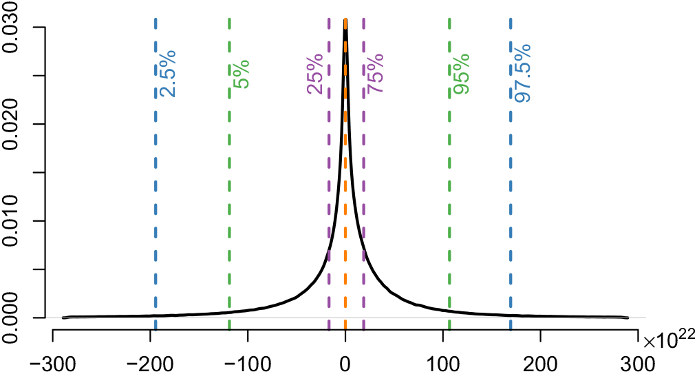
Figure A.1. (Colour online) Kernel density estimator of the difference between the simulated values of ΔV
2 for the unconditional and the conditional specification of $\widehat{\boldsymbol{\theta}}^{\,*}$
(unconditional minus conditional). Position 0 is marked by the orange dashed middle line. The other dashed lines correspond to a chosen set of reference sample quantiles of these differences.
$\widehat{\boldsymbol{\theta}}^{\,*}$
(unconditional minus conditional). Position 0 is marked by the orange dashed middle line. The other dashed lines correspond to a chosen set of reference sample quantiles of these differences.
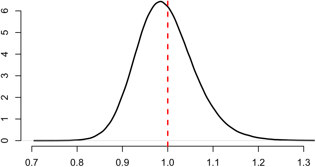
Figure A.2. (Colour online) Kernel density estimator of the ratio between the conditional and the unconditional estimators of the estimation error. Position 1 is marked by the red dashed line.
are computed as well as
 $$x_{k}\,:=\nabla h(\,\widehat{{{{f}}}}^{\,(i)};\,\cal F_0^{(i)})^{\prime} \boldsymbol{\Sigma}_{i,2^k n} \nabla h(\,\widehat{{{{f}}}}^{\,(i)};\,\cal F_0^{(i)})\\\widetilde{x}_{k}\,:=\nabla h(\,\widehat{{{{f}}}}^{\,(i)};\,\cal F_0^{(i)})^{\prime} \boldsymbol{\widetilde{\Sigma}}_{i,2^k n} \nabla h(\,\widehat{{{{f}}}} ^{\,(i)};\,\cal F_0^{(i)})$$
The stopping criterion is
 $$ \frac{|x_k - \widetilde{x}_k|}{\min(|x_k|,|\widetilde{x}_k|)}<0.001$$
Upon stopping, the two independent samples of size 2 k n are merged. Consequently Mi = 2 k+1 n, where k is the smallest number such that the stopping criterion is satisfied.
The results of the simulation study are the following. In Figure A.1, the distribution of the difference between the simulated values of ΔV
2 for the unconditional and the conditional specification of $\widehat{\boldsymbol{\theta}}^{\,*}$
is illustrated. The distribution is leptokurtic, has a slight positive skewness and is approximately centred at zero. The mean and the median of this distribution are small relative the scale of the data (−0.94 × 10²² and 0.28 × 10²², respectively). To quantify the uncertainty in these quantities, 95% bootstrap confidence intervals are computed based on the percentile method, see Efron and Tibshirani (Reference Efron and Tibshirani1994), yielding [ − 1.2, −0.7] × 1022 and [0.2, 0.3] × 1022, respectively, using 105 bootstrap samples. As a matter of fact, none of the bootstrap samples of the mean are above 0 and none of the samples of the median are below 0. This indicates that the unconditional specification is better on average (the mean is negative), but the conditional specification is better more often (the median is positive). The practical relevance of this is, however, questionable since on the relative scale of the data, the mean and median are both approximately zero, indicating that the difference between the two estimators is negligible and that one should therefore focus on the computability of the estimators. In Figure A.2, the ratio between the conditional and the unconditional estimators of the estimation error is shown. From this figure, it is clear that the two estimators are comparable and do not deviate from each other by much.
$\widehat{\boldsymbol{\theta}}^{\,*}$
is illustrated. The distribution is leptokurtic, has a slight positive skewness and is approximately centred at zero. The mean and the median of this distribution are small relative the scale of the data (−0.94 × 10²² and 0.28 × 10²², respectively). To quantify the uncertainty in these quantities, 95% bootstrap confidence intervals are computed based on the percentile method, see Efron and Tibshirani (Reference Efron and Tibshirani1994), yielding [ − 1.2, −0.7] × 1022 and [0.2, 0.3] × 1022, respectively, using 105 bootstrap samples. As a matter of fact, none of the bootstrap samples of the mean are above 0 and none of the samples of the median are below 0. This indicates that the unconditional specification is better on average (the mean is negative), but the conditional specification is better more often (the median is positive). The practical relevance of this is, however, questionable since on the relative scale of the data, the mean and median are both approximately zero, indicating that the difference between the two estimators is negligible and that one should therefore focus on the computability of the estimators. In Figure A.2, the ratio between the conditional and the unconditional estimators of the estimation error is shown. From this figure, it is clear that the two estimators are comparable and do not deviate from each other by much.

Figure A.3. Kernel density estimators of the estimator $\widehat{\alpha}$
of the mean of the first column and the estimator
$\widehat{\alpha}$
of the mean of the first column and the estimator $\widehat{\tau}^2$
of the variance of the first column.
$\widehat{\tau}^2$
of the variance of the first column.
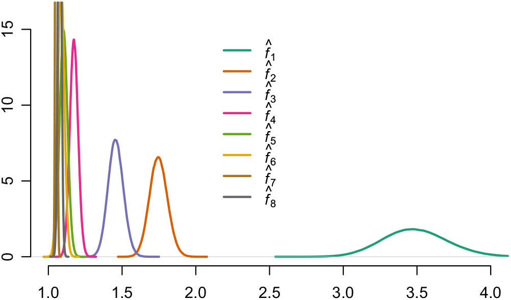
Figure A.4. (Colour online) Kernel density estimators of the estimators of the development factors. Some density curves are cut in order to make it easier to visually discriminate between the development factors centred close to 1.
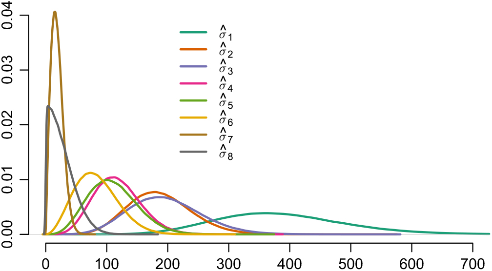
Figure A.5. (Colour online) Kernel density estimators of the square roots of the variance estimators $\widehat{\sigma}_j^2$
.
$\widehat{\sigma}_j^2$
.
The distribution of the difference between the ΔV
2s is heavy tailed, and one is therefore led to question whether this is due to the log-normally distributed error terms. Therefore, the marginal distributions of the components of $\widehat{\boldsymbol{\theta}}$
are illustrated in Figure A.3 (first column parameters), Figure A.4 (development factors) and Figure A.5 (chain ladder variances). The estimators of the intercept of the first column and the development factors are, for all intents and purposes, marginally Gaussian. The variances, however, do have heavier tails (the standard deviations are illustrated in Figure A.5). This can have a large effect on the estimated process variance, and thus in turn on the ΔV
2s.
$\widehat{\boldsymbol{\theta}}$
are illustrated in Figure A.3 (first column parameters), Figure A.4 (development factors) and Figure A.5 (chain ladder variances). The estimators of the intercept of the first column and the development factors are, for all intents and purposes, marginally Gaussian. The variances, however, do have heavier tails (the standard deviations are illustrated in Figure A.5). This can have a large effect on the estimated process variance, and thus in turn on the ΔV
2s.
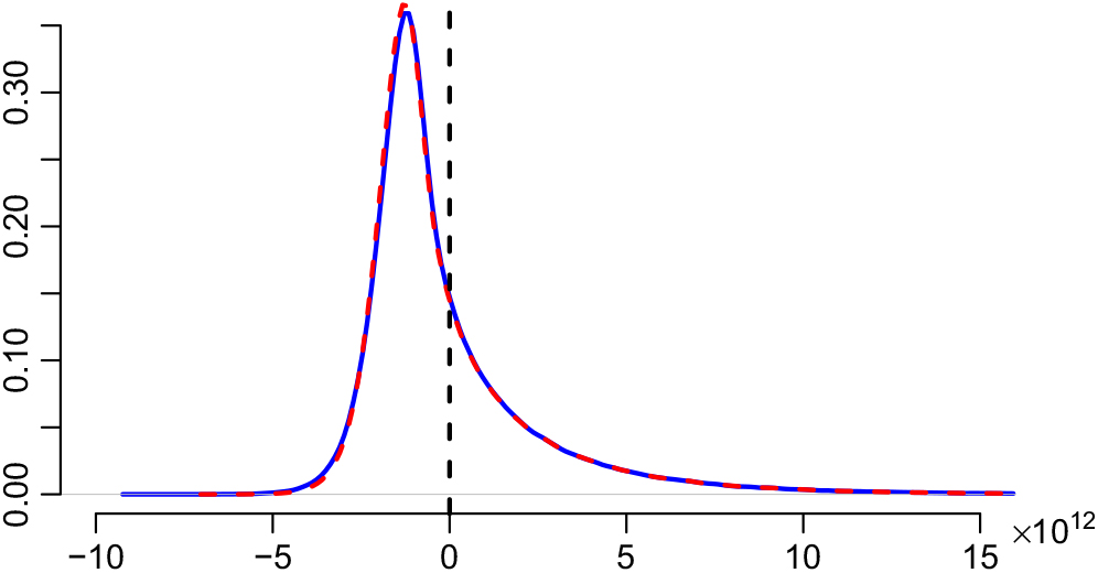
Figure A.6. (Colour online) Kernel density estimators of the true estimation error minus the estimated estimation error based on the conditional (blue solid curve) and the unconditional (red dashed curve) specification of $\widehat{\boldsymbol{\theta}}^{\,*}$
. Position 0 is marked by the black dashed line.
$\widehat{\boldsymbol{\theta}}^{\,*}$
. Position 0 is marked by the black dashed line.
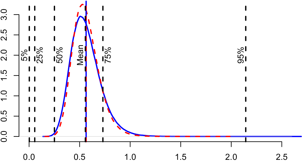
Figure A.7. (Colour online) Kernel density estimator of the ratio of the estimation error and the process variance. The blue solid curve is the density for the estimated version of this ratio based on the conditional specification, and the red dashed curve is for the unconditional specification. The corresponding vertical lines mark the means of the respective distributions. The black dashed vertical lines mark quantiles and mean of the true distribution of this ratio.
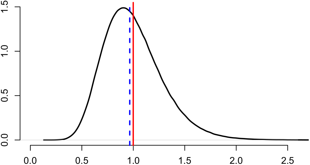
Figure A.8. (Colour online) Kernel density estimator of the ratio between the estimated process variance based on plug-in estimation and the true process variance. The red solid line marks the mean of this ratio and the blue dashed line marks the median.
So far the relative performance of the two estimators has been presented. It is of interest to also investigate the absolute performance. Figure A.6 shows the distributions of the true estimation error minus the estimated ones based on the conditional and unconditional specification of $\widehat{\boldsymbol{\theta}}^{\,*}$
. It is seen that there is a tendency to overestimate the true estimation error, although there is a tail to the right indicating that the estimation error will occasionally be greatly underestimated. The mean estimation error in the simulations is 1.9 × 10¹² and the 95% quantiles of the two above distributions are approximately 5 × 10¹². The estimated estimation error will therefore, in the 95% worst case scenario, be underestimated on the scale of, approximately, 2.5 estimation error means.
$\widehat{\boldsymbol{\theta}}^{\,*}$
. It is seen that there is a tendency to overestimate the true estimation error, although there is a tail to the right indicating that the estimation error will occasionally be greatly underestimated. The mean estimation error in the simulations is 1.9 × 10¹² and the 95% quantiles of the two above distributions are approximately 5 × 10¹². The estimated estimation error will therefore, in the 95% worst case scenario, be underestimated on the scale of, approximately, 2.5 estimation error means.
The practical relevance of estimating the estimation error requires that it is of size comparable to the process variance. Figure A.7 shows the distributions of the estimated estimation errors divided by the estimated process variances, together with dashed black vertical lines indicating some of the quantiles of the distribution of the true estimation error divided by the true process variance. On average, the estimation error is half the size of the process variance, which is also more or less the centre of the distributions of the estimated versions. The median, however, of the true distribution lies approximately around 0.25. Therefore, it is as likely that the estimation error is greater than a quarter of the process variance as that it would be less than a quarter of the process variance.
Finally, to illustrate how plug-in estimation of the process variance performs, Figure A.8 shows the distribution of the ratio between the estimated process variance (based on plug-in) and the true process variance. Both the mean and the median of this distribution lie close to 1, indicating that on average the estimator yields the correct variance and that we are more or less equally likely to overestimate it as to underestimate it. It is also seen that there are extreme cases where the variance is estimated to be either half or double the true variance.


 Open access