


1. Introduction
The magnitude of extreme ocean waves is of interest to engineers and physicists. The former need to design offshore infrastructure and the latter are interested in the fascinating weakly nonlinear processes that lead to the formation of large waves. Of particular interest is whether more large waves (sometimes called freak or rogue waves) occur than would be predicted by linear or second-order theory (see Dysthe, Krogstad & Müller (Reference Dysthe, Krogstad and Müller2008), Onorato et al. (Reference Onorato, Residori, Bortolozzo, Montina and Arecchi2013), Adcock & Taylor (Reference Adcock and Taylor2014) for reviews).
Laboratory experiments are frequently used to investigate the formation of extreme waves. Froude number similarity is generally sufficient for large waves to evolve in the same way in the laboratory and in the ocean. However, one important difference between laboratory and ocean is how the waves are generated. In the ocean, the type of waves we consider in this paper are generated by wind. It is difficult to replicate this experimentally although this has been tried and is an active area of research (e.g. Toffoli et al. Reference Toffoli, Proment, Salman, Monbaliu, Frascoli, Dafilis, Stramignoni, Forza, Manfrin and Onorato2017; Shemer Reference Shemer2019). In most laboratories waves are created using paddles, but this creates a number of issues. Near the paddle evanescent waves form, although these typically decay after a few wavelengths (Schäffer Reference Schäffer1996). It is difficult to suppress ‘error waves’, which are caused by not accurately reproducing the bound harmonics – the low-frequency ‘difference’ term is particularly hard to reproduce with a conventional flap-type paddle and can be problematic in shallower-water experiments (Orszaghova, Borthwick & Taylor Reference Orszaghova, Borthwick and Taylor2012; Whittaker et al. Reference Whittaker, Fitzgerald, Raby, Taylor, Orszaghova and Borthwick2017; Mortimer et al. Reference Mortimer, Raby, Antonini, Greaves and van den Bremer2022). Difficulties in creating the desired statistics in a tank are considered in the recent work of Canard, Ducrozet & Bouscasse (Reference Canard, Ducrozet and Bouscasse2022). A final issue is that paddles will only operate over a finite bandwidth making it difficult to create very broad-banded spectra, and this will often lead to a desired spectrum being modified by setting to zero a small amount of energy above a given cutoff frequency. A similar approach may be taken when initialising numerical simulations. The importance of this cutoff is the subject of the present paper.
In the laboratory (or indeed numerically) it is possible to make sea states that are implausible in the real ocean. For instance, in the laboratory very steep random waves can be generated with a narrow directional spread and small bandwidth, which would be implausible in the ocean as nonlinear energy transfers and wave breaking would cause a downshift of the spectral energy peak and a broadening of the spectrum. In nature it is possible to have part of a spectrum suppressed (e.g. by wave/ice interaction Toffoli et al. (Reference Toffoli, Bennetts, Meylan, Cavaliere, Alberello, Elsnab and Monty2015) or slicks), but waves are expected to naturally rapidly re-establish a high-frequency tail. The high-frequency tail also forms rapidly in experiments if it is not generated by the paddle (Latheef & Swan Reference Latheef and Swan2013) (see also Fadaeiazar et al. Reference Fadaeiazar, Leontini, Onorato, Waseda, Alberello and Toffoli2020). The question addressed herein is whether the nonlinear energy transfers that act to (re-)establish the tail have a significant impact on the number of large waves formed and, therefore, whether or not including the high-frequency tail in the initial conditions is potentially problematic.
Fedele (Reference Fedele2015), building on the work of Janssen (Reference Janssen2003), derived an expression for the evolution of the dynamic kurtosis as the sea state evolves (see also Janssen & Janssen Reference Janssen and Janssen2019), with the dynamic kurtosis being a useful proxy for the number of rogue waves. This predicted that, for directionally spread waves, an initially random sea state that would have zero excess dynamic kurtosis would see an increase in dynamic kurtosis as the waves moved away from the paddle. However, the dynamic kurtosis would then peak before decaying to zero. Fedele's results assumed, amongst other approximations, that the sea state was narrow banded. Applying the results of Fedele's theory to broad-banded spectra can be challenging, as results are dependent on the Benjamin–Feir index squared (e.g. Tang et al. Reference Tang, Xu, Barratt, Bingham, Li, Taylor, van den Bremer and Adcock2020), which itself is dependent on the bandwidth of the spectrum. For broad-banded spectra, bandwidth is difficult to define. However, curtailing the tail of the spectrum (whilst leaving the total energy unaltered) will increase the Benjamin–Feir index, thus implying that a higher peak in excess kurtosis would be expected (and, hence, more rogue waves).
In this paper we consider the impact of removing the high-frequency spectral tail on rogue waves statistics by numerically simulating two seminal experiments, those of Onorato et al. (Reference Onorato2009) and Latheef & Swan (Reference Latheef and Swan2013). We simulate waves using the fully nonlinear potential-flow model OceanWave3D (Engsig-Karup, Bingham & Lindberg Reference Engsig-Karup, Bingham and Lindberg2009). The present study only considers directionally spread waves as, in the open ocean, waves always have a distribution of directions and, thus, directional waves are of most interest. Unidirectional waves have significantly different nonlinear physics (see, for instance, Fedele Reference Fedele2015), and the results described here are unlikely to apply directly to unidirectional scenarios.
2. Methodology
2.1. Cases
We examine two cases based on experimental studies by Onorato et al. (Reference Onorato2009) (O09 hereinafter) and Latheef & Swan (Reference Latheef and Swan2013) (LS13 hereinafter). For each, we perform numerical simulations with and without the high-frequency tail included in the initial conditions. Basic information for both of the experiments are presented in table 1.
Table 1. Dimensions of the laboratory experiments (exp.) and the numerical (num.) domains. Here ST and LT denote short-tail and long-tail cases, respectively.

The experiments of O09 were performed in the MARINTEK directional basin in Norway. In this study we revisit a total of eight measurement locations along the centreline of the basin. In the original study a total of six independent experimental runs with different random realisations were considered, which we combine here. Several authors have numerically simulated the experiments of O09 including the case we choose to repeat (Toffoli et al. Reference Toffoli, Gramstad, Trulsen, Monbaliu, Bitner-Gregersen and Onorato2010; Xiao et al. Reference Xiao, Liu, Wu and Yue2013).
The experiments of LS13 were conducted in the wave basin at Imperial College London. From these experiments, we include the measurements at ‘gauge 2’, which is  $3.1\lambda _0$ from the wavemaker, where $\lambda _0$ is the peak wavelength; which is the gauge analysed in LS13. Their wavemaker had a cutoff (smoothed over a short range) at three times the peak frequency ( $3\omega _0$). The case we choose to simulate from their experiments was also repeated in an alternative basin at MARIN in the Netherlands with consistent results (LS13).
Both studies were based on the JONSWAP spectra for which the bandwidth is controlled using the peak enhancement factor  $\gamma$. In O09 a cosine- $N$ spreading function is used,
 \begin{equation} D_{\rm O09}(\theta)=A_{\rm O09}\cos^{N} (\theta),\end{equation}
where  $\theta$ is the angle deviating from the mean wave direction, $N$ the spreading parameter and $A_{\rm O09}$ a normalising coefficient. In LS13 a normal distribution is used for the spreading function,
 \begin{equation} D_{\rm LS13}(\theta)=\frac{A_{\rm LS13}}{{\varTheta}_1} \exp \left[-\frac{\theta^{2}}{2 {\varTheta}_1^{2}}\right], \end{equation}
where  $\varTheta _1$ is the spreading parameter and $A_{\rm LS13}$ a normalising coefficient. In this study, for O09, we consider the case with $N=840$ based on (2.1), which approximately has an angle of spreading of $\varTheta _1 \approx 2^{\circ }$ based on (2.2).
The initial sea-state parameters considered in each study are given in table 2. The non-dimensional sea-state steepness  $\epsilon =k_{p} H_{s} / 2$, where $k_{p}$ is the peak wavenumber and $H_{s}$ is the significant wave height. For each case, table 2 presents the amount of energy below the cutoff frequency relative to a non-curtailed spectrum in the rightmost column. Note that in all cases the energy has been redistributed after curtailing the spectrum so that the total energy of the initial input spectrum is the same for both short-tail (ST) and long-tail (LT) cases, although we emphasise the effects of the cutoff on the energy are very small. In particular, the zeroth moment of the wave spectrum based on the input spectrum for both LS13 ST and LT cases is 0.00144 m $^2$, of which the energy corresponding to 0.000014 m $^2$ ( $\sim$1 %) is redistributed between the LT and ST cases. For O09 cases, the zeroth moment of the wave spectrum based on the input spectrum is 0.00041 m $^2$ for both ST and LT cases, of which the energy corresponding to 0.000042 m $^2$ ( $\sim$10 %) is redistributed between the LT and ST cases. In all simulations, the sea states are generated by setting the phase of a component to be randomly distributed between $0$ and $2{\rm \pi}$ and drawing the amplitude of each component from a Rayleigh distribution following Tucker, Challenor & Carter (Reference Tucker, Challenor and Carter1984). To make directional sea states, each wave component is assigned a random travelling angle drawn from the specified spreading function (i.e. (2.1) for O09 cases and (2.2) for LS13 cases).
Table 2. Initial sea-state parameters used in this study, where  $\omega _{0}$ is the peak frequency, $k_0$ the peak wavenumber based on the linear dispersion relationship. Water depth, $d$, is presented non-dimensionally. Spreading shows the equivalent spreading angles based on the spreading functions (2.2). The percentage of total energy below the cutoff frequency is given in the rightmost column.

The initial omni-directional spectra are shown in figure 1 where we have used logarithmic axes to highlight the small differences (in terms of energy) between the ST and LT cases. The choice of cutoff frequencies in each case is determined by past studies of these cases. For the O09 simulations, we choose the cutoffs ( $2.4k_0$ for ST and $6k_0$ for LT) to be consistent with Barratt, van den Bremer & Adcock (Reference Barratt, van den Bremer and Adcock2022), who in turn based these values on other numerical simulations in the literature (Toffoli et al. Reference Toffoli, Gramstad, Trulsen, Monbaliu, Bitner-Gregersen and Onorato2010; Xiao et al. Reference Xiao, Liu, Wu and Yue2013). For the LS13 simulations, we choose the cutoff ( $3\omega _0$ for ST) to be consistent with the cutoff in the laboratory experiments of LS13. For the LT case, we do not apply an explicit cutoff but the high tail is, of course, limited by the discretisation of the simulation.

Figure 1. Initial omni-directional frequency variance density spectra for the simulations of the experiments of (a) LS13 and (b) O09.
2.2. Numerical set-up
We solve the standard potential-flow water-wave equations using OceanWave3D (with details given in Appendix A and in Engsig-Karup et al. Reference Engsig-Karup, Bingham and Lindberg2009). The numerical resolutions used are based on the detailed examination of the numerical behaviour and convergence of this code in Barratt, Bingham & Adcock (Reference Barratt, Bingham and Adcock2020). Thus, for the LS13 cases, we use a spatial resolution of 0.113 m (approximately 34 nodes per peak wavelength) and, for the O09 cases, we use a spatial resolution of 0.068 m (approximately 23 nodes per peak wavelength). Eight clustered nodes are used vertically in the water column. The total simulation time is 1800 s with a time step of 0.02 s (80 per peak period). Wave breaking is simulated using a local smoothing filter, which is turned on when the vertical Lagrangian acceleration on the free surface is greater than 0.4  $g$, where $g$ is the gravitational acceleration constant. This local smoothing filter will remove a small amount of energy from the breaking crests until the vertical particle acceleration is below the threshold.
We create waves at one side of the basin using a double relaxation zone to absorb any reflected waves. Waves are absorbed at the far end of the domain using relaxation zones. This mirrors the set-up of the experiments we are comparing against. The width of the absorbing zone in our numerical tank is  $5.26\lambda _0$, where $\lambda _0$ is the peak wavelength. Two additional relaxation zones are implemented at both side walls. These relaxation zones are configured to damp out the velocity component in the transverse direction, which minimises unwanted artefacts from the side-wall reflection. The linear wave generation method is adapted in our numerical scheme, which implies there is no second-order correction for the bound harmonics of the input signal (see details in the introduction and in Schäffer Reference Schäffer1996). The linear wave generation method is also used in the O09 experiment and it is unclear about the wave generation mechanisms used for LS13. For numerical simulations, initiating a simulation with exactly the same content as in a developed sea state is also difficult. Aside from effects from wind input and breaking that might be present, there are a number of nonlinear phenomena present. There will obviously be bound waves that are significant around large waves. There will also be amplification of short waves and crests (and suppression at troughs) due to long/short wave interaction (Longuet-Higgins & Stewart Reference Longuet-Higgins and Stewart1960) as well as there being a cascade of energy from longer to shorter wavelengths. Capturing all of these in directional simulations would be a substantial challenge. We note that the Creamer transform (Creamer et al. Reference Creamer, Henyey, Schult and Wright1989) would capture much for unidirectional waves.
Numerical set-up parameters are given in table 1. We use a number of different lengths in the  $x$ direction for computational reasons. Thus, we have more simulations of the first part of the domain and, hence, more data points and smaller confidence intervals in this part of the domain.
3. Results
3.1. Crest statistics
We start by analysing crest statistics. To reduce statistical uncertainty, we use data from multiple locations at  $90^{\circ }$ to the mean wave direction. For the LS13 cases, we use two measurement locations in the $y$ direction separated by 11.72 m $(3.03 \lambda _0)$. For the O09 cases, we use three measurement locations in the $y$ direction separated by 3.42 m $(2.20\lambda _0)$. These points are far enough apart that there is negligible correlation, and this helps the clarity of the results. We present data normalised using the initial conditions measured at $x=0$.
3.1.1. O09
First, we examine the O09 case. Figure 2 compares the exceedance probabilities of crests at four locations along the length ( $x$ direction) from the experiments and for the ST and LT simulations. Also shown for comparison is the commonly used distribution by Forristall (Reference Forristall2000), which is based on second-order theory. The shaded regions correspond to 90 % confidence intervals for the simulations based on the bootstrap method (Efron & Tibshirani Reference Efron and Tibshirani1994). To examine the crest statistics of O09 further, we also consider crest exceedance probabilities as a function of the distance along the length of the basin ( $x$). We choose to analyse the amplitude of crests with a $10^{-3}$ probability of exceedance (i.e. the 1/1000 wave). This threshold is a trade-off between statistical robustness and capturing the tail behaviour. However, the conclusions do not change if we use alternative values. For O09, these data are presented in figure 3.

Figure 2. For O09, crest exceedance probabilities at four different distances from the paddle (locations of gauges in the experiments of O09): (a)  $x=3.1\lambda _0$, (b) $x=6.3\lambda _0$, (c) $x=12.6\lambda _0$, (d) $x=22.3\lambda _0$ for ST and LT simulations. The shaded regions correspond to 90 % confidence intervals for the simulations based on the bootstrap method. The results O09 $_{\rm ST}$ and O09 $_{\rm LT}$ are obtained through fully nonlinear potential-flow simulations. Also shown are the experimental results from O09.

Figure 3. For O09, wave crest amplitude at the  $10^{-3}$ crest exceedance probability level for ST and LT simulations. The shaded regions correspond to 90 % confidence intervals for the simulations based on the bootstrap method. Also shown are the experimental results from O09. A zero-phase shift Fourier filter is applied to smooth out short-term fluctuations within the length scale of $0.4\lambda _0$.
The same general trends occur in experiments and both simulations. All predict more large waves than predicted by Forristall's second-order theory, which is not unexpected for this steep and narrow-banded case. As is evident from figure 3 for small  $x/\lambda _0$, in the simulations there is a spike in the number of large waves near the inlet that is presumed to be due to ‘error waves’ in the wave generation. Away from the inlet the number of large waves observed increases for a distance of approximately $12\lambda _0$ before falling again. The wave crests for the ST case are generally higher than for the LT case, and this difference is mostly statistically significant, especially for the first $12\lambda _0$. It is not known exactly what frequency cutoff was applied in the experiments so it is not possible to say whether the experiments support one or other of our simulations. However, although both simulations appear to overestimate slightly the numbers of large waves, they do provide a useful confirmation of the validity of our simulations. The key result for the present paper is the dependence of the simulation on the high-frequency cutoff selected. Whilst there is the expected statistical variation, the short-tailed initial spectrum clearly produces more large crests than the long-tailed spectrum, although these appear to get closer as one moves down the basin.
3.1.2. LS13
Second, we analyse the crest statistics for the LS13 case. Figure 4 shows the crest exceedance probability at four locations along the length of the basin (noting that experimental data are only available at the second location:  $x = 1.075\lambda _0$). We again consider the amplitude of the crests at the $10^{-3}$ probability level in figure 5.

Figure 4. For LS13, crest exceedance probabilities at four different distances from the paddle: (a)  $x=0.3\lambda _0$, (b) $x=1.075\lambda _0$ (location of the gauge in the experiments of LS13), (c) $x=1.76\lambda _0$, (d) $x=16.1\lambda _0$. The shaded regions correspond to 90 % confidence intervals for the simulations based on the bootstrap method. The results LS13 $_{\rm ST}$ and LS13 $_{\rm LT}$ are obtained through fully nonlinear potential-flow simulations. Also shown are the experimental results from LS13.

Figure 5. For LS13, wave crest amplitude at the  $10^{-3}$ crest exceedance probability level for ST and LT simulations. The shaded regions correspond to 90 % confidence intervals for the simulations based on the bootstrap method. Also shown are the experimental measurements from LS13. A zero-phase shift Fourier filter is applied to smooth out short-term fluctuations within the length scale of $0.4\lambda _0$.
We again observe a rapid increase in the number of large waves close to where the waves are generated that dies away by  $0.5\lambda _0$. We also see that the number of extreme crests is lower in the LS13 compared with O09. This is expected as the LS13 is less steep and has a broader bandwidth. In both simulations there appears to be an increase in the number of extreme crests observed as one moves down the tank. Possibly, this is the same effect as observed in the O09 case up to $12\lambda _0$, but the non-dimensionally shorter domain does not show a peak (where non-dimensional length is based on the scaling of Fedele (Reference Fedele2015); see § 3.2).
However, it is clear that there are substantial and statistically significant differences between the probability of large waves when the tail is and is not included in the wavemaker signal. When the tail is included in the initial conditions, the distribution remains close to the distribution of Forristall (Reference Forristall2000). However, there is a clear departure from this distribution when the tail is omitted. It can further be seen that there is better agreement between the experiments of LS13 and the numerical simulations with the short tail compared with the long tail.
We do not present results for wave height distribution in the present paper as we have already considered two metrics for the free surface distribution. However, we note that wave height variations are consistent with the rest of the results presented in the paper.
3.2. Kurtosis of the free surface and comparison with Fedele (Reference Fedele2015)
Moving on from crest statistics, we now analyse our results using the common proxy for rogue wave density, namely the excess kurtosis of the free surface (see Mori & Janssen Reference Mori and Janssen2006). The excess kurtosis  $C_4$ is given by the kurtosis of the free surface minus 3, as a linear Gaussian surface elevation would correspond to a kurtosis of 3. The excess kurtosis $C_4$ is comprised of dynamic $(C_4^d)$ and bound $(C_4^b)$ contributions, such that $C_4=C_4^d+C_4^b$, where the dynamic contribution accounts for the build-up of phase correlation and the bound contribution accounts for the presence of bound harmonics.
A number of other authors have used O09 as the basis for numerical simulations and have studied the kurtosis evolution. Toffoli et al. (Reference Toffoli, Gramstad, Trulsen, Monbaliu, Bitner-Gregersen and Onorato2010) and Xiao et al. (Reference Xiao, Liu, Wu and Yue2013) performed both modified nonlinear Schrödinger (MNLS) equation and fully nonlinear simulations to examine the evolution of the sea state. Furthermore, Barratt et al. (Reference Barratt, van den Bremer and Adcock2022) conducted only MNLS simulations but looked explicitly at the impact of the spectral cutoff. We refer the reader to the original papers for full details of their numerical methods. However, pertinent to the current studies, the high-wavenumber cutoffs for the different simulations are given in table 3. No cutoff is documented as being applied in the original experiments of O09, although we presume the physical limitations of the paddles meant that a full high-frequency tail could not be created.
Table 3. Wavenumber cutoffs used in the literature to simulate O09.

3.2.1. O09
The evolution of kurtosis for our simulations is shown in figure 6, comparing to the experimental results of O09 and the simulations detailed in table 3. We have plotted the data on different subfigures depending on whether the spectrum was severely curtailed to improve clarity, showing the ST cases in panel (a) and the LT cases in panel (b). Experiments are shown in both. In some cases in the literature (see table 3) wave fields that are homogeneous in space are evolved in time. In these cases space/time mapping is done using the group velocity (see, for instance, Chabchoub & Grimshaw Reference Chabchoub and Grimshaw2016), which is strictly only valid in the narrow-banded limit. The  $x$ axes in figure 6 show the corresponding spatial $x/\lambda _0$ or temporal $t/(2T_0)$ parameters with kurtosis shown on the $y$ axis (including the contribution of bound harmonics). Here, $\lambda _0$ and $T_0$ represent the peak wavelength and wave period, respectively.

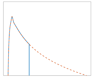
Figure 6. Kurtosis evolution for  $\text {O09}_{\text {ST}}$ (red line) and $\text {O09}_{\text {LT}}$ (blue line) compared against other studies. (a) The cases with truncated tails; these cases are Xiao et al. MNLS ( $-\!-\!-$), Toffoli et al. MNLS ( $\circ$) and Barratt et al. MNLS ST case (red $-\!-\!-$). (b) The cases without truncated tails; these cases are Xiao et al. HOS (——), Toffoli et al. HOS ( $\times$) and Barratt et al. MNLS LT case (blue $-\!-\!-$). The shaded bands represent 95 % confidence intervals based on the standard deviation of different realisations. The coloured dash line indicates the peak kurtosis value for $\text {O09}_{\text {ST}}$ and $\text {O09}_{\text {LT}}$, respectively.
All the results show the same general trends with the kurtosis peaking at approximately  $15\lambda _0$ (or equivalent in time) away from the generation zone. All simulations overestimate the kurtosis relative to the experiment except the LT simulation of Barratt et al. (Reference Barratt, van den Bremer and Adcock2022) beyond $20\lambda _0$.
The key result for the present paper is that we again observe a difference between the short- and long-tailed simulations, with the curtailed spectrum producing more extreme waves than the case with the spectrum cutoff at  $6k_0$. However, whilst this difference is significant, the difference is much less than Barratt et al. (Reference Barratt, van den Bremer and Adcock2022) found when carrying out MNLS simulations using the same parameters. Important differences between the fully nonlinear simulations and the MNLS simulations of Barratt et al. (Reference Barratt, van den Bremer and Adcock2022) are the different evolution models, the need to explicitly calculate bound harmonics in the MNLS, the lack of wave breaking in the MNLS and the work of Barratt et al. (Reference Barratt, van den Bremer and Adcock2022) is homogenous in space and the other simulations listed in Table 3 are in time. However, despite these differences in the modelling, the discrepancy between the two results is significant. Due to the modelling differences it is harder to say anything definitive about the simulations of Toffoli et al. (Reference Toffoli, Gramstad, Trulsen, Monbaliu, Bitner-Gregersen and Onorato2010) and Xiao et al. (Reference Xiao, Liu, Wu and Yue2013) as regards cutoff. For example, a low-pass filter is applied in the higher-order spectral method (HOSM) to model the energy dissipation due to wave breaking in Xiao et al. (Reference Xiao, Liu, Wu and Yue2013), which is absent for HOSM implemented by Toffoli et al. (Reference Toffoli, Gramstad, Trulsen, Monbaliu, Bitner-Gregersen and Onorato2010). This could lead to kurtosis differences shown in figure 6(b). However, their results are generally supportive of the conclusion that curtailing the spectrum increases the number of extreme waves.
Fedele (Reference Fedele2015) derived analytical predictions for the evolution of the kurtosis. Applying this requires the evaluation of the spectral bandwidth. Multiple definitions exist in the literature and the results are sensitive to which bandwidth definition is used. Fedele (Reference Fedele2015) uses the ‘half-width’ parameter that gives identical results for both the truncated tail and the full tail simulations. Using this estimate of bandwidth we get a value of the aspect ratio of the initial spectrum,  $R$, of 0.031, where $R$ is a measure of short crestedness of the dominant waves (see Fedele (Reference Fedele2015) for details). Given that this predicts identical evolution regardless of cutoff, we instead calculate bandwidths using
 \begin{equation} \nu(t)=\frac{1}{\sqrt{\rm \pi}\,Q_0},\end{equation}
where  $Q_0$ is the peakedness parameter used to calculate the Benjamin–Feir index by Serio et al. (Reference Serio, Onorato, Osborne and Janssen2005). Using this parameter gives values of $R=0.045$ for $\text {O09}_{\text {LT}}$ and $R=0.065$ for $\text {O09}_{\text {ST}}$. Figure 7 presents the predicted evolution of excess kurtosis in O09 based on these differing bandwidth estimates along with our numerical results. We note that the bound-wave contribution to the excess kurtosis is also included for both simulated results and the theoretical curves presented in this study (the theoretical curves are obtained following (1.3) for bound harmonics and (2.16) for dynamic excess kurtosis in Fedele Reference Fedele2015).

Figure 7. Excess kurtosis evolution for case  $\text {O09}_{\text {ST}}$ (red line) and case $\text {O09}_{\text {LT}}$ (blue line) compared against the solution of Fedele (Reference Fedele2015) based on the initial wave spectrum at $x=0\lambda _0$ for both cases. The shaded bands represent 95 % confidence intervals based on the standard deviation of different realisations.
In general, agreement between theory and experiment is good. The overall shape and the (non-dimensional) location of maximum kurtosis is predicted well for both cases. The initial evolution is generally well predicted, particularly for the narrower banded ST spectrum. However, the magnitude of kurtosis downstream of the peak appears to reduce faster than predicted by theory. The evolution of excess kurtosis presented herein agrees well with previous numerical simulations reported by Barratt et al. (Reference Barratt, van den Bremer and Adcock2022), where similar faster reduction of kurtosis is also observed towards the end of the basin. We do not think that this deviation from the theory is primarily caused by the local smoothing filter utilised in our numerical model to simulate breaking, as the MNLS equation simulations of Barratt et al. (Reference Barratt, van den Bremer and Adcock2022) do not have such a dissipation but show a similar trend.
3.2.2. LS13
We now turn to the kurtosis evolution for the LS13 case. This is significantly broader banded than O09. As we have no other simulations or experiments to compare with, we simply consider the comparison with the theory developed by Fedele (Reference Fedele2015). Using the bandwidth estimated by Serio et al. (Reference Serio, Onorato, Osborne and Janssen2005), a much smaller excess kurtosis is predicted, and the evolution of both LT and ST cases are nearly identical. Figure 8 presents the predicted evolution of kurtosis. We plot the kurtosis including the contribution from the bound harmonics (and include these in the theoretical lines as well).

Figure 8. Evolution of kurtosis for case  $\text {LS13}_{\text {ST}}$ and case $\text {LS13}_{\text {ST}}$ compared with the predictions of Fedele (Reference Fedele2015) based on the initial wave spectrum at $x=0$ for both cases. The shaded bands represent 95 % confidence intervals based on the standard deviation of different realisations.
As with the results for exceedance probabilities, there is a clear difference between the kurtosis of the two LS13 simulations. This is not predicted by the theory of Fedele (Reference Fedele2015). The initial oscillation, seen in crest exceedance plots, is again present. Following this transience, the kurtosis changes little over the length of the simulation. There may be a small increase with distance, consistent with the theoretical prediction. Whilst the theory does seem to agree well for  $\text {LS13}_{\text {ST}}$, $\text {LS13}_{\text {LT}}$ is over-predicted. However, for this case, all the values of kurtosis are small (consistent with other studies such as Klahn, Madsen & Fuhrman Reference Klahn, Madsen and Fuhrman2021b).
3.3. Spectral changes
We examine how parameters that characterise the (spectrum of the) sea state evolve. We look at two properties. First, we examine the significant steepness  $\xi$, defined as
 \begin{equation} \xi= \frac{2{\rm \pi} H_s}{g T_m^2},\end{equation}
where  $H_s$ is the significant wave height, which corresponds to four times the standard deviation of the surface elevation, and $T_m$ is the mean wave period, which is given by
 \begin{equation} T_m= \sqrt{m_0/m_2},\end{equation}
where  $m_0$ and $m_2$ are the zeroth and second moment of the omni-directional spectrum $S(f)$. We also consider the bandwidth, $\nu$, as defined in (3.1). Figures 9 and 10 present these for O09 and LS13, respectively.

Figure 9. (a) Spatial evolution of significant steepness  $\xi$ for $\text {O09}_{\text {ST}}$, $\text {O09}_{\text {LT}}$ and experimental results presented in O09. The results are normalised by the initial value of $\text {O09}_{\text {LT}}$. (b) Spatial evolution of spectral bandwidth parameter $\nu$ for $\text {O09}_{\text {ST}}$, $\text {O09}_{\text {LT}}$ and experimental results presented in O09. The results are normalised by the initial value of $\text {O09}_{\text {LT}}$.

Figure 10. (a) Spatial evolution of significant steepness  $\xi$ for both $\text {LS13}_{\text {ST}}$ and $\text {LS13}_{\text {LT}}$ cases normalised by the initial value of $\text {LS13}_{\text {LT}}$. (b) Spatial evolution of spectral bandwidth parameter $\nu$ for both $\text {LS13}_{\text {ST}}$ and $\text {LS13}_{\text {LT}}$ cases normalised by the initial value of $\text {LS13}_{\text {LT}}$.
The changes in both steepness and bandwidth are pronounced for the more nonlinear O09 case. Indeed, the changes suggest that (even for the LT case) the spectrum is out of equilibrium leading to a downshift in the spectral peak and broadening of the spectrum. For this case, the experiments are in good agreement with the long-tailed simulation over the first part of the tank (roughly up to the peak in kurtosis), but in the second half the numerics see greater changes than the experiments. Changes to the sea-state parameters are much smaller for the LS13 case although there appears to be a modest increase in bandwidth and a spectral downshift particularly early in the simulation. We also observe a similar decreasing trend in wave steepness, especially for the experiments and numerical results of the more nonlinear O09 case. This decrease in space is likely attributed to the energy dissipation due to wave breaking during the experiment and the local breaking filter in the numerical simulations (see details in § 2.2).
The key result for the purpose of this paper is a comparison of the long- and short-tailed simulations. The main differences here are at the start of the simulation particularly for O09 where ST and LT have opposite trends over the first few wavelengths for both bandwidth and steepness. Apart from this, the evolution is similar although it is noticeable that in all results there are differences at the end of the basin between ST and LT simulations. This shows that one cannot just assume that there are some rapid changes as the full spectral tail grows and for the evolution to then be the same – this conclusion is of course consistent with the results for extreme waves discussed above.
3.4. Application to wave loading of a surface-piercing column
Studying the statistics of wave kinematics directly is difficult. Furthermore, the important practical question asked in this paper is whether loads measured experimentally are dependent on the high-frequency cutoff used. We therefore follow Paulsen et al. (Reference Paulsen, Bredmose, Bingham and Jacobsen2014), Klahn, Madsen & Fuhrman (Reference Klahn, Madsen and Fuhrman2021a) and consider loads on an idealised structure using a simple loading model. In this case we choose to use the drag part of Morison's equations to predict the overturning moment around the sea bed of a uniform structure. Thus, the load is given by
 \begin{equation} F(z,x,t)=\rho \frac{D}{2} C_D u |u|,\end{equation}
where  $F(z,x,t)$ is force per unit length on a fixed vertical cylinder with a nominal diameter of $D$ located at a specific spatial location $(x,z)$, and $z$ is the vertical coordinate. In (3.4), $\rho$ is the water density, $C_D$ is the drag coefficient and $u$ is the horizontal velocity at the corresponding time and space. Note that OceanWave3D explicitly solves for the wave kinematics, and so we use the velocity directly from the simulations. The force is integrated over the column to give the overturning moment around the bed.
We analyse the output time series by analysing the moment magnitude that is exceeded for  $0.5\,\%$ of the simulation, which we refer to as $M$. Again, the choice of $0.5\,\%$ is a trade-off between statistical robustness and analysing the extremes we are primarily interested in. Figures 11 and 12 show how this metric evolves along the length of the numerical tank for O09 and LS13, respectively. We observe the same fundamental trends in the evolution of moment as we do for surface properties. The ST simulations generate a substantially higher overturning moment compared with the long-tailed simulations although these are significantly closer for the LS13 case. This strongly implies that there are more extreme kinematics in the simulations with a short-tailed spectrum.

Figure 11. For O09, the overturning moment magnitude exceeded 0.5 % of the total simulation time normalised by its initial value (at  $x=0$) for $\text {O09}_{\text {LT}}$. The shaded bands represent 90 % confidence intervals based on the bootstrap method.

Figure 12. For LS13, the overturning moment magnitude exceeded 0.5 % of the total simulation time normalised by its initial value (at  $x=0$) for $\text {LS13}_{\text {LT}}$. The shaded bands represent 90 % confidence intervals.
4. Discussion
Our results suggest that minor differences in the initial spectrum of random wave simulations or experiments can lead to a significant change to the number of rogue waves observed and to loads predicted on structures placed in the waves. Our simulations appear to be consistent with other simulations carried out in the literature even if these were not explicitly looking at the phenomenon. This result has a potentially significant impact for random wave investigations (both looking directly at the waves but also for offshore model testing). This is particularly true for laboratory tests where physical limitations of the paddles are a constraint on the waves that can be generated. However, we highlight that although we have strong evidence from simulations here, we have not been able to do laboratory experiments to investigate this. To do so would require redesigning the wavemaker and would be a major undertaking. This paper provides evidence that there is a practical problem here and we think justifies more work to both explain the results and find a way of avoiding this effect in experiments.
The findings in this paper came as a surprise to the authors. The changes to the initial spectra are minor (particularly for the LS13 case) yet produce significantly different results. This said, the results are consistent with the study of Barratt et al. (Reference Barratt, Bingham, Taylor, Van Den Bremer and Adcock2021). In Barratt et al. (Reference Barratt, Bingham, Taylor, Van Den Bremer and Adcock2021) deterministic wave groups were shown to evolve very differently with and without the high-frequency tail. The deterministic study of Barratt et al. (Reference Barratt, Bingham, Taylor, Van Den Bremer and Adcock2021) provides a basis for the results presented here as some of the physics may be clearer for deterministic groups than in random seas.
The physical mechanism at play here is not fully understood. However, the ideas of spectral equilibrium appear to be important, particularly the equilibrium of the spectral tail, which various authors have considered in different contexts (Waseda, Toba & Tulin Reference Waseda, Toba and Tulin2001; Annenkov & Shrira Reference Annenkov and Shrira2006; Viotti & Dias Reference Viotti and Dias2014; Trulsen Reference Trulsen2018). There is clearly an interplay between the nonlinear physics trying to establish a smooth tail in which the components are in equilibrium and the creation of correlation between wave components, leading to an abnormal number of large waves.
Some aspects of the physics identified in this paper are caught by the narrow-banded theory of Fedele (Reference Fedele2015), but it cannot capture all the dynamics of realistically broad-banded seas despite being a useful starting point.
5. Conclusions
We have simulated two classic random wave experiments from the literature, namely Onorato et al. (Reference Onorato2009) and Latheef & Swan (Reference Latheef and Swan2013), using a fully nonlinear potential-flow solver. We have examined the significance of making minor modifications to our initial conditions, suppressing the high-frequency content in the initial conditions of some of the simulations as is routine in the literature and a practical necessity in a laboratory experiment. Despite these changes being small, they lead to significant differences in the number of large waves and persist for tens of wavelengths after the waves are generated. Furthermore, when the full spectral tail is used in the initial conditions there is minimal extra elevation beyond that expected by second-order theory, consistent with work such as Fedele et al. (Reference Fedele, Brennan, Ponce De León, Dudley and Dias2016), for the LS13 sea state, which has parameters that are plausible in the open ocean.
Our results suggest that care is needed in initialising simulations or experiments where the aim is to reproduce open-ocean conditions. Except in exceptional circumstances, in the open ocean a fully developed spectral tail will be present and the spectrum will be, at least roughly, in equilibrium. The problem identified herein is a particular problem for experimental facilities where it is difficult to create a broad frequency range with a conventional paddle, and physical limitations mean that tanks cannot be hundreds of wavelengths long to negate this issue.
Acknowledgements
The authors thank M. Christou (Imperial College London) for several insightful conversations about this work and A. Toffoli (University of Melbourne) and M. Onorato (Università di Torino) for sharing their data. T.S.V.D.B. acknowledges a Royal Academy of Engineering Research Fellowship.
Funding
T.T. was funded by an COVID extension to EPSRC/NERC grant EP/R007632/1 and is now funded by EPSRC grant EP/V050079/1.
This research was funded in whole or in part by [EPSRC] [EP/V050079/1]. For the purpose of open access, the author has applied a CC BY public copyright licence to any Author Accepted Manuscript (AAM) version arising from this submission.
Declaration of interests
The authors report no conflict of interest.
Appendix A. Governing equations of OceanWave3D
OceanWave3D model is based on the flexible-order finite difference discretisations to determine the exact potential-flow solutions (Engsig-Karup et al. Reference Engsig-Karup, Bingham and Lindberg2009). OceanWave3D model can also generate the internal kinematics without extra computation steps since the potential-flow equations are solved within the fluid domain. We consider the fluid velocity in all three directions (i.e. x, y, z), which are noted as u, v and w respectively. These velocity components can be calculated by the gradient of the velocity potential  $\phi (x,y,z,t)$,
 \begin{equation} u,v,w=(\boldsymbol{\nabla}\phi,\partial_z\phi), \end{equation}
in which  $\boldsymbol {\nabla }=(\partial _x,\partial _y)$ is the horizontal gradient operator. Following the equation established by Zakharov (Reference Zakharov1968), the kinematic and dynamic free surface boundary conditions are expressed in terms of velocity potential in (A2) and (A3), which can be formulated by using the chain rule on the nonlinear version of the Bernoulli equation as well as the nonlinear kinematic boundary condition,
 $$\begin{gather} \partial_t\eta={-}\boldsymbol{\nabla}\eta\boldsymbol{\cdot} \boldsymbol{\nabla}\tilde{\phi}+\tilde{w}(1+\boldsymbol{\nabla} \eta\boldsymbol{\cdot}\boldsymbol{\nabla}\eta), \end{gather}$$
 $$\begin{gather}\partial_t\tilde{\phi}={-}g\eta-\tfrac{1}{2}(\boldsymbol{\nabla} {\tilde{\phi}}\boldsymbol{\cdot}\boldsymbol{\nabla}{\tilde{\phi}}- \tilde{w}^2(1+\boldsymbol{\nabla}{\eta}\boldsymbol{\cdot} \boldsymbol{\nabla}{\eta})), \end{gather}$$
in which  $\tilde {\phi }=\phi (x,y,\eta,t)$ is the velocity potential at the free surface ( $z=\eta$), and $\tilde {w}=\partial _z\phi |_{z=\eta }$ is the vertical velocity at the free surface. To obtain the exact value of the vertical velocity in a specific time, the Laplace equation in the fluid is solved, along with the kinematic and dynamic boundary conditions.
This numerical scheme is embedded with a classical four-stage, fourth-order Runge–Kutta scheme for calculating the time integration of the free surface. In terms of the spatial discretisation, OceanWave3D defines a meshed grid point along the horizontal  $xy$ axes, and the free surface field $\eta$ and the velocity potential field $\phi$ are to be evolved at all grid points. All the spatial derivatives of the free surface field are calculated through the discrete counterparts according to the finite difference scheme with nonlinear terms expressed explicitly by direct product approximations at the collocation points. For the treatment of numerical boundary conditions of the domain, Neumann boundary conditions of the normal component of velocity are satisfied.
To solve the transformed Laplace problem, vertical grid points are defined below every horizontal free surface grid point with spacing described following the (non-conformal)  $sigma$-coordinate transformation,
 \begin{equation} \sigma \equiv \frac{z+h(\boldsymbol{x})}{\eta(\boldsymbol{x}, t)+h(\boldsymbol{x})}, \end{equation}
where  $z$ is the vertical coordinate of the grid point, $\boldsymbol {x}$ is the horizontal positioning vector and $h$ specifies the water depth from the still water level.
This structured grid configuration allows direct implementation of finite difference schemes to obtain first and second derivatives with flexible orders (in the present paper a sixth order in the finite difference scheme is adopted following Barratt et al. Reference Barratt, van den Bremer and Adcock2022). This can be achieved by a standard method using Taylor series expansion on all the grid points (Engsig-Karup et al. Reference Engsig-Karup, Bingham and Lindberg2009).


 Open access