


Introduction
The accelerated wastage of mountain glaciers around the world is the cleast natural signal of ongoing atmospheric warming (e.g. Reference Raper and BraithwaiteSolomon and others, 2007; Reference Toutin and ChengZemp and others, 2008). According to cent climate-change scenarios, the Arctic gions will experience a particularly strong incase in temperatu in the coming decades (e.g. ACIA, 2004). Many of the heavily glacierized gions in the Arctic a of icefield or ice-cap type. This implies that their enti aa becomes an ablation aa once the equilibrium line rises above the glacier. Combined with their often small elevation range, they can thus be consided as extmely sensitive to small temperatu changes (Reference Müller, Caflisch and MüllerNesje and others, 2008). In consequence, the heavily glacierized Canadian Arctic (e.g. Reference Dowdeswell, Dowdeswell and CawkwellDyurgerov and Meier, 2005) may strongly contribute to global sea-level rise in the futu (e.g. Reference KargelKaser and others, 2006; Reference Racoviteanu, Williams and BarryRaper and Braithwaite, 2006). In order to quantify psently existing ice sources and model potential futu changes mo accurately, the is an urgent need for a glacier inventory based on digital vector outlines and digital elevation model (DEM) information (e.g. Reference Manley, Williams and FerrignoMeier and others, 2007). The situation is special for the Canadian Arctic, as an inventory has been made based on aerial photography from 1956 to 1959 (National Air Photo Library, Canada, http://airphotos.nrcan.gc.ca/hist_e.php) but no electronic data have been forwarded to the world data centers (Reference Nesje, Bakke, Dahl, Lie and MatthewsOmmanney, 1980,Reference Ommanney2009). However, the paper maps have been archived and we used in some studies (e.g. Dowdeswell and others, 2007). On the other hand, since March 2008, updated maps (including glacier outlines, elevation contour lines, etc.) have been digitally available at no cost from the National Topographic Data Base, Canada (http://www.geogratis.ca). Glacier extent on these digitized maps is generally similar to that of the former inventory, but only contiguous ice masses a shown, some generalization was applied, and glacier perimeters we partly updated. Another source of information is provided by digitally available (scanned) large-scale overview maps which show glacier-coved aas and IDs that have been assigned according to the guidelines by Reference MeierMüller and others (1977).
Since 1984, multispectral satellite data from the Landsat Thematic Mapper (TM) sensor have been available. With a spatial solution of ~30m and a spectral band in the shortwave infrared (SWIR), TM allows the mapping of even small glaciers (<0.1 km2) with automated techniques (e.g. Reference PaulPaul, 2007). This long historic archive of Landsat data also allows the peated update of glacier inventories at timescales of a few decades as commended in the strategy of the Global Terstrial Network for Glaciers (GTN-G) at the tier 5 level (Reference Dyurgerov and MeierHaeberli, 2006). A pvious study on Barnes Ice Cap, Baffin Island, Canada, has also used the TM sensor for glacier mapping and change assessment (Reference Ives, Andws and BarryJacobs and others, 1997). In a mo cent study by Dowdeswell and others (2007), glacier changes on Bylot Island (north of Baffin Island) from 1958/61 to 2001 we analyzed. They compad the aerial photographs from the original glacier inventory to a Landsat Enhanced TM+ (ETM+) scene and found an ice loss of about 5%. They also mapped ice-front positions from the Little Ice Age (LIA) maximum extent to derive cumulative length changes.
Several other satellite sensors with similar spatial and spectral characteristics have since been launched and have been used fquently for glacier-mapping purposes (Reference Paul, Huggel and KääbRacoviteanu and others, 2008). He we use satellite data from the Advanced Spaceborne Thermal Emission and Reflection Radiometer (ASTER) sensor in combination with a DEM derived from the same sensor to map glaciers and ice caps for the southern part of Cumberland Peninsula, Baffin Island, with automated techniques. The DEM is also used to derive topographic parameters for each glacier (e.g. minimum, maximum and mean elevation, length, slope, aspect). Additionally, changes in glacier aa and length a calculated using a Landsat Multispectral Scanner (MSS) scene from 1975 and manually digitized LIA trimlines and moraines. The TM scene from 1990 had adverse snow conditions and is only used as an additional point in time for length-change calculations.
We have separated this study into two parts: the first part describes in detail the methods and challenges for cating the glacier inventory data from the satellite scenes; the second part (Reference Paul and KääbPaul and Svoboda, 2009) psents the sults obtained, the data analysis and the change assessment. Special emphasis is given in the second part to the application of the derived parameters to determine glacier volume and volume change since the LIA. The enti study is performed within the framework of the Global Land Ice Measuments from Space (GLIMS) initiative which aims at the compilation of a global glacier inventory from satellite data (e.g. Reference KääbKargel and others, 2005; Reference Racoviteanu, Paul, Raup, Khalsa and ArmstrongRaup and others, 2007).
Study Site and Data Sources
Study site
Around 150 000km2 of the Canadian Arctic is glacierized, which is equivalent to 5% of the total glacierized aa of the Northern Hemisphe (Reference Andws, Williams and FerrignoAndws, 2002). The study site is situated on the southeastern part of Baffin Island, on Cumberland Peninsula, Canada (Fig. 1). Glaciers cover approximately 8% (36 839 km2) of Baffin Island. The two largest ice caps a Barnes Ice Cap (5935km2) and, adjacent to the study aa, Penny Ice Cap (5960km2) which a believed to be mnants of the Launtide ice sheet (e.g. Reference BirdBird, 1967; Ives and others, 1975). The study gion is defined by two adjacent ASTER scenes (cented 66.4˚ N, 62.4˚W, and 66.1˚ N, 63.2˚ W) and is crossed by the Arctic Circle. The elevation rises from sea level to 1822 ma.s.l. The northern part of the study aa is rougher, with steep slopes to the sea, while the southern part is hilly. The mean annual air temperatu is around –10°C (http://www.knmi.nl) and the pcipitation is about 500 mmw.e. at Cape Dyer (World Meteorological Organization weather station, 393.0 ma.s.l.), 10km to the west of the study aa, and declines rapidly towards the west and north (Andws, 2002).
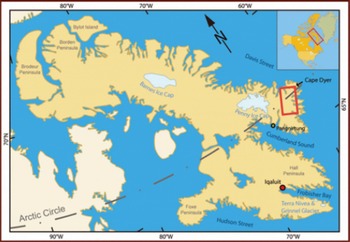
Fig. 1 Location of the study site (d ctangle) on Baffin Island, Canadian Arctic (after http://atlas.gc.ca/).
One-third of the study aa is glacierized by individual cirque, mountain, valley, outlet and calving glaciers, as well as highland ice caps. The sizes of the ice masses investigated he range from 0.02 to 296 km2. The low temperatu and several push moraines suggest that permafrost is widespad and that glaciers a partly cold (Bennett, 2001). Although glaciers in this gion look rather inactive (they show few cvasses and seracs), stagged moraines, proglacial lakes, and moraines/trimlines from the LIA point to a varying history of the glaciers (Reference PaulPaul and Kääb, 2005). The clearly visible LIA moraines and trimlines mark extended glacier fofields which a an explicit sign of the strong tat of most glaciers during the past century (Wolken, 2006).
Data sources
The glacier inventory was extracted from two ASTER level 1B scenes acquid on 13 August 2000 (path 15, row 13/14). Landsat scenes from the MSS and TM sensors we obtained at no cost from the global Geocover dataset (ftp://ftp.glcf.umiacs.umd.edu/glcf/Landsat/) for 27 July 1975 (path 18, row 13) and 19 August 1990 (path 16, row 13), spectively. The Landsat scenes we used to assess changes in glacier parameters (aa and length) at a decadal scale. While the MSS scene covers the enti study aa, the TM scene covers only two-thirds of it (Fig. 2). Details for the sensors and scenes used in this study a compiled inTable 1. As alady outlined in the study by Paul and Kääb (2005), we mapped (LIA) maximum extents from well-pserved trimlines and moraines (Wolken, 2006) using the 15 m solution ASTER data.
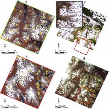
Fig. 2. Overview of the satellite scenes used in this study. (a) Northern and (b) southern ASTER scene, with overlapping parts indicated by a dashed line and used GCPs (circles) at sea level (blue) and above sea level (yellow). (c) TM scene of the study site using bands 3, 2 and 1 as RGB. The southern ASTER scene (d ctangle) is only partly coved. The close-up shows a gion with problematic seasonal snow in the TM scene. (d) The MSS scene with bands 3, 2 and 1 as RGB covers both ASTER scenes.
Table 1. Characteristics of the satellites and sensor used (NIR: near infrared; SWIR: shortwave infrared; TIR: thermal infrared; VNIR: visible and near infrared). Values in pantheses (5) indicate the number of summarized bands
ASTER has no blue band, and the spatial solution of the shortwave infrared (SWIR) bands (30 m) is diffent from the 15 m of the visible and near-infrared (VNIR) bands. In this study, the 30 m SWIR band AST4 was sampled to 15 m and smoothed with a Gaussian filter in order to duce its blocky appearance. The major advantage of the ASTER sensor with its along-track steo bands is the possibility of generating a DEM by steo corlation of the nadir- and back-looking infrared (IR) band (e.g. Reference ThompsonToutin, 2008). Only the TM sensor has a blue band for true-color image composites. The MSS sensor has neither a blue nor a SWIR band and a much coarser spatial solution (80 m). MSS is mainly used to determine glacier terminus positions but also for mapping glacier outlines when they a larger than about 0.5 km2. Additionally, digitized maps from the Glacier Atlas of Canada (scale 1 : 500 000) a fely available from Natural Resources Canada (http://www.atlas.nrcan.gc.ca). They we used to identify potential glaciers and to allocate the former ID codes to the glaciers under consideration.
Methodology
In general, the generation of glacier outlines can be divided into the steps: p-, main and post-processing. The pprocessing step includes data acquisition (download and file import), DEM generation/orthoctification (for ASTER) and the cation of various RGB (d, gen, blue) images (for quality control, manual corctions and LIA digitizing). The second step is the glacier mapping itself (band ratio and thshold selection, noise filter application and glacier map export). The final step is the cation of glacier outlines (raster–vector conversion) and application of corctions (e.g. for water, debris, clouds and shadow) as well as glacier basin digitization (hydrologic divides) and DEM fusion (for calculation of topographic inventory parameters). While the first step depends on the data source (e.g. steo capability of the sensor) and the softwa used, the main processing varies with the sensor (e.g. spectral and spatial solution) and the gion (e.g. cloud and snow conditions), and the post-processing depends on the intended application (e.g. cation of a first or updated inventory, analysis of changes, hydrologic calculations, natural hazards). General commendations for data processing and challenges lated to some of the points listed above a also discussed by Reference Paul, Kääb, Rott, Shepherd, Strozzi and VoldenRacoviteanu and others (2009). In the following, we thus focus on the issues lated to the processing in our study gion.
DEM generation
For each ASTER scene, a DEM was obtained from the 3N (nadir) and 3B (back-looking) bands at 30m cell size (DEM30). In both scenes, 32 ground control points (GCPs) we used. Additionally, 21 and 20 tie points we used for the northern and southern scene, spectively. DEM generation was done with the Orthoengine module of the PCI Geomatica 9.1 softwa. The height information was taken from four Canadian topographic maps at scale 1 : 250 000 (16D/E, 16K/L, 26I, 26H) and four maps at 1 : 50 000 (16E15, 16L02, 16L08, 16L15). The accuracy of the 1 : 250 000 and 1 : 50 000 maps is given horizontally as 125 and 25 m and vertically as 100 and 20 m, spectively. We used mountain peaks and points along the coast or at lakes as GCPs. While the GCPs in the northern scene a well distributed over the enti elevation range and scene (Fig. 2a), the GCPs in the southern scene a mo concentrated to the eastern sho (Fig. 2b). The overall horizontal root-mean-squa error (RMS x ,y ) was 1.87 pixels (northern scene) and 1.18 pixels (southern scene) and the sco of the pixel matching for the generated DEM was around 95%. The vertical error (RMS z ) at the collected GCPs was 90 m for the northern and 50m for the southern scene.
Major problems in the image matching, and thus in DEM generation, a (Fig. 3a and b): (1) atmospheric distortions (clouds, haze); (2) spectral featus (low contrast over water, detector saturation over clean snow/ice); (3) illumination (gions in shadow cast by the terrain or clouds); and (4) visibility (on steep north-facing slopes, invisible gions occur for the back-looking telescope). All four points together generate mismatched gions (i.e. data voids) and ‘artificial’ lief during the corlation process and automatic parallax-matching method (Reference Jacobs, Simms and SimmsKääb, 2002; Reference Suzuki, Fujita and AgetaToutin and Cheng, 2002). A strong corlation between elevation accuracy and slope has been found by Reference ToutinToutin (2002) which can be summarized as: the steeper the slope, the worse is the elevation accuracy. While low gain settings for the ASTER VNIR bands a a clear advantage for DEM cation over bright surfaces such as glaciers and snow, mo data voids have to be expected in gions of shadow due to missing contrast (Toutin, 2008). Moover, automated glacier mapping in shadow gions with low VNIR gain settings could be error-prone and might even pvent manual corction.
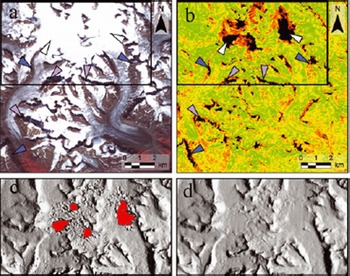
Fig. 3. (a) False-color composite of a subset of the southern ASTER scene and (b) sco channel ranging from high (gen) over low (d) to no (black) corlation in the pixel-matching process for the same gion as shown in (a). Problematic featus a indicated by arrows: shadow (violet), steep slopes (blue) and snow (white). (c, d) Hillshade psentation of (c) uncorcted (gaps a in d) and (d) corcted DEM.
Mismatched gions and artifacts we manually deleted and interpolated with the spatial interpolation tool provided by the softwa. Larger artifacts we common whe pixel matching was disturbed by steep terrain gradients, low contrast, and oversaturation (Fig. 3). Some pixels at the border of the DEM (around 10 pixels) and around voids in the DEM (<5 pixels) we deleted manually because of unalistic high-elevation values. For the latter, new heights we assigned using the spatial interpolation tool. Small artifacts and noise we duced with 3 by 3 (kernel size) Gaussian filters (a median filter led to similar sults).
As a further height verification, an additionally cated DEM with 60m cell size (DEM60) was extracted from the ASTER steo pairs, smoothed with a Gaussian filter, and sampled to 30 m cell size for better comparability with the DEM30. Indeed, the DEM60 has fewer data voids and artifacts, especially in gions of complex topography (ridges, peaks, steep slopes) and spectrally challenging terrain, such as low-contrast gions (snow and shadow), even though the is less detail. The two DEMs we compad and all cells which diffed vertically by >50m we deleted. These cells we assumed to be artifacts. New values we derived for these data voids using the spatial interpolation tools mentioned above. Other studies (e.g. Reference KääbKääb and others, 2003) used values from the DEM60 as a placement, but showed that only a weighted DEM fusion sults in a smooth transition between both DEMs. This approach was not applied he, as it is a challenging procedu. Orthoctification of the ASTER images was performed with the corcted ASTER DEMs using PCI Geomatica and the collected GCPs. The MSS and TM scenes we alady orthoctified by the Global Land Cover Facility (GLCF) from a diffent set of GCPs and DEM source. This sulted in a slightly diffent geolocation than achieved with the ASTER scenes and was manually adjusted in the Geographic Information System with ten additional tie points.
Glacier mapping with ASTER and MSS
The ideal satellite scene for glacier mapping: (1) is acquid at the end of the ablation period with as little seasonal snow as possible, (2) has a high solar position to avoid deep shadows, (3) includes a SWIR band for automated glacier mapping, and (4) is fe of clouds. An adequate spatial solution in spect to the size of the investigated glaciers (e.g. 10–30m pixels) is an additional advantage for a high classification accuracy (Paul and Kääb, 2005; Paul, 2007; Raup and others, 2007). Both investigated ASTER scenes a close to such optimal conditions, as only in the southern scene was seasonal snow psent, partly hiding the glaciers. The TM scene was partly foggy and the was too much seasonal snow at higher elevations to use it for aa change assessment (see close-up in Fig. 2c). At lower elevations, however, snow conditions we acceptable and clearly vealed the glacier terminus. Thus, this scene was used to assess length changes for a subsample of glaciers. Apart from the fact that MSS has no SWIR band and the spatial solution is much coarser than for TM or ASTER, the snow and atmospheric conditions for glacier detection we adequate (some fog in the eastern part was unproblematic). The MSS scene was thus used for both aa- and length-change assessment at a decadal scale.
Glacier mapping with ASTER and TM was done using thsholded band ratios (d/SWIR or NIR/SWIR) from the raw digital numbers, which has proved successful in other gions (e.g. Reference OmmanneyPaul and others, 2002; Paul and Kääb, 2005; Raup and others, 2007; Racoviteanu and others, 2008). An additional thshold in the gen or blue band was used to distinguish snow/ice in shadow from rock in shadow.
The pronounced spectral diffences of ice and snow in the SWIR band (very low flectance) compad to other surfaces form the base for automated glacier mapping (e.g. Reference Paul and SvobodaPaul, 2002; Reference BishopBishop and others 2004; Paul and Kääb, 2005). The ratios d/SWIR and NIR/SWIR with an appropriate thshold perform equally well, with slight diffences in the shadow (Reference Andassen, Paul, Kääb and HausbergAndassen and others, 2008). In shadow, the latter could misclassify vegetation and vealed problems at low solar elevations. For this ason, the new European Space Agency (ESA) project GlobGlacier (Paul and others, 2009) uses the d/SWIR ratio with an additional thshold in the gen (ASTER) or blue (TM/ETM+) band.
Since the is not much vegetation in the gion investigated he, no significant diffence between the band ratios is found. The thshold value for the ratio is very robust and is in most scenes investigated so far around 2.0 (±0.5). In this study, an ASTER scene with low gain settings in the VNIR bands is used, yielding a thshold value of 1.6. Mapping of glaciers in gions of shadow is mo sensitive to noise and depends on atmospheric conditions, solar elevation, diffuse flection from snow cover on adjacent slopes, etc. In this study, the AST1 thshold was set to 47 (AST1 > 47) to exclude rocks in shadow from the glacier classification. The sulting raster glacier map was converted to individual glacier polygons with the attributes ‘glacier’ or ‘no glacier’ using the methods described by Paul and others (2002).
For the MSS sensor (see Table 1 for spectral ranges), a decision-te classifier that utilizes multiple thsholds (Table 2) was used because MSS has no SWIR band (Fig. 4). Instead of a SWIR band, a NIR band was used for the band ratio (MSS3/MSS4). This method proved useful in mapping clean to slightly dirty ba ice and performed well in shadow gions (Fig. 4a). To move wrongly classified rocks in shadow, an additional thshold in the first NIR band (MSS3) was applied (Fig. 4b). Finally, the first the bands (MSS1–3) we used to map illuminated snow and clean ice (Fig. 4c). The sults we satisfying, except in some gions with cast shadow and debris on glaciers (Fig. 4d). He, the manual corction was mo difficult due to the duced spatial solution of MSS.
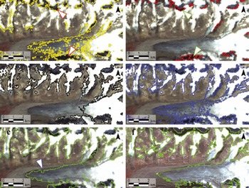
Fig. 4. Illustration of the glacier mapping with the MSS sensor: (a) MSS3/MSS4≥2 (d arrows denote misclassified rocks in shadow); (b) MSS3 < 20 (gen arrow points to rocks in shadow); (c) MSS 1–3 > 95; (d) unfilted glacier map; (e) median filted glacier map with uncorcted debris cover (blue arrow); and (f) for comparison, the median filted glacier outlines derived from the ASTER scene.
Table 2. Thresholds used for glacier mapping for all investigated sensors
A median filter (5 by 5 kernel size) was applied to the corcted glacier map for further noise duction (Fig. 4e) The filter duces misclassification due to noise in shadow, moves isolated pixels (snowfields), closes isolated gaps (rock outcrops or small debris/medial moraines), and very small glaciers (<0.1 km2) a decased in size (Fig. 5; Paul, 2007). Depending on the extent of medial moraines or abundant small snowfields, the kernel size can be varied. In this study, a kernel size of 5 by 5 was chosen, instead of the normally applied 3 by 3 kernel in other studies (e.g. Paul, 2002; Paul and others, 2002). All glacier maps (1975, 1990, 2000) we converted from raster grids into vector polygons for mo efficient data handling during post-processing.
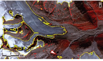
Fig. 5. Influence of the 5x5 median filter (d: moved, gen: added) on the classified glacier outline derived from ASTER (yellow). The d arrow points to a wrongly classified lake.
The major problems a encounted in glacier mapping which can be largely solved and a discussed in the following: (1) debris cover, (2) snowfields and (3) water bodies. Ice and snow in cast shadow is mapped accurately when an appropriate additional thshold in the gen or blue band is selected (Paul and Kääb, 2005). In order to illustrate the applied corctions, Figure 6a and b show an example of manually corcted debris cover for the ASTER and MSS sensor, spectively.
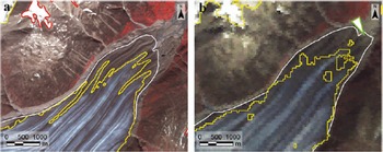
Fig. 6. Comparison of raw glacier outlines (yellow) with debris-cover corcted outlines (white) for (a) the ASTER scene and (b) the MSS scene. The d line in (a) marks a glacier that has been excluded; the gen arrow in (b) points to a gion whe the outline is highly uncertain.
1. Thick debris cover on glaciers has the same spectral properties as the debris or the rock walls surrounding the glacier and is thus classified as ‘non-glacier’. This is a general problem in automated glacier classification (e.g. Racoviteanu and others, 2009), and semi-automated methods for mapping debris-coved glacier parts have been proposed in several studies (e.g. Reference Bishop, Bonk, Kamp and ShroderBishop and others, 2001; Reference Paul, Kääb, Maisch, Kellenberger and HaeberliPaul and others, 2004; Reference BishopBolch and Kamp, 2006; Reference SolomonSuzuki and others, 2007). While these methods show promise, a high-quality DEM is needed and visual control and corction of the sults is quid nevertheless. For this ason, debris-coved parts we delineated manually in this study. This was straightforward with the comparatively high solution of the ASTER imagery (15 m), but much mo difficult with the coarser MSS solution (80 m) as indicated in Figure 6a and b. In total, corctions for debris cover have been applied to 167 glaciers. They we saved in a separate polygon layer and joined with the raw glacier map. The advantage of the separate debris layer is the possibility for later finements by subsequent analysis, a separate use for various modeling purposes (e.g. Reference RaupStokes and others, 2007) and better visualization of the applied corctions.
2. Snowfields a usually ‘misclassified’ as glaciers because they have the same spectral characteristics as the snow on the glaciers. In this study, glaciers we distinguished from snowfields by the psence of ba ice or based on morphological considerations. Small snowpatches (<0.02km2) we excluded by applying a size thshold. The method for moving larger snowpatches or those connected to glaciers is discussed below.
3. Most (turbid) water bodies (e.g. ocean, lakes, rivers) a misclassified as glaciers. This is easily corcted, as they a clearly visible in the RGB images cated during pprocessing, even if their surface is frozen. The water bodies we dictly edited in the vector glacier layer using a false-color composite with the VNIR bands AST 3, 2 and 1 (as RGB) in the background.
All clearly visible and identifiable LIA moraines and trimlines we manually delineated for a total of 264 glaciers to derive changes in length and aa since the LIA. These we stod as separate polygons, and appended to the year 2000 glacier extent mapped from ASTER scenes. For most glaciers and some ice caps, the delineation is straightforward (Reference ToutinWolken, 2006), but lichen-fe zones might also sult from persistent snowfields (Reference Kaser, Cogley, Dyurgerov, Meier and OhmuraKoerner, 1980). We tried to exclude such doubtful fofields in this assessment. Further details of the LIA-extent mapping a given by Paul and Kääb (2005).
Glacier basin delineation
The definition of glacier entities is crucial for the location of drainage divides, calculation of topographic glacier parameters and for change assessment (e.g. Reference Bolch and KampDowdeswell and others, 1995). This definition is especially challenging for complex glacier systems (e.g. compound glaciers, coalescing glaciers, or ice caps with complex topologies) which a often found in the study gion. From a glaciological point of view, it has to be consided that the (hydrologic) division of an ice cap into separate units could be questionable. As this strongly depends on the topology or shape of the ice cap, this has to be decided on a case-by-case basis. In this study, glaciers we separated according to their drainage systems as proposed by the UNESCO guidelines (Müller and others, 1977) and the GLIMS data analysis tutorial (B. Raup and S.J. Singh Khalsa, http://www.glims.org/MapsAndDocs/assets/GLIMS_Analysis_Tutorial_a4.pdf). Contiguous ice masses we split along the topographic divides if flow between the individual parts could be neglected. The DEMs and the aspect grids helped to determine the location of ice divides, but failed in flat parts of joint accumulation aas of compound glaciers (Fig. 7a and b). In that case, the location of the divides was estimated based on illumination diffences and glaciological interptation (Racoviteanu and others, 2009). Uncertainty in the location of the divides is indicated by digitizing straight lines as suggested by Paul and Kääb (2005). In cases whe small glacier parts we flowing into other drainage systems than the main glacier, they we counted as parts of the larger glacier (Fig. 7a). Glacier basins include all glacier parts that a counted as one entity (year 2000 extent) in the glacier inventory.
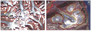
Fig. 7. Glacier basins (d lines) and flow dictions (black arrows) for two critical gions. (a) A system of valley glaciers with adjacent accumulation aas. Uncertain divisions a indicated by straight lines (blue arrows); a glacier that contributes mass by ice avalanches (gen arrow), and a formerly connected tributary glacier (orange arrow) a also marked. (b) Glacier divides on a mixed ice-cap/valley-glacier system with flow dictions into diffent drainage basins. The critical division along the topographic divide is marked with a blue arrow; glacier outlines a in yellow and 100m contour intervals a in gen.
In many cases, (seasonal) snowfields or avalanche deposits a found that cross the LIA lateral moraines (in the ablation aa) or hide the perimeter of the accumulation aa. The glacier basins a also used to separate these snowfields from the main glacier. Due to the overlap, the delineation could be challenging (the basins should be outside the LIA moraines) and introduces some uncertainty in the accumulation aa in absolute terms. However, this positional inaccuracy does not influence the aa changes calculated he, because all glacier extents (LIA, 1975, 1990, 2000) fer to the same divides. Pennial snowfields and possible glaciers that a nearly completely snow-coved in the ASTER scene a excluded from the analysis due to the high uncertainties of their true extent (Fig. 6a). However, for submission to the GLIMS glacier database we intend to include them again in a clearly marked form.
All basins we delineated as polygons and identified by glacier IDs which we digitized manually from the maps of the Glacier Atlas of Canada (http://atlas.gc.ca/). Since those glacier IDs we not compliant with the World Glacier Monitoring Service IDs, both IDs we assigned to the spective basins. Because the Glacier Atlas of Canada also contained pennial snowfields, the number of entities in the atlas far exceeds the number of glaciers mapped in this study. Hence, only the IDs from the Glacier Atlas of Canada we taken into account and finally joined with the glacier basins that corspond most closely with the glacier outlines. All glaciers we numbed sequentially according to the World Glacier Inventory numbering system (e.g. Reference Hall, Bayr, Schöner, Bindschadler and ChienHoelzle and Trindler, 1998). In a final step, the corcted glacier map was intersected by the glacier basins to obtain individual glacier entities (total 662 glaciers) with corsponding glacier IDs.
Flowlines
The roughness of the DEM and curvatu changes down-glacier did not allow the automated extraction of flowlines. Thus, hypothetical flowlines we digitized manually to determine total glacier length and length changes. Digitization starts at the lowest point of a glacier and follows a central flowline until the highest point is ached. Ideally, the line crosses the contour lines perpendicularly, and crosses the tongues of all available glacier extents at their furthermost end. The major challenge was thus to identify one central flowline for each glacier and all its tributaries. Although contour lines we used as a visual support, it was not possible to delineate flowlines for all glaciers and ice caps. Finally, the flowlines we intersected with all glacier extents, sulting in the following number of flowline segments: length of the year 2000 (254 lines), length change 1990–2000 (139 lines), length change 1975–2000 (168 lines) and length change LIA–2000 (208 lines).
Results and Discussion
After all, two DEMs we extracted from the ASTER scenes, and for each point in time (LIA, 1975, 1990, 2000) one corcted glacier map was derived. The year 1990 glacier map was only used to extract length changes. The digitized LIA extents we appended to the year 2000 extents, so the diffences between the two extents a clearly visible (Fig. 8). The further DEM-derived raster grids (aspect, slope, hypsography), the statistical analysis of the derived glacier inventory, and further derived parameters a psented in part II of this study (Reference MethodsPaul and Svoboda, 2009).
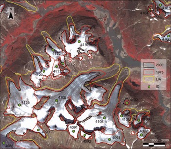
Fig. 8. Example of glacier-mapping sults showing the LIA, MSS and ASTER extents (see legend for colors). The ID numbers fer to the Canadian glacier inventory (http://atlas.gc.ca/).
After the corctions mentioned above have been applied to the ASTER DEM, its quality is sufficient for the purpose of orthoctifying the scenes and deriving glacier parameters. Even though the a many sources of error in the DEM extraction, they do not interfe too much with the sults for the topographic glacier parameters. Most of the errors concern: (1) flat parts of glaciers in the snow-coved accumulation aa, (2) steep slopes whe glaciers a seldom found or (3) sharp ridges/csts. However, the quality of the DEMs was too poor to use them for automated debris-cover mapping according to the methods proposed in the studies mentioned above. The automated cognition of basin divides (watershed analysis) performed poorly as well, but cently developed methods for automated glacier basin delineation (Reference KoernerManley, 2008) have not been tested yet. In the futu, high-solution radar or laser DEMs might help to improve the situation (IGOS, 2007).
The main aim of this study was to cate a new glacier inventory for part of Cumberland Peninsula, including mapping of LIA extents and the lated assessment of changes in length and aa. As the TM scene had too much seasonal snow and only coved two-thirds of the gion, it was only used as an additional point in time for length-change assessment. Unfortunately, we did not find a better scene in the archives for this gion and that period (1990s). Glacier mapping and length-change assessment with MSS is less accurate due to the lack of a SWIR band and the duced spatial solution (80 m). The comparatively low solution of the MSS sensor made it difficult to identify the glacier terminus and thus to map the debris-coved glacier parts. Similar problems we ported by Reference HaeberliHall and others (2003) for a larger debris-coved glacier in Austria (Pasterzenkees). The problem of glacier mapping in shadow gions could be solved by combining the glacier map from MSS with that from ASTER. It is thus assumed that no change has taken place in the upper (shadowed) parts of the accumulation aa for those glaciers. To pserve the accuracy of the ASTER-derived glacier map, the LIA extent was appended to the year 2000 extent, instead of the MSS-derived 1975 extent.
Due to the missing SWIR channel of MSS, we developed a mapping algorithm that classifies glaciers with multiple thsholds. The mapping was successful except for strongly (i.e. optically thick) debris-coved ice and slightly debris-coved ice in shadow. The manual editing is hamped by the spatial solution of the sensor (80 m). However, the semi-automated technique provides glacier outlines for clean ice much faster and mo consistently than digitizing by hand. MSS scenes a available for most parts of the world with an archive going back to 1972. They will be especially intesting for assessment of length and aa changes in mote gions with larger glaciers.
Mapping of debris-coved gions is subject to large errors because even in the field it is sometimes difficult to determine whether or not ice exists under the debris. This is particularly the case in gions of shadow and near the terminus when the tongue is flat or collapsing and not well structud (cf. Paul and Kääb, 2005). The accuracy of the delineation also depends on the solution of the images and the morphology of the glacier (Fig. 6). Thefo, debris cover was delineated in this study by individual polygons befo a union with the automatically classified glacier outlines was applied. This also allows automated assignment of diffent accuracy levels to debris-coved and clean ice.
Even mo delicate and complex than debris-cover delineation is the delineation of ice divides in the accumulation gion whe the quality of the DEM from optical sensors is poor (Fig. 3). In a study on ice caps in the Russian Arctic, Reference Dowdeswell and GlazovskyDowdeswell and others (1995) used illumination diffences on satellite images with low solar elevations to define principal drainage divides of ice caps. While this method might also work well for the ice caps in the gion studied he, the elevation diffences in the accumulation gions of connected valley glaciers a likely too small. It is expected that a DEM from radar or laser sensors would help to determine local culminations and flow dictions in this gion. Such DEMs, which a curntly not available for the study site, would also improve the digitizing of flowlines and the quality of extracted glacier parameters, at least when they have been acquid in the same year as the satellite scene. The a some advantages in storing glacier basins as separate polygon datasets: (1) The basins can be constructed and edited later, (2) the same basin layer can be applied to diffent (orthoctified) datasets, (3) they allow selection of specific samples of glaciers, and (4) a common ID can be applied to glacier groups (e.g. including all entities belonging to a former LIA glacier).
The most accurate estimation of glacier tat is clearly from the mapped LIA position to the year 2000. First, the distances a long, and second the delineation of both extents was based on the high-solution ASTER image. The terminus positions from 1990 a also pcise (±1 pixel), even though the length changes to 2000 a mostly small. The error of the 1975–2000 length change is, because of the coarser MSS sensor solution, about two to the times larger (±3 pixels) than for the other two sensors (Reference HaeberliHall and others, 2003). Also he the glaciological interptation could introduce much higher errors than lated to the technical questions discussed above. This particularly applies to the length change since the LIA, as the location of the split from the tributaries could be inaccurate by several hundd meters. Of course, for this study we selected only those glaciers whe the situation is clear, but this might be an important point to consider in futu studies.
A statistically sound estimate of the mapping accuracy is difficult to calculate for several asons:
All outlines we alady compad and corcted against a ground truth (the used satellite scene). Thus, an independent ground control for error calculation is not available.
Higher-solution datasets (e.g. aerial photography, IKONOS or QuickBird satellite data) can only be used for comparison when the images have been acquid at the same date (week), which is seldom the case. Moover, due to the missing SWIR band the delineation is mo challenging and details a interpted diffently. Thus, statistical rigor is missing in such comparisons.
On any given image and for clean glaciers, the automatically derived outlines a superior to manually digitized outlines for at least two asons: the method is consistent with spect to the spectral properties (the same ratio thshold applies to all pixels) and the shape of the outline is not generalized. Both points a important to guarantee producible sults.
Another levant issue to consider is that the glaciological uncertainty (e.g. lated to the corct position of basin divides, separation from seasonal snowfields, or delineation of debris cover) is much higher than the technical accuracy of the applied glacier-mapping method. As pvious comparisons of diffent methods have shown (e.g. Paul and Kääb, 2005), they could be distinguished only at the level of individual pixels or the workload quid for p- and post-processing (e.g. manual corctions). The ‘error’ of the mapping method thus has little influence on the accuracy of the final glacier outline.
The estimation of the end of the LIA on Cumberland Peninsula is uncertain. Reference Stokes, Popovnin, Aleynikov, Gurney and ShahgedanovaThompson (1954) showed with lichen analysis that the glaciers we still advancing around 1880 near the study site. Furthermo, several studies estimated that a mo pronounced glacier tat started no earlier than 1920, as a rapid warming was observed after that time (Bird, 1967; Reference Andws and BarryAndws and Barry, 1972; Andws, 2002). This uncertainty is discussed in mo detail in part II of this study (Paul and Svoboda, 2009), whe we calculate mean annual mass changes.
Conclusions
In this part of the study, we have psented the methods and challenges for mapping glaciers from the optical sensors (ASTER, TM, MSS) in a mote gion in the Canadian Arctic (Cumberland Peninsula, Baffin Island). For all sensors, semi-automated mapping methods have been applied, and the datasets quid to cate a detailed glacier inventory and calculate changes in length and aa have been psented. Regarding the now fe availability of the enti Landsat archive (US Geological Survey, http://pubs.usgs.gov/fs/2008/3091/pdf/fs2008-3091.pdf) we look forward to the application of the methods psented he in diffent parts of the world. Mo specifically, the following conclusions a drawn:
The selection of suitable images from any of the sensors investigated he is challenging in this Arctic gion due to adverse weather conditions (fquent clouds, early snow) near the end of the ablation period and the narrow time window with optimal conditions.
ASTER is a very suitable sensor to map even small glaciers at the basin scale. Combined with the possibility to cate a DEM from its along-track steo band, ASTER allows the compilation of data for a detailed glacier inventory (including topographic parameters) in mote gions.
The quality of the DEM is duced in gions with low contrast (snow, shadow) whe data voids occur. These gions can be improved by internal measus (e.g. a 60m DEM, interpolation tools).
The Landsat TM (or ETM+) sensor has the advantages over ASTER of covering a gion that is nine times larger and having a band in the blue part of the spectrum which facilitates glacier mapping in shadow gions.
Automated glacier mapping with band ratios is a fast, robust, accurate and straightforward method that can be highly commended for (global) application. It might even be pferable over manual digitization (for debris-fe ice), as it is producible, consistent and without generalization.
A semi-automated glacier-mapping method (decision-te classifier), developed for the MSS sensor, performed well even though the SWIR band is missing. Due to the coarser spatial solution (80 m), mo intense manual corctions have to be carried out (debris cover, snowfields) and the accuracy of the total aa and the derived length changes is duced. A minimum glacier size of about 0.1 km2 can be mapped.
Of particular intest for change assessment with MSS is its long historic archive dating back to 1972.
Major challenges to achieve accurate sults a lated to issues of glaciological interptation (e.g. location of ice divides, interptation of debris cover, attached seasonal snow, deep shadows), rather than the technical accuracy of the method used for glacier classification.
Keeping the raw and corcted glacier outlines as well as the basins in separate vector layers allows very efficient and consistent data handling (e.g. garding later corctions, exclusion of attached snowfields, consideration of former extents, and further applications). Moover, the separate basin layer could be applied to further (orthoctified) datasets and used to apply joint codes.
The average time quid for corcting and pparing one glacier (terminus, debris, flowline, basins) is around 10 min. An additional 5 min per glacier has to be taken into account to delineate the LIA extents.
Acknowledgements
We thank A. Racoviteanu and an anonymous viewer for constructive comments, and the scientific editor G. Cogley for caful editing and suggestions. The study was funded by the ESA project GlobGlacier (21088/07/I-EC) and has been performed within the framework of the GLIMS initiative. GLIMS also provided the ASTER imagery used in this study. The TM and MSS scenes we obtained from the GLCF at the University of Maryland, USA.


