


Impact Statement
Uncertainty quantification via machine learning is a vibrant area of research, and many methods have been proposed. Here, we describe and demonstrate a simple method for adding uncertainty to most any neural network (a type of machine learning algorithm) regression task. We demonstrate the utility of this method by predicting tropical cyclone intensity forecast uncertainty. The method is intuitive and straightforward to implement with standard machine learning software. The authors believe it will become a powerful, go-to method moving forward.
1. Introduction
Uncertainty quantification via machine learning methods is a vibrant area of research (e.g., Sensoy et al., Reference Sensoy, Kaplan and Kandemir2018; Amini et al., Reference Amini, Schwarting, Soleimany and Rus2019), and many methods for uncertainty estimation via artificial neural networks have been proposed (e.g., Abdar et al., Reference Abdar, Pourpanah, Hussain, Rezazadegan, Liu, Ghavamzadeh, Fieguth, Cao, Khosravi, Acharya, Makarenkov and Nahavandi2021; Jospin et al., Reference Jospin, Laga, Boussaid, Buntine and Bennamoun2022). Many studies have focused on uncertainty quantification for classification; however, problems in the earth sciences are often framed in terms of regression tasks (i.e., estimating continuous values). For example, scientists might wish to estimate how much it will rain tomorrow, the peak discharge of a river next year, or the thickness of an aquifer at a set of locations. Estimates of the uncertainty associated with the predicted values are necessary to formulate policy, make decisions, and assess risk.
Here, we describe and demonstrate a simple method for adding uncertainty to most any neural network regression architecture. The method works by tasking the network to locally predict the parameters of a user-specified probability distribution, rather than just predict the value alone. Although the approach was introduced decades ago (Nix and Weigend, Reference Nix and Weigend1994, Reference Nix, Weigend, Tesauro, Touretzky and Leen1995) and is a standard in the computer science literature (e.g., Sountsov et al., Reference Sountsov, Suter, Burnim and Dillon2019; Duerr et al., Reference Duerr, Sick and Murina2020), it is much less known in the earth science community. A few applications of the method appear in the recent literature (e.g., Barnes and Barnes, Reference Barnes and Barnes2021; Foster et al., Reference Foster, Gagne and Whitt2021; Guillaumin and Zanna, Reference Guillaumin and Zanna2021; Gordon and Barnes, Reference Gordon and Barnes2022), but all of these focus strictly on the Gaussian distribution.
The Gaussian distribution has the benefits of familiarity and the comforts of common use. Nonetheless, the Gaussian distribution is sorely limiting due to its symmetry and fixed tailweight. In the earth sciences, uncertainty is often asymmetric. Consider the prediction of strictly positive quantities such as rain intensity, stream discharges, contaminant concentrations, and wind speeds. There is a chance that the true value is greater than twice the predicted value, but there is never any chance that the true value is less than zero.
Here, we formulate neural network regression with uncertainty quantification using the sinh-arcsinh-normal distribution (Jones and Pewsey, Reference Jones and Pewsey2009, Reference Jones and Pewsey2019). While two parameters define a Gaussian distribution (location and scale), the sinh-arcsinh-normal distribution is defined by four parameters (location, scale, skewness, and tailweight). This method for incorporating uncertainty with the sinh-arcsinh-normal distribution (which we call SHASH) is understandable, surprisingly general, and simple to implement with confidence. The sinh-arcsinh-normal distribution is certainly not the only choice of distribution for environmental problems, and in fact, there may be better-suited distributions depending on the specific application. Here, we merely wish to demonstrate the utility of the sinh-arcsinh-normal distribution for capturing asymmetric uncertainties in predicting hurricane intensity errors. Overall, we believe that this simple method for adding uncertainty using a user-defined distribution will become a powerful go-to approach moving forward.
2. Data
The data set for this study is based on how forecasters at the National Weather Service (NWS) National Hurricane Center (NHC) in Miami make their subjective forecasts of the tropical cyclone maximum sustained surface wind (intensity) out to 5 days. Several objective models provide intensity forecast guidance, and verification results show that the equally weighted consensus of the best-performing individual models is often the most accurate (Cangialosi, Reference Cangialosi2022). The consensus model (Consensus from here on out) provides a first-guess intensity; then forecasters will lean their forecast more toward individual models they feel best handle the tropical cyclone based on the current forecast situation.
For the 2021 Hurricane Season, NHC’s primary equally weighted intensity consensus model (IVCN) consisted of the following five forecast models: (1) The Decay-Statistical Hurricane Intensity Prediction Scheme (DSHP); (2) The Logistic Growth Equation Model (LGEM); (3) The Hurricane Weather Research and Forecast Model (HWRF); (4) The Hurricanes in a Multiscale Ocean-coupled Non-hydrostatic (HMON) Model; and (5) The U.S. Navy’s Coupled Ocean–Atmosphere Mesoscale Prediction System for tropical cyclones (CTCX). LGEM and D-SHIPS are statistical-dynamical models, while HWRF, HMON, and CTCX are regional dynamical models. Although not included in IVCN, intensity forecasts from several global models, such as the National Weather Service Global Forecasting System (GFS), are also used for the NHC official forecast. Cangialosi et al. (Reference Cangialosi, Blake, DeMaria, Penny, Latto, Rappaport and Tallapragada2020) provide more detailed descriptions of these intensity models and others used by NHC.
To mimic NHC’s subjective forecast, four intensity guidance models were chosen as input to the neural network. The models are usually updated every year, so the error characteristics are not stationary. Therefore, it is not possible to go back too far into the past for training samples. On the other hand, a reasonably large training sample is required, so the model input from at least a few years is needed. As a compromise between these two factors, the training data set includes the DSHP, LGEM, HWRF, and GFS intensity forecasts from 2013 to 2021. The CTCX and HMON models were not included, because those were not consistently available back to 2013.
To ensure time consistency across time zones, NWS data collection and forecasts are based on “synoptic” times, which are at 00, 06, 12, and 18 UTC. NHC forecasts are issued every 6 hr at 3 hr after synoptic times, so the guidance models are also run every 6 hr. However, the dynamical HWRF and GFS models are not available until after the NHC forecast is issued. To account for the delayed model guidance, the forecasts from the previous 6-hr cycle are interpolated to the current synoptic time. These are referred to as “interpolated” models and are designated as HWFI and GFSI for the HWRF and GFS, respectively. The network training includes only the interpolated models so that it is relevant to what forecasters would have available when they make their forecasts. The statistical D-SHIPS and LGEM models use input from previous forecast cycles and so are available when the forecasters are making their predictions. Although the NHC forecast is at 12-hr intervals out to 3 days and then every 24 hr thereafter, for simplicity, only the input at 24-hr intervals is considered in this study.
Again following the NHC forecast procedure, the input to the network is the deviation of each of the four input models (DSHP, LGEM, HWFI, GFSI) from the equally weighted average intensity (henceforth, termed Consensus) from these same four models. Sometimes the forecast from a particular model does not extend to 5 days. This can happen, for example, if the model forecast moves the storm over land or very cold water and the tropical cyclone dissipates. For a case to be included in the training sample at a given forecast period, at least two of the four input models must be available. The intensity forecast for the missing models is set to the average of the available models and the number of models available is provided as input to the network (NCI).
Several studies have shown that the performance of NHC’s intensity guidance models depends on the forecast situation (e.g., Bhatia and Nolan, Reference Bhatia and Nolan2015). To allow the network’s prediction of the intensity error distributions to account for this variability, several forecast-specific parameters are also included as input. These consist of the observed intensity at the start of the forecast (VMAX0), the magnitude of the storm environment 850 to 200 hPa wind shear vector (SHDC), the sea surface temperature at the tropical cyclone center (SSTN), the distance of the storm center from land (DTL), the storm latitude (SLAT), the intensity change in the 12 hr prior to the forecast initialization time (DV12), and the intensity of the Consensus (VMXC). The 12 hr prior intensity change is the same for all forecast times. All of the other parameters are averaged over the 24-hr period ending at the forecast time. All of the forecast additional parameters are obtained from the diagnostics calculated as part of the DSHP statistical-dynamical model.
NHC has forecast responsibility for all tropical cyclones in the North Atlantic (AL) and eastern North Pacific (EP) to 140 W. The NWS Central Pacific Hurricane Center (CPHC) in Honolulu has forecast responsibility for the central North Pacific (CP), which extends from 140 W to the dateline. Because the boundary between the EP and CP is not meteorologically significant, the EP and CP samples are combined. The Department of Defense Joint Typhoon Warning Center has the U.S. forecast responsibility for tropical cyclones over the rest of the globe. These tropical cyclones are not considered in this study.
The ground truth for verification of the NHC and CPHC intensity forecasts is from the “Best Track” data, which is a post-storm evaluation of all available information (Landsea and Franklin, Reference Landsea and Franklin2013). The Best Track includes the track, maximum wind, and several other tropical cyclone parameters every 6 hr. One of the other parameters is the storm type, which sometimes includes a portion of the life cycle when tropical cyclones become extratropical cyclones. We excluded the extratropical portion of the tropical cyclones in our data set. The tropical cyclone intensity in the Best Track is almost never lower than 20 knots, so this is a lower bound on the forecast.
We task a neural network to take in the 12, single-valued predictors (see Table 1) and predict the unweighted Consensus error of the tropical cyclone intensity forecast at lead times of 24, 48, 72, 96, and 120 hr. The network does not output a deterministic prediction of the error, but rather, the network is designed to output a conditional probability distribution that represents a probabilistic prediction of the Consensus error. We train separate networks for the Atlantic (AL) and the East/Central Pacific (EPCP) but at time present their results in the same figure. In Section 3, we will discuss the form of the probability distribution and how it is trained. In Section 5, we will present the results.
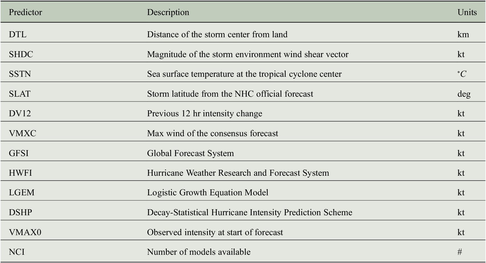
Table 1. Summary of the 12 predictors used in the model.
3. Sinh-arcsinh-normal distribution
Here, we demonstrate the use of the sinh-arcsinh-normal (SHASH) distribution (Jones and Pewsey, Reference Jones and Pewsey2009, Reference Jones and Pewsey2019) to add uncertainty to neural network regression tasks. The SHASH takes four parameters in TensorFlow 2.7.0 (Abadi et al., Reference Agarwal, Barham, Brevdo, Chen, Citro, Corrado, Davis, Dean, Devin, Ghemawat, Goodfellow, Harp, Irving, Isard, Jozefowicz, Jia, Kaiser, Kudlur, Levenberg, Mané, Schuster, Monga, Moore, Murray, Olah, Shlens, Steiner, Sutskever, Talwar, Tucker, Vanhoucke, Vasudevan, Viégas, Vinyals, Warden, Wattenberg, Wicke, Yu and Zheng2015): location ( $ \mu $
), scale (
$ \mu $
), scale ( $ \sigma $
), skewness
$ \sigma $
), skewness $ \left(\gamma \right) $
, and tailweight (
$ \left(\gamma \right) $
, and tailweight ( $ \tau $
) and provides a basis for representing state-dependent, heteroscedastic, and asymmetric uncertainties in an intuitive manner (Duerr et al., Reference Duerr, Sick and Murina2020). The SHASH may be symmetric, but it may be highly asymmetric with a weighted tail (unlike a normal distribution). The SHASH also allows for non-positive values (unlike a log-normal distribution). For our specific application, tropical cyclone intensity errors can be positive or negative, and can be skewed toward the positive tail under certain conditions. These state-dependent, heteroscedastic, and asymmetric uncertainties in the intensity error can thus be approximated as different SHASH distributions for every hurricane intensity forecast. Examples of the family of SHASH distributions are shown in Figure 1, of which the normal distribution is a special case (skewness
$ \tau $
) and provides a basis for representing state-dependent, heteroscedastic, and asymmetric uncertainties in an intuitive manner (Duerr et al., Reference Duerr, Sick and Murina2020). The SHASH may be symmetric, but it may be highly asymmetric with a weighted tail (unlike a normal distribution). The SHASH also allows for non-positive values (unlike a log-normal distribution). For our specific application, tropical cyclone intensity errors can be positive or negative, and can be skewed toward the positive tail under certain conditions. These state-dependent, heteroscedastic, and asymmetric uncertainties in the intensity error can thus be approximated as different SHASH distributions for every hurricane intensity forecast. Examples of the family of SHASH distributions are shown in Figure 1, of which the normal distribution is a special case (skewness $ \gamma =0 $
, tailweight
$ \gamma =0 $
, tailweight $ \tau =1 $
; orange curve in Figure 1b). A detailed description of the SHASH formulation and implementation is provided in Appendix B.
$ \tau =1 $
; orange curve in Figure 1b). A detailed description of the SHASH formulation and implementation is provided in Appendix B.
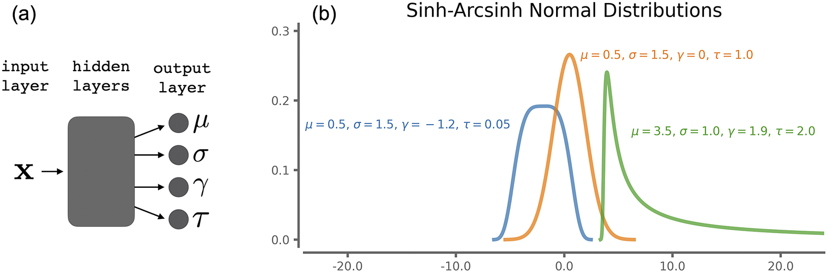
Figure 1. (a) Neural network architecture and (b) example sinh-arcsinh-normal (SHASH) distributions for combinations of parameters.
The neural network is tasked with predicting the four parameters of the SHASH distribution (Figure 1a). That is, the output of the network contains four units capturing $ \mu, \sigma $
,
$ \mu, \sigma $
, $ \gamma $
, and
$ \gamma $
, and $ \tau $
. The parameters
$ \tau $
. The parameters $ \sigma $
(scale) and
$ \sigma $
(scale) and $ \tau $
(tailweight) must be strictly positive. To accomplish this, we follow a common trick in computer science (Duerr et al., Reference Duerr, Sick and Murina2020) to ensure that
$ \tau $
(tailweight) must be strictly positive. To accomplish this, we follow a common trick in computer science (Duerr et al., Reference Duerr, Sick and Murina2020) to ensure that $ \sigma $
and
$ \sigma $
and $ \tau $
are always strictly positive by tasking the network to predict the
$ \tau $
are always strictly positive by tasking the network to predict the $ \log \left(\sigma \right) $
and the
$ \log \left(\sigma \right) $
and the $ \log \left(\tau \right) $
rather than
$ \log \left(\tau \right) $
rather than $ \sigma $
and
$ \sigma $
and $ \tau $
themselves. Here, we predict the four parameters of the SHASH distribution using fully connected neural networks. However, a benefit of this general approach for including uncertainty is that it can be easily applied to most any neural network architecture, as it only requires modification of the output layer and the loss function (see Section 3.1).
$ \tau $
themselves. Here, we predict the four parameters of the SHASH distribution using fully connected neural networks. However, a benefit of this general approach for including uncertainty is that it can be easily applied to most any neural network architecture, as it only requires modification of the output layer and the loss function (see Section 3.1).
3.1. The loss function
The neural network architecture shown in Figure 1a trains using the negative log-likelihood loss defined for the ith input sample, $ {x}_i $
, as
$ {x}_i $
, as
 $$ \mathrm{\mathcal{L}}\left({x}_i\right)=-\log {p}_i. $$
where $ {p}_i $
is the value of the SHASH probability density function,
$ {p}_i $
is the value of the SHASH probability density function, $ \mathcal{P} $
, with predicted parameters
$ \mathcal{P} $
, with predicted parameters $ \left(\mu, \sigma, \gamma, \tau \right) $
evaluated at the true label
$ \left(\mu, \sigma, \gamma, \tau \right) $
evaluated at the true label $ {y}_i $
. That is,
$ {y}_i $
. That is,
 $$ {p}_i=\mathcal{P}\left({y}_i|\hskip0.3em ,\mu, \sigma, \gamma, \tau \right). $$
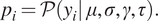
Figure 2 shows schematically how the probability $ {p}_i $
depends on the specific parameters of the distribution predicted by the network. For example, if the predicted distribution is overconfident (the distribution’s width is too small),
$ {p}_i $
depends on the specific parameters of the distribution predicted by the network. For example, if the predicted distribution is overconfident (the distribution’s width is too small), $ {p}_i $
will be small and the loss
$ {p}_i $
will be small and the loss $ \mathrm{\mathcal{L}} $
will be large (Figure 2a). If the network is underconfident (the distribution’s width is too large),
$ \mathrm{\mathcal{L}} $
will be large (Figure 2a). If the network is underconfident (the distribution’s width is too large), $ {p}_i $
will also be small and the loss
$ {p}_i $
will also be small and the loss $ \mathrm{\mathcal{L}} $
will once again be large (Figure 2b). Like Goldilocks, the network needs to get things “just right,” by properly estimating its uncertainty to obtain its best guess. Better predictions are associated with larger
$ \mathrm{\mathcal{L}} $
will once again be large (Figure 2b). Like Goldilocks, the network needs to get things “just right,” by properly estimating its uncertainty to obtain its best guess. Better predictions are associated with larger $ {p}_i $
, and thus smaller loss
$ {p}_i $
, and thus smaller loss $ \mathrm{\mathcal{L}} $
(Figure 2c). Note that this approach is directly tied to the standard method of parameter estimation in statistics known as maximum likelihood estimation (Duerr et al., Reference Duerr, Sick and Murina2020).
$ \mathrm{\mathcal{L}} $
(Figure 2c). Note that this approach is directly tied to the standard method of parameter estimation in statistics known as maximum likelihood estimation (Duerr et al., Reference Duerr, Sick and Murina2020).
Figure 2. Schematic showing how the loss function probability $ {p}_i $
is dependent on the predicted probability distribution.
$ {p}_i $
is dependent on the predicted probability distribution.
While this work highlights the sinh-arcsinh-normal probability density function, the loss function in Eq. (1) can be used for any well-behaved probability distribution. The trick to training the neural network is that the loss for observation $ i $
is the predicted probability density function evaluated at the observed
$ i $
is the predicted probability density function evaluated at the observed $ {y}_i $
. For example, if the
$ {y}_i $
. For example, if the $ y $
variable denotes a percentage or proportion, then a distribution with finite support from
$ y $
variable denotes a percentage or proportion, then a distribution with finite support from $ 0 $
to
$ 0 $
to $ 1 $
may be more appropriate. The beta and Kumaraswamy are two such distributions that have been used to model hydrological variables such as daily rainfall (e.g., Mielke, Reference Mielke1975; Kumaraswamy, Reference Kumaraswamy1980). Even so, we believe that the SHASH offers a versatile, intuitive family of distributions that will likely be applicable to a wide range of earth science applications.
$ 1 $
may be more appropriate. The beta and Kumaraswamy are two such distributions that have been used to model hydrological variables such as daily rainfall (e.g., Mielke, Reference Mielke1975; Kumaraswamy, Reference Kumaraswamy1980). Even so, we believe that the SHASH offers a versatile, intuitive family of distributions that will likely be applicable to a wide range of earth science applications.
3.2. Network architecture and training specifics
For all SHASH prediction tasks, we train a fully connected neural network (abbreviated throughout as NN) with two hidden layers of 15 and 10 units, respectively, to predict the first three parameters of the SHASH distribution (i.e., $ \mu, \sigma, \gamma $
). We found that including the tailweight
$ \mu, \sigma, \gamma $
). We found that including the tailweight $ \tau $
did not improve the network performance, and so we set
$ \tau $
did not improve the network performance, and so we set $ \tau =1.0 $
throughout. The rectified linear activation function (ReLu) is used in all hidden layers. We train the network with the negative log-likelihood loss given in Eq. (1) using the Adam optimizer in TensorFlow with a learning rate of
$ \tau =1.0 $
throughout. The rectified linear activation function (ReLu) is used in all hidden layers. We train the network with the negative log-likelihood loss given in Eq. (1) using the Adam optimizer in TensorFlow with a learning rate of $ 0.0001 $
and batch size of 64. The network is trained to minimize the loss on the training data, and training is halted using early stopping when the validation loss has not decreased for 250 epochs. When this occurs, the network returns the network weights associated with the best validation loss.
$ 0.0001 $
and batch size of 64. The network is trained to minimize the loss on the training data, and training is halted using early stopping when the validation loss has not decreased for 250 epochs. When this occurs, the network returns the network weights associated with the best validation loss.
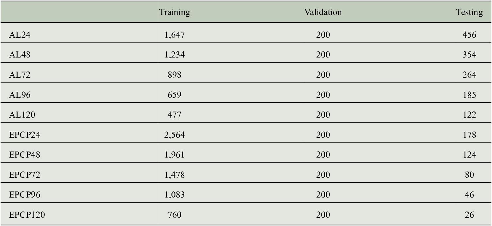
The data is split into training, validation, and testing sets. To explore the sensitivity of the results to the random training/validation split as well as the randomly initialized weights, each network setup is trained five different times using five different random seeds. Testing results are then shown for the network with the lowest validation error of the five. In addition, we train five different networks for each possible nine testing years (from 2013 to 2021). Figures 3–5 show case studies and results for one specific network using a random seed of 739 for testing year 2020 to provide readers with specific examples. In this case, the testing set is composed of all 2020 tropical cyclone forecasts, and the validation set is chosen as a random 200 samples from those not included in the testing set. The rest of the samples are then reserved for training. Each forecast lead time has a different number of samples available, but for a lead time of 48 hr, this results in 1,961 training samples, 200 validation samples, and 124 testing samples for the Eastern/Central Pacific. The number of samples for all lead and basin combinations for testing year 2020 is provided in Appendix A.
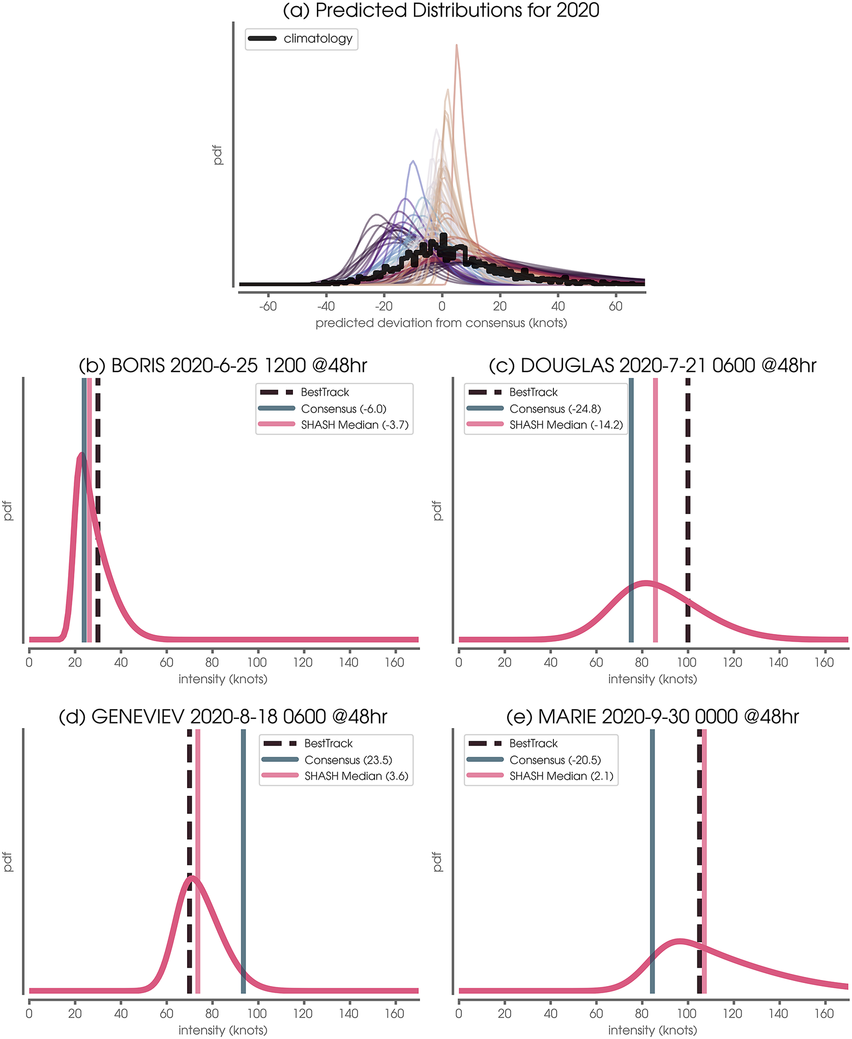
Figure 3. (a) Predicted distributions for testing year 2020. The thick black line denotes the climatological Consensus error distribution across all training and validation samples. (b–e) The example predicted conditional distributions using the SHASH architecture as well as the Best Track verification Consensus forecast. This example is for the Eastern/Central Pacific at 48 hr lead time.
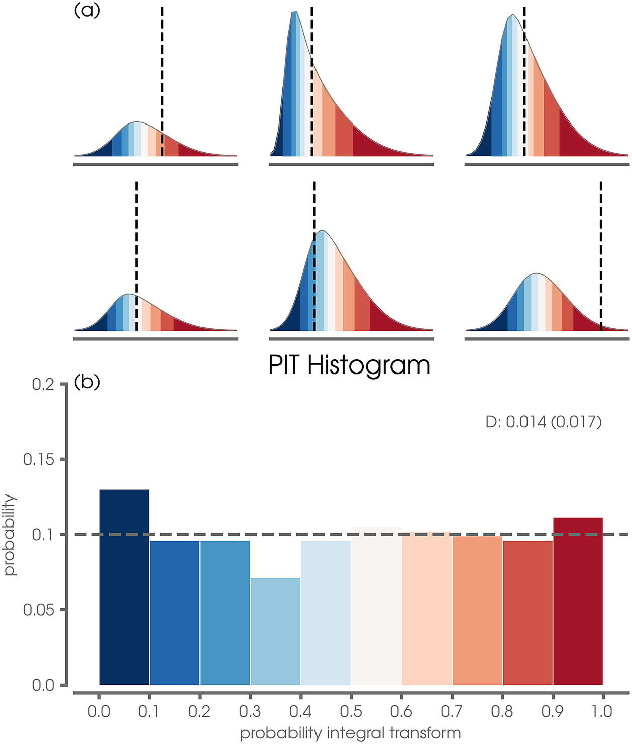
Figure 4. (a) Six example predictions to demonstrate the probability integral transform (PIT) calculation where colored shading denotes different percentile bins in increments of 10%. (b) Final PIT histogram computed for the validation and testing data for the network trained with 2020 as the leave-one-out year. The calibration deviation statistic, $ D $
, is printed in gray; the expected calibration deviation for a perfectly calibrated forecast is given in parentheses. These examples are for the Eastern/Central Pacific at 48 hr lead time.
$ D $
, is printed in gray; the expected calibration deviation for a perfectly calibrated forecast is given in parentheses. These examples are for the Eastern/Central Pacific at 48 hr lead time.
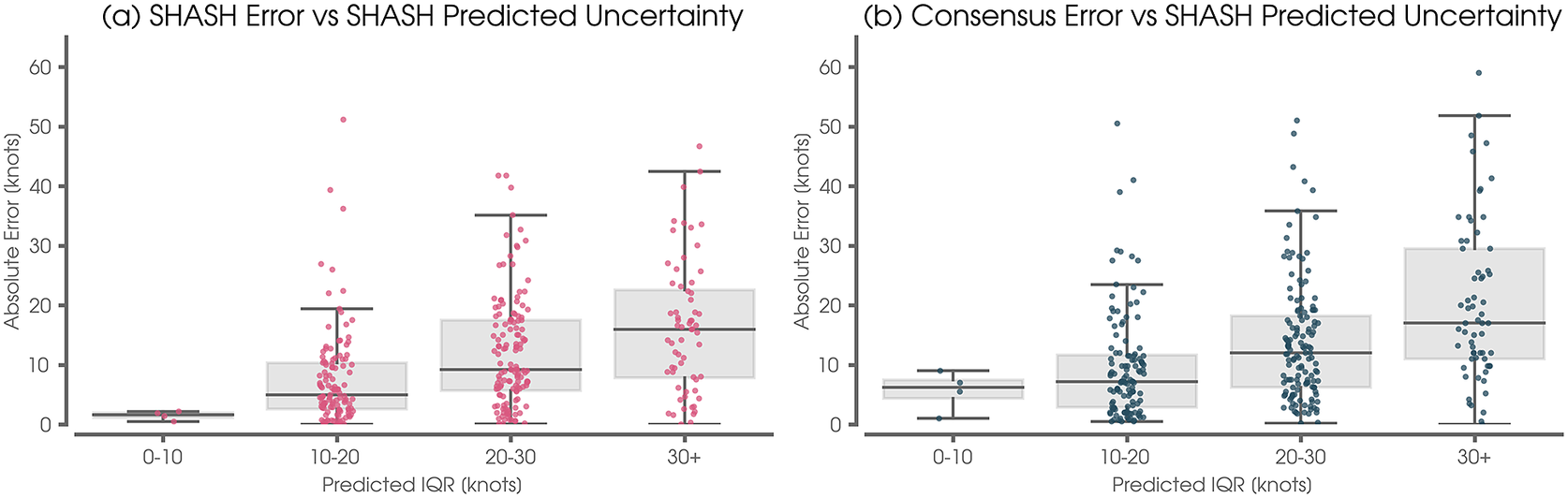
Figure 5. (a) Neural network (NN) mean absolute error versus the network predicted inter-quartile range (IQR). The error is defined as the median of the predicted SHASH distribution minus the Best Track verification. (b) As in (a), but for the Consensus error vs the network-predicted IQR. For both panels, the statistics are computed over the validation and training sets to increase the sample size. This example is for the Eastern/Central Pacific at 48 hr lead time.
4. Alternative uncertainty approaches
4.1. Bayesian neural network
The published research on Bayesian Neural Networks is immense and growing (e.g., Jospin et al., Reference Jospin, Laga, Boussaid, Buntine and Bennamoun2022). Our comparison here is based on vanilla Bayesian Neural Networks for regression as discussed in Duerr et al. (Reference Duerr, Sick and Murina2020) and implemented in TensorFlow 2.7.0. This approach uses Bayes by backprop with Gaussian priors, as defined in Blundell et al. (Reference Blundell, Cornebise, Kavukcuoglu and Wierstra2015), a variational inference approximation, as presented in Graves (Reference Graves2011) (which is built upon the work of Hinton and Camp, Reference Hinton and Camp1993), and computations using the TensorFlow DenseFlipout layers, which are based on Wen et al. (Reference Wen, Vicol, Ba, Tran and Grosse2018).
The BNN architecture and training setup is similar to that of the SHASH approach described in Section 3.2, except it directly draws samples from the posterior predictive distribution of the hurricane intensity errors. In addition, the BNN uses a DenseFlipout layer class to include probabilistic weights and biases that take the form of Gaussian distributions. Otherwise, all other hyperparameters and training approaches remain the same. Unlike the SHASH, however, at inference, the BNN only outputs a single prediction of the Consensus error per one forward pass of a given sample. Thus, to create a BNN-predicted distribution we push each sample through the BNN 5,000 times to create a predicted conditional distribution comparable to the SHASH.
4.2. Monte Carlo Dropout
We additionally present Monte Carlo Dropout (MC Dropout) as a second alternative uncertainty quantification method for comparison. Srivastava et al. (Reference Srivastava, Hinton, Krizhevsky, Sutskever and Salakhutdinov2014) introduced Dropout as a method for reducing the chance of overfitting in neural networks. Specifically, during training, a specific percentage of each layer’s units are temporarily removed (“dropped out”) so that the network must learn to spread predictive information across nodes to make accurate predictions. Dropout is typically only used during training and then turned off during inference. However, it has recently gained traction as a method for uncertainty quantification when left on during inference as well (Gal and Ghahramani, Reference Gal and Ghahramani2015). That is, the MC Dropout method leaves Dropout during inference to obtain a range of predictions for a given sample depending on which units are randomly dropped out.
The MC Dropout architecture and training setup is similar to that of the SHASH approach described in Section 3.2, except (like the BNN) it directly draws samples from the posterior predictive distribution of the hurricane intensity errors. There are additional important differences between the MC Dropout setup and the SHASH and BNN approaches. First, we use a mean absolute error loss function. Next, we train the NN with a dropout rate of 75% in all hidden layers. To that end, we increase the number of units in each layer to have 60 units in the first year and 40 units in the second layer. We note that keeping the number of units the same as in the SHASH and BNN models (i.e., 15 units and 10 units in each layer, respectively) and using a dropout rate of 25% yielded similar conclusions although the MC Dropout model performed more poorly than the architecture presented here (not shown). Finally, we found that a smaller learning rate of 0.00005 was required to train the MC Dropout model. As is the case for the BNN approaches, at inference the MC Dropout approach only outputs a single prediction of the Consensus error per one forward pass of a given sample. Thus, we create an MC Dropout-predicted conditional distribution for each sample by pushing each sample through the network 5,000 times to create a predicted conditional distribution comparable to the SHASH and BNN.
5. Results
We first examine the neural network SHASH predictions for estimating the Consensus error for tropical cyclone intensities over the Eastern/Central Pacific at 48-hr lead times. After discussing a few specific forecasts, we then present multiple evaluation metrics to demonstrate the utility of the SHASH approach. We then end the section with a comparison between the SHASH and two other neural network uncertainty approaches.
5.1. Uncertainty estimation with the SHASH
All predicted SHASH conditional distributions for the Eastern/Central Pacific at a 48-hr lead time and testing year 2020 are plotted in Figure 3a, where the climatological Consensus error distribution of all other years (i.e., training and validation) is shown in black. Although the climatological errors of the Consensus are relatively symmetric about zero, the network predicts a wide range of SHASH distributions. This includes varying location, spread, and skewness depending on the specific 2020 forecast sample. Because the neural network is tasked to predict the Consensus error rather than the intensity itself, negative values denote that the network predicts the Consensus intensity to be too large, and positive values denote that the network predicts the Consensus intensity to be too small.
Four example testing forecast samples are shown in Figure 3b–e. The network’s predicted distribution is plotted in pink, where the Consensus prediction has been added to the predicted SHASH distribution to convert the SHASH to units of tropical cyclone intensity (rather than Consensus intensity error). The vertical dashed line denotes the Best Track verification (i.e., the intensity that actually occurred) and the vertical blue line denotes the Consensus prediction. As already discussed, the network predicts a range of SHASH distributions depending on the specific forecast. For example, the predicted SHASH is heavily positively skewed, but relatively narrow for BORIS (Figure 3b) suggesting that the network is relatively confident in its prediction. The fact that the network places a near-zero probability that BORIS’ intensity will drop below 20 knots is evidence that the network has learned that tropical depressions rarely exhibit intensities less than this, as mentioned in Section 2. In contrast, the network is far less confident in MARIE’s intensity (Figure 3e); subsequently, and so the predicted SHASH exhibits a much wider distribution with a longer positive tail.
A benefit of tasking the network to make a probabilistic forecast is that from this we can produce a range of probabilistic statements about the future tropical cyclone intensity. However, it can at times be helpful to produce a deterministic prediction as well. Here we use the median of the SHASH (shown as a vertical pink line in Figure 3b–e). For all four examples shown here, the median of the SHASH prediction (vertical pink line) is closer to the Best Track verification (vertical dashed line) than the Consensus (vertical blue line), demonstrating that the SHASH can improve the intensity forecast in a deterministic sense and provide a quantification of uncertainty. We present summary metrics of this improvement in the next subsection.
5.2. Evaluation metrics
After training the network, what evidence do we have that our model is any good? On the one hand, one could just compare the true $ y $
value with a deterministic value (i.e., the mean or median of the predicted conditional distribution). However, this type of residual diagnostic does not address whether the predicted uncertainties are useful. While many metrics for evaluating probabilistic predictions exist (e.g., Garg et al., Reference Garg, Rasp and Thuerey2022), here we discuss three.
$ y $
value with a deterministic value (i.e., the mean or median of the predicted conditional distribution). However, this type of residual diagnostic does not address whether the predicted uncertainties are useful. While many metrics for evaluating probabilistic predictions exist (e.g., Garg et al., Reference Garg, Rasp and Thuerey2022), here we discuss three.
The first metric is the simplest. It quantifies the fraction of samples where the true intensity error $ y $
falls between the 25th and 75th percentiles of the predicted SHASH distributions. We call this fraction the “IQR capture fraction.” If the network produces reliable forecasts, then
$ y $
falls between the 25th and 75th percentiles of the predicted SHASH distributions. We call this fraction the “IQR capture fraction.” If the network produces reliable forecasts, then $ y $
should fall within the IQR interval half of the time and the IQR capture fraction should be approximately 0.5. For our SHASH predictions of Eastern/Central Pacific tropical cyclone intensity errors at a 48-hr lead time and 2020 testing year (Figure 6d), the IQR capture fraction is 0.48 over the validation and testing sets (we include validation to increase the sample size for this statistic).
$ y $
should fall within the IQR interval half of the time and the IQR capture fraction should be approximately 0.5. For our SHASH predictions of Eastern/Central Pacific tropical cyclone intensity errors at a 48-hr lead time and 2020 testing year (Figure 6d), the IQR capture fraction is 0.48 over the validation and testing sets (we include validation to increase the sample size for this statistic).
The IQR capture fraction quantifies the fit of predictions that fall in the middle, but what about other percentile combinations? Or the tails of the distribution? Dawid (Reference Dawid1984) introduced the probability integral transform (PIT) as a calibration check for probabilistic forecasts. The PIT works similarly to the IQR capture fraction but is more general. Consider sample $ i $
. Our trained neural network gives us a conditional probability distribution for
$ i $
. Our trained neural network gives us a conditional probability distribution for $ y $
as a function of
$ y $
as a function of $ {x}_i $
. If we denote the cumulative distribution function (CDF) for this conditional distribution
$ {x}_i $
. If we denote the cumulative distribution function (CDF) for this conditional distribution $ F\left(y|{x}_i\right) $
then the probability integral transform (PIT) value for sample
$ F\left(y|{x}_i\right) $
then the probability integral transform (PIT) value for sample $ i $
, which we denote
$ i $
, which we denote $ {p}_i $
, is
$ {p}_i $
, is
 $$ {p}_i=F\left({y}_i|{x}_i\right). $$
As explained in Gneiting and Katzfuss (Reference Gneiting and Katzfuss2014), $ {p}_i $
is the predicted CDF evaluated during the observation. Six such example calculations of
$ {p}_i $
is the predicted CDF evaluated during the observation. Six such example calculations of $ {p}_i $
are shown in Figure 4a. The histogram of all such values over the data set is called the PIT histogram (Figure 4b). If the predictive model is ideal, then the PIT histogram follows a uniform distribution (Gneiting et al., Reference Gneiting, Balabdaoui and Raftery2007).
$ {p}_i $
are shown in Figure 4a. The histogram of all such values over the data set is called the PIT histogram (Figure 4b). If the predictive model is ideal, then the PIT histogram follows a uniform distribution (Gneiting et al., Reference Gneiting, Balabdaoui and Raftery2007).
Figure 4b shows the PIT histogram for the validation and testing samples for the Eastern/Central Pacific predictions at a 48-hr lead time for testing year 2020. The validation data are included to increase sample size, since the PIT histogram becomes meaningless when the evaluation set is too small (Hamill, Reference Hamill2001; Bourdin et al., Reference Bourdin, Nipen and Stull2014). A perfectly calibrated forecast is expected to have a PIT histogram that is uniform distribution (that is flat). As seen in Figure 4b, the predicted PIT histogram is nearly uniform. Following Nipen and Stull (Reference Nipen and Stull2011) and Bourdin et al. (Reference Bourdin, Nipen and Stull2014), we compute the PIT $ D $
statistic to quantify the degree of deviation from a flat PIT histogram:
$ D $
statistic to quantify the degree of deviation from a flat PIT histogram:
 $$ D=\sqrt{\frac{1}{B}\sum \limits_{k=1}^B{\left({b}_k-\frac{1}{B}\right)}^2}, $$
where $ k $
is an integer denoting the bin number that ranges from 1 to the total number of bins
$ k $
is an integer denoting the bin number that ranges from 1 to the total number of bins $ B $
and
$ B $
and $ {b}_k $
denotes the bin frequency of the
$ {b}_k $
denotes the bin frequency of the $ k $
th bin. For our case,
$ k $
th bin. For our case, $ B=10 $
and
$ B=10 $
and $ D=0.014 $
. Again following Bourdin et al. (Reference Bourdin, Nipen and Stull2014), a perfectly calibrated forecast will produce a PIT histogram that is perfectly flat. The expected deviation is given by
$ D=0.014 $
. Again following Bourdin et al. (Reference Bourdin, Nipen and Stull2014), a perfectly calibrated forecast will produce a PIT histogram that is perfectly flat. The expected deviation is given by
 $$ E\left[{D}_p\right]=\sqrt{\frac{1-{B}^{-1}}{TB}}, $$
where $ {D}_p $
denotes the PIT
$ {D}_p $
denotes the PIT $ D $
statistic for a perfectly calibrated forecast and
$ D $
statistic for a perfectly calibrated forecast and $ T $
is the total number of samples over which the PIT was computed. For our case, this expected deviation is
$ T $
is the total number of samples over which the PIT was computed. For our case, this expected deviation is $ E\left[{D}_p\right]=0.017 $
. The computed
$ E\left[{D}_p\right]=0.017 $
. The computed $ D $
for the PIT histogram shown in Figure 4b is
$ D $
for the PIT histogram shown in Figure 4b is $ D=0.014 $
, and so, it cannot be distinguished from that produced by a perfectly calibrated forecast. We will make use of the PIT
$ D=0.014 $
, and so, it cannot be distinguished from that produced by a perfectly calibrated forecast. We will make use of the PIT $ D $
statistics to summarize the calibration of all networks later in this section.
$ D $
statistics to summarize the calibration of all networks later in this section.
An additional way to visualize the utility of the network’s probabilistic forecast is to assess the extent to which a wider predicted SHASH relates to larger errors using the median as a deterministic prediction. Put another way, when the SHASH distribution is narrow, we would like the median of the predicted SHASH to be closer to the truth than when the SHASH distribution is wide. We quantify the width of the SHASH using the interquartile range (IQR) and plot the NN’s deterministic error against this predicted IQR in Figure 5a. Indeed, we see a strong correlation between the network’s deterministic error and the IQR of the predicted SHASH, demonstrating that the width of the predicted distribution can be used as a measure of uncertainty. Furthermore, Figure 5b shows that the IQR of the predicted SHASH also correlates with the Consensus prediction error. That is, the width of the predicted SHASH can be used as a metric to assess uncertainty in the Consensus forecast itself.
Equipped with multiple metrics to evaluate the NN’s SHASH prediction, Figure 6 summarizes the deterministic errors (Figure 6a) and the three probabilistic metrics (Figure 6b–d) across all nine leave-one-out testing years for a range of lead times and ocean basins (x-axis). Our results show that the deterministic NN forecast (based on the median of the predicted SHASH) can improve upon the Consensus forecast at shorter lead times in both basins, but struggles to improve upon the Consensus at 96- and 120-hr lead times (Figure 6a).
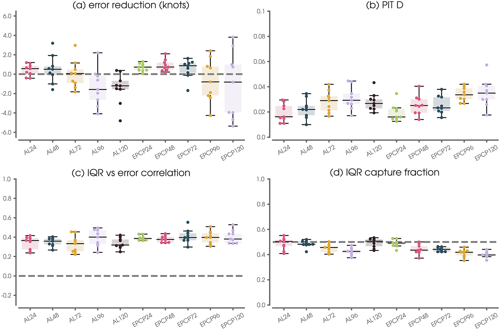
Figure 6. SHASH performance metrics across a range of basins and lead times for each of the nine leave-one-out testing years (denoted by dots). The x-axis label convention is such that AL denotes the Atlantic basin and EPCP denotes the combined Eastern and Central Pacific basins. Numbers denote the forecast lead time in hours. Panel (a) shows testing results only, while panels (b)–(d) show results over validation and testing sets to increase the sample size for the computed statistics. See the text for details on the calculation of each metric.
Even in the event that the NN does not improve upon the Consensus forecast in a deterministic sense, Figure 6b–d demonstrates that the SHASH predictions provide useful uncertainty quantifications. The PIT $ D $
statistics show small values (Figure 6b) and the IQR capture fractions fall near 0.5 (Figure 6d). Figure 6c summarizes results of the comparison shown in Figure 5a by displaying the Spearman rank correlation between the NN absolute error (based on the median) and the predicted IQR. For context, the example shown in Figure 5a exhibits a Spearman correlation of 0.5. Thus, we see that for all combinations of lead time and basin, the NN-SHASH provides a meaningful measure of uncertainty that correlates with the deterministic error.
$ D $
statistics show small values (Figure 6b) and the IQR capture fractions fall near 0.5 (Figure 6d). Figure 6c summarizes results of the comparison shown in Figure 5a by displaying the Spearman rank correlation between the NN absolute error (based on the median) and the predicted IQR. For context, the example shown in Figure 5a exhibits a Spearman correlation of 0.5. Thus, we see that for all combinations of lead time and basin, the NN-SHASH provides a meaningful measure of uncertainty that correlates with the deterministic error.
5.2. SHASH applications to rapid intensification probabilities
Although NHC’s intensity forecast skill has shown significant improvement over the last decade (Cangialosi et al., Reference Cangialosi, Blake, DeMaria, Penny, Latto, Rappaport and Tallapragada2020), there has been less progress in the ability forecast rapid intensification (RI) (DeMaria et al., Reference DeMaria, Franklin, Onderlinde and Kaplan2021). As described by Kaplan (Reference Kaplan2015), there are a number of definitions of RI, but the most common ones are intensity increases of 30 knots or greater in 24 hr, 55 knots or greater in 48 hr, and 65 knots in 72 hr. As shown by DeMaria et al. (Reference DeMaria, Franklin, Onderlinde and Kaplan2021), dynamical models such as HWRF and HMON have shown some ability to forecast RI in the past few years. However, the most accurate guidance is based on statistical methods such as linear discriminate analysis or logistic regression, where RI is treated as a classification problem.
Because the NN-SHASH provides complete error distribution, it can be used to provide RI guidance. We further demonstrate the benefits of the NN-SHASH approach by using the predicted conditional SHASH distribution to quantify the probability of tropical cyclone rapid intensification (RI). Here, we use the predicted SHASH to forecast the probability of RI occurrence. An example of this is shown in Figure 7a for the Atlantic 48-hr forecast for Hurricane Michael on October 10, 2018. The intensity at the time of forecast (50 knots) is shown by the vertical gray line and the predicted intensity distribution at 48 hr is denoted by the pink curve. By definition, RI requires an increase of 55 knots over a 48-hr period, which corresponds to an intensity of $ 50+55=105 $
knots. Thus, by integrating under the predicted SHASH distribution from 105 knots and above, we obtain a predicted probability of RI of 47%. In fact, Michael did undergo RI during this time, increasing its intensity over 48 hr by 60 knots to 110 knots (dashed black line).
$ 50+55=105 $
knots. Thus, by integrating under the predicted SHASH distribution from 105 knots and above, we obtain a predicted probability of RI of 47%. In fact, Michael did undergo RI during this time, increasing its intensity over 48 hr by 60 knots to 110 knots (dashed black line).
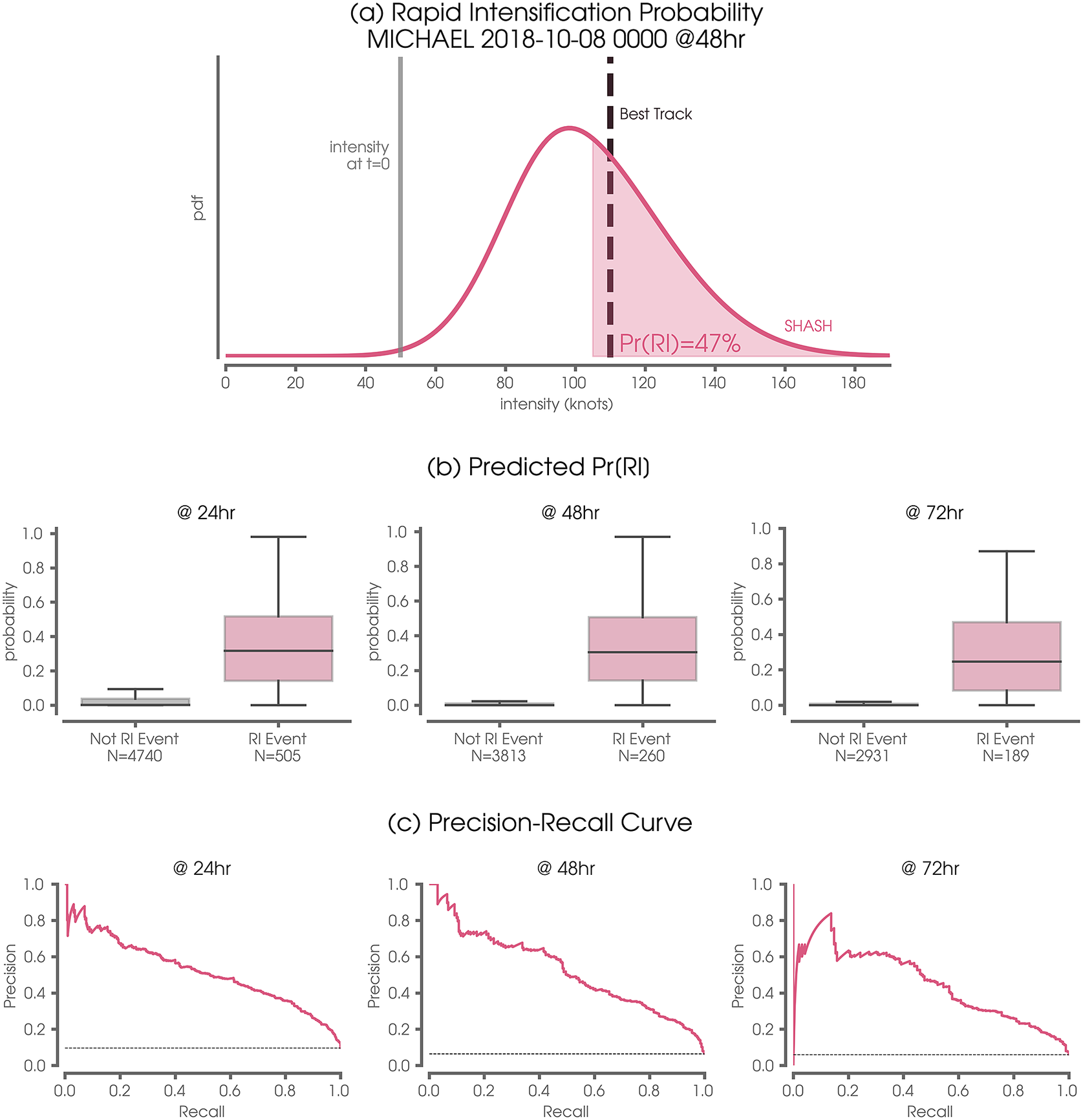
Figure 7. (a) Example case study demonstrating the utility of the SHASH for predicting the probability of rapid intensification (Pr(RI); pink shading). The pink curve denotes the predicted conditional distribution by the SHASH at 48-hr lead time for Hurricane Michael on October 8, 2018. The gray vertical line denotes the storm intensity at the time of the forecast and the vertical dashed line denotes the Best Track verification. (b) Predicted probability of rapid intensification at various lead times for all East/Central Pacific and Atlantic storms for all nine leave-one-out testing years. The gray box plot denotes predicted probabilities for storms that did not undergo rapid intensification, while the pink box plot denotes predicted probabilities for storms that did. (c) As in (b), but the precision-recall curves for RI as a function of lead time. The dashed black line denotes the baseline precision in the case of no skill.
We compute the probability of RI over all predictions for the Atlantic and Eastern/Central Pacific for all nine leave-one-out testing years and group the results by whether or not RI actually occurred (Figure 7b). For nearly all cases that undergo RI (pink boxes), the NN predicts a non-zero probability of RI. Contrast this with cases that do not undergo RI (gray boxes), where nearly all cases exhibit a near-zero predicted probability. The Mann–Whitney U statistic comparing the distributions in each panel of Figure 7 result in p-values of $ 2\mathrm{e}-194 $
,
$ 2\mathrm{e}-194 $
, $ 4\mathrm{e}-117 $
, and
$ 4\mathrm{e}-117 $
, and $ 3\mathrm{e}-80 $
for the three panels in Figure 7b, respectively. Thus, the NN approach is clearly able to distinguish between cases that will likely undergo RI and those that will not. The precision-recall curves shown in Figure 7c further demonstrate that the NN has skill in predicting RI at all three lead times. While a more thorough analysis is required to quantify the extent to which our RI predictions improve upon current operational methods, our focus here is to demonstrate the potential utility of the approach.
$ 3\mathrm{e}-80 $
for the three panels in Figure 7b, respectively. Thus, the NN approach is clearly able to distinguish between cases that will likely undergo RI and those that will not. The precision-recall curves shown in Figure 7c further demonstrate that the NN has skill in predicting RI at all three lead times. While a more thorough analysis is required to quantify the extent to which our RI predictions improve upon current operational methods, our focus here is to demonstrate the potential utility of the approach.
Taking our analysis one step further, we utilize AI explainability methods (e.g., McGovern et al., Reference McGovern, Lagerquist, Gagne, Jergensen, Elmore, Homeyer and Smith2019; Mamalakis et al., Reference Mamalakis, Ebert-Uphoff and Barnes2022) to better understand why the NN predicted the distribution that it did. For example, we can further explore the high predicted probability of RI by plotting the gradient of the output with respect to the input features of the NN for the 48-hr prediction of Michael on October 10, 2018. Since the gradient is computed for each output separately, we obtain a measure of the sensitivity of the predicted SHASH parameters to small increases in each of the 12 features (Figure 8a). Based on this gradient calculation, the NN would have predicted smaller parameters if the storm had been slightly further north (i.e., more positive SLAT). Furthermore, had the Consensus (VMXC) been slightly larger, the NN would also have predicted larger SHASH parameters. Interestingly, the NN appears more sensitive to the LGEM forecast than the others for this particular prediction, suggesting that had the LGEM forecast been larger the NN would have increased its predicted parameters as well. We repeated this analysis for Hurricane Marie for the same case shown in Figure 3e, and the results are plotted in Figure 8b. Unlike for Hurricane Michael, had the Consensus (VMXC) been slightly larger, the NN would have predicted larger $ \mu $
but smaller
$ \mu $
but smaller $ \sigma $
. Furthermore, had the intensity at the time of forecast (VMAX0) been slightly larger, the NN would have also increased its
$ \sigma $
. Furthermore, had the intensity at the time of forecast (VMAX0) been slightly larger, the NN would have also increased its $ \mu $
and decreased
$ \mu $
and decreased $ \sigma $
. This suggests that explainability methods can be used to understand differences in the NN’s decision-making process for specific forecasts. We leave the exploration of additional case studies and explainability methods for future work.
$ \sigma $
. This suggests that explainability methods can be used to understand differences in the NN’s decision-making process for specific forecasts. We leave the exploration of additional case studies and explainability methods for future work.
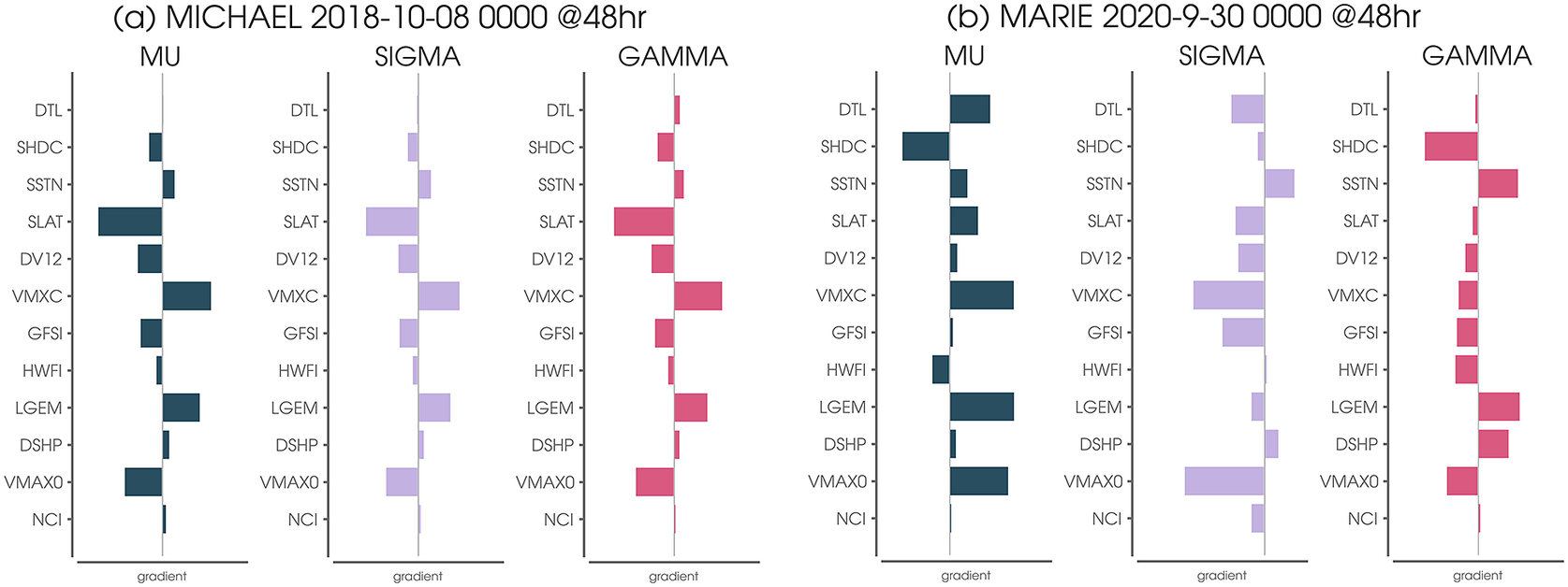
Figure 8. (a) Neural network gradient for the 48-hr SHASH prediction for Hurricane Michael on October 8, 2018. The gradient describes how small increases in each input predictor would have changed the prediction of each of the three SHASH parameters (the tailweight $ \tau $
is fixed to 1.0). (b) As in (a), but for Hurricane Marie on September 30, 2020.
$ \tau $
is fixed to 1.0). (b) As in (a), but for Hurricane Marie on September 30, 2020.
5.3. Comparison with alternative neural network uncertainty approaches
It is worth briefly contrasting the SHASH approach discussed here with that of other approaches such as Monte Carlo Dropout (MC Dropout) and Bayesian neural networks (BNN) that have become go-to methods for incorporating uncertainty into artificial neural networks (e.g., Wilson, Reference Wilson2020; Foster et al., Reference Foster, Gagne and Whitt2021). While both MC Dropout and BNN architectures can vary greatly in detail, we focus here on a simple implementation of each. Our aim is not to provide an exhaustive comparison, nor to claim that one method is the “winner” over the others but, rather, to provide a comparison between the methods using the same problem setup and data. Furthermore, our aim is not to review, compare, or summarize the hundreds (perhaps thousands) of species and subspecies of uncertainty quantification present in the machine learning ecosystem (see, e.g., Abdar et al., Reference Abdar, Pourpanah, Hussain, Rezazadegan, Liu, Ghavamzadeh, Fieguth, Cao, Khosravi, Acharya, Makarenkov and Nahavandi2021; Jospin et al., Reference Jospin, Laga, Boussaid, Buntine and Bennamoun2022). Instead, we implement BNNs and MC Dropout using the default configurations provided by TensorFlow 2.7.0 (https://www.tensorflow.org/) and its TensorFlow Probability 0.15.0 package (https://www.tensorflow.org/probability) as a scientist might when trying to determine which method to explore further.
Predictions for the four use cases discussed in Section 5.2 are shown in Figure 9, but now compare the three uncertainty quantification approaches (see Section 4 for details; SHASH predictions are identical to those in Figure 2b–d). While all three approaches produce predicted conditional distributions, MC Dropout tends to produce distributions that are much narrower than the other two methods and the BNN-predicted distributions tend to be more symmetric. This is particularly evident for BORIS (Figure 9a), where the BNN predicts non-zero probabilities of 0 knot intensities.
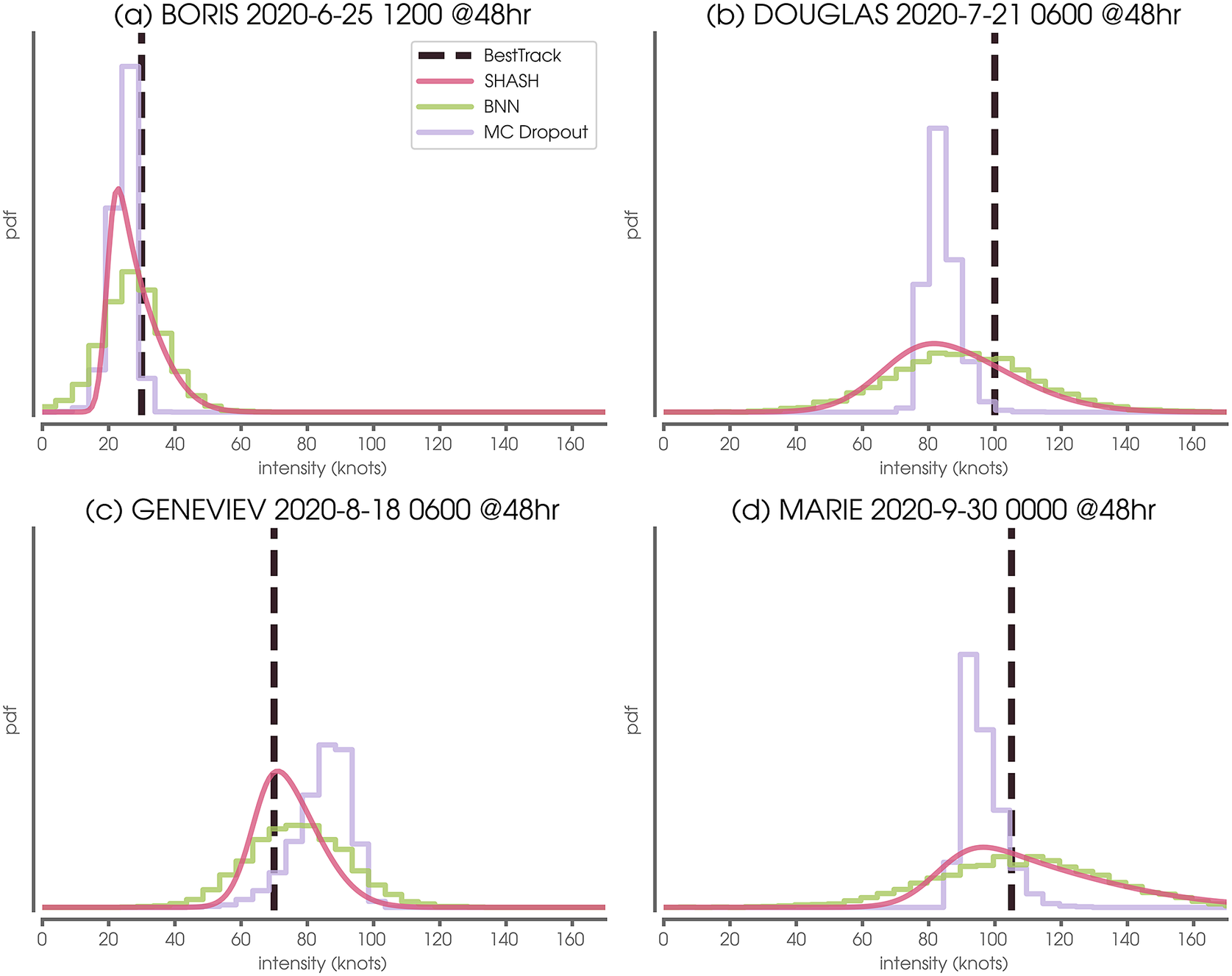
Figure 9. Example conditional distributions predicted by four neural network probabilistic methods. Vertical dashed line denotes the Best Track verification.
Figure 10 shows summary metrics across all nine leave-one-out testing years as in Figure 6 but compare the three different approaches for estimating uncertainty. While all three approaches are similarly able to reduce the Consensus prediction error in a deterministic sense, panels (b)–(d) show that their probabilistic properties differ. MC Dropout tends to produce distributions that are much too narrow. This is quantified by the large PIT $ D $
statistics (Figure 10b), a lack of strong correlation between the IQR and deterministic error (Figure 10c), and IQR capture fractions far below 0.5 (Figure 10d). This failure of MC Dropout was also noted by Garg et al. (Reference Garg, Rasp and Thuerey2022) for medium-range weather forecasts. The BNN performs much more similar to the simple SHASH, and in some cases may even perform better, although only marginally so. Trade-offs between the SHASH and BNN approaches will be discussed further in Section 6.
$ D $
statistics (Figure 10b), a lack of strong correlation between the IQR and deterministic error (Figure 10c), and IQR capture fractions far below 0.5 (Figure 10d). This failure of MC Dropout was also noted by Garg et al. (Reference Garg, Rasp and Thuerey2022) for medium-range weather forecasts. The BNN performs much more similar to the simple SHASH, and in some cases may even perform better, although only marginally so. Trade-offs between the SHASH and BNN approaches will be discussed further in Section 6.
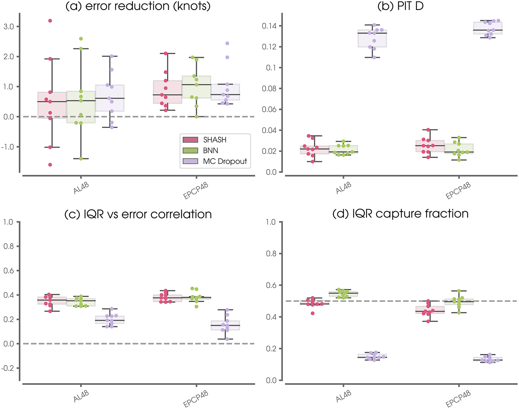
Figure 10. As in Figure 6, but for the SHASH, BNN, and MC-Dropout approaches for Atlantic (AL) and Pacific (EPCP) forecasts at 48-hr lead times for all nine leave-one-out testing years.
6. Discussion
Here, we present a simple method that estimates the conditional distribution for each sample. It was originally proposed by Nix and Weigend (Reference Nix and Weigend1994) and has been presented as a standard approach in recent literature, for example, Duerr et al. (Reference Duerr, Sick and Murina2020), the TensorFlow manual, and many data science blogs. Even so, it appears relatively unknown in the earth science community. The approach is simple, can be applied to most any network architecture, and can be adapted to different uncertainty distributions via the choice of the underlying distribution. Here, we explore the family of sinh-arcsinh-normal (SHASH) distributions (Jones and Pewsey, Reference Jones and Pewsey2009) as a general set that can capture location, spread, and skewness of the posterior distribution in an intuitive manner. However, we note that other distributions (e.g., the lognormal distribution) may be better choices for specific applications.
In addition to be being straightforward to understand and implement, the NN-SHASH approach is computationally efficient, especially at inference. For example, on a late 2019 iMac with six cores and 32 GB of RAM, the NN-SHASH took 5 s to predict distributions for 124 testing samples. In contrast, MC Dropout took 9 s to predict the distributions using 5,000 draws each, and the BNN took 163 s to predict the distributions using 5,000 draws each. Thus, although the BNN performs similarly to the NN-SHASH, it is more computationally expensive at inference and significantly more difficult to understand given the complexities of the variational inference method employed during training.
Our SHASH approach aims to quantify the predictive uncertainty, being agnostic to whether the uncertainty comes from the data noise or from the model itself. The SHASH model presented here uses a maximum likelihood approach to estimate the parameters of the SHASH distribution, and does not explicitly quantify, or account for, errors in the learned SHASH parameters. Thus, the proposed approach does not account for errors in the learned parameters (and could underestimate the true predictive uncertainty) when either the SHASH distribution provides a poor approximation to the true predictive distribution or when the SHASH parameter estimates are inaccurate. For example, this may occur when there is too little training data in the neighborhood of the input. With that said, our leave-one-out (year by year) analysis captures uncertainties in the learned SHASH parameters via training nine separate networks (see Figures 6 and 10).
Finally, we note that while TensorFlow provides an implementation of the family of sinh-arcsinh distributions, it does not provide certain SHASH metrics (e.g., mean, standard deviation, and variance) at the time of publication of this work. We have provided documentation in Appendix B of how we have implemented these metrics for the sinh-arcsinh-normal distribution. We also provide code to fill this gap.
7. Conclusions
Estimating the parameters of a sinh-arcsinh-normal probability distribution function is a simple, straightforward method for adding uncertainty to neural network regression tasks. The method provides reliable uncertainty estimates when applied to predictions of tropical cyclone intensity errors. The authors believe it will become a powerful, go-to method moving forward.
Author contribution
Conceptualization: E.A.B., R.J.B., M.D.; Data curation: M.D.; Data visualisation: E.A.B.; Methodology: E.A.B., R.J.B.; Writing—original draft: E.A.B., R.J.B., M.D. All authors approved the final submitted draft.
Competing interest
The authors declare none.
Data availability statement
Atlantic, eastern North Pacific, and central North Pacific operational model and best track data were obtained from the National Hurricane Center. The code and data set prepared for this work can be found on Zenodo at the following permanent DOI: https://doi.org/10.5281/zenodo.7915589.
Ethics statement
The research meets all ethical guidelines, including adherence to the legal requirements of the study country.
Funding statement
This research was supported, in part, by a National Science Foundation CAREER Award AGS-1749261 and the National Science Foundation AI Institute for Research on Trustworthy AI in Weather, Climate, and Coastal Oceanography (AI2ES) under NSF grant ICER-2019758.
A. Appendix A
A.1. Sample sizes
Table of sample sizes for each basin and lead time for leave-one-out testing year 2020. AL denotes the Atlantic basin and EPCP denotes the Eastern/Central Pacific basin.
B. Appendix B
B.1. Sinh-arcsinh-Normal Formulations
B.1.1. Jones and Pewsey Formulation
B.1.1.1. Notation
The sinh-arcsinh-normal distribution was defined by Jones and Pewsey (Reference Jones and Pewsey2009). A more accessible, though less complete, presentation is given by Jones and Pewsey (Reference Jones and Pewsey2019). The following notation, which is used in this Appendix, is from the later paper:
-
• location $ \xi \in \mathrm{\mathbb{R}} $
,
$ \xi \in \mathrm{\mathbb{R}} $
, -
• scale
$ \eta >0 $
, -
• skewness
$ \varepsilon \in \mathrm{\mathbb{R}} $
, -
• tailweight
$ \delta >0 $
.


B.1.1.2. Distribution
Following Jones and Pewsey (Reference Jones and Pewsey2019), the sinh-arcsinh transformation of a random variable $ \chi $
is defined as
$ \chi $
is defined as
 $$ S\left(\chi; \alpha, \beta \right)=\sinh \left(\beta \cdot \mathrm{asinh}\left(\chi \right)-\alpha \right). $$
A sinh-arcsinh-normal random variable $ X $
is defined as
$ X $
is defined as
 $$ X=\xi +\eta \cdot S\left(Z;\unicode{x025B}, \delta \right), $$
where $ Z $
is a standard normal random variable. The probability density function of
$ Z $
is a standard normal random variable. The probability density function of $ X $
is
$ X $
is
 $$ f(x)=\frac{\delta }{\eta}\cdot \sqrt{\frac{1+{S}^2\left(y;\unicode{x025B}, \delta \right)}{2\pi \left(1+{y}^2\right)}}\cdot \exp \left(-\frac{1}{2}{S}^2\left(y;\unicode{x025B}, \delta \right)\right), $$
where
 $$ y=\frac{x-\xi }{\eta }. $$
B.1.1.3. Moments
The first three moments of $ S=S\left(Z;\unicode{x025B}, \delta \right) $
are derived in Jones and Pewsey (Reference Jones and Pewsey2009, p. 764) as
$ S=S\left(Z;\unicode{x025B}, \delta \right) $
are derived in Jones and Pewsey (Reference Jones and Pewsey2009, p. 764) as
 $$ \boldsymbol{E}(S)=\sinh \left(\unicode{x025B} /\delta \right)\cdot {P}_{1/\delta }, $$
 $$ \boldsymbol{E}\left({S}^2\right)=\frac{1}{2}\left[\cosh \left(2\unicode{x025B} /\delta \right)\cdot {P}_{2/\delta }-1\right], $$
 $$ \boldsymbol{E}\left({S}^3\right)=\frac{1}{4}\left[\sinh \left(3\unicode{x025B} /\delta \right)\cdot {P}_{3/\delta }-3\sinh \left(\unicode{x025B} /\delta \right)\cdot {P}_{1/\delta}\right], $$
where
 $$ {P}_q=\frac{e^{1/4}}{\sqrt{8\pi }}\cdot \left[{K}_{\left(q+1\right)/2}\left(1/4\right)+{K}_{\left(q-1\right)/2}\left(1/4\right)\right] $$
and $ K $
is the modified Bessel function of the second kind.
$ K $
is the modified Bessel function of the second kind.
B.1.1.4. Descriptive statistics
We compute the mean of $ X $
as
$ X $
as
 $$ \boldsymbol{E}(X)=\boldsymbol{E}\left(\xi +\eta \cdot S\right) $$
 $$ =\xi +\eta \cdot \boldsymbol{E}(S). $$
We compute the variance of $ X $
as
$ X $
as
 $$ \boldsymbol{Var}(X)=\boldsymbol{Var}\left(\xi +\eta \cdot S\right) $$
 $$ ={\eta}^2\cdot \boldsymbol{Var}(S) $$
 $$ ={\eta}^2\cdot \left[\boldsymbol{E}\left({S}^2\right)-\boldsymbol{E}{(S)}^2\right]. $$
We compute the skewness of $ X $
(also known as the third standardized moment) as
$ X $
(also known as the third standardized moment) as
 $$ \boldsymbol{Skew}(X)=\frac{\boldsymbol{E}\left({X}^3\right)-3\boldsymbol{E}(X)\boldsymbol{Var}(X)-\boldsymbol{E}{(X)}^3}{\boldsymbol{Var}{(X)}^{\left(3/2\right)}}. $$
Wikipedia contributors (2022), where
 $$ \boldsymbol{E}\left({X}^3\right)={\xi}^3+3{\xi}^2\eta \boldsymbol{E}(S)+3{\xi \eta}^2\boldsymbol{E}\left({S}^2\right)+{\eta}^3\boldsymbol{E}\left({S}^3\right), $$
Beware: in general, $ \boldsymbol{E}(X)\ne \xi $
,
$ \boldsymbol{E}(X)\ne \xi $
, $ \boldsymbol{Var}(X)\ne {\eta}^2 $
, and
$ \boldsymbol{Var}(X)\ne {\eta}^2 $
, and $ \boldsymbol{Skew}(X)\ne \unicode{x025B} $
.
$ \boldsymbol{Skew}(X)\ne \unicode{x025B} $
.
B.2. TensorFlow Formulation
B.2.1. Notation
TensorFlow includes the sinh-arcsinh-normal distribution as the default case of a more general family of transformed distributions implemented in the tfp.distributions package as SinhArcsinh. The notation used in TensorFlow is similar to the notation used by Jones and Pewsey, but the two are not identical:
-
• loc
$ \in \mathrm{\mathbb{R}} $
, -
• scale
$ >0 $
, -
• skewness
$ \in \mathrm{\mathbb{R}} $
, -
• tailweight
$ >0 $
.


Specifically, the words used by Jones and Pewsey are the same as the words used by TensorFlow, but the meanings of scale and tailweight are different. More on this below.
B.2.2. Distribution
TensorFlow defines the sinh-arcsinh-normal distribution somewhat differently than Jones and Pewsey. A sinh-arcsinh-normal random variable $ Y $
is defined as
$ Y $
is defined as
 $$ Y=\mathtt{loc}+\mathtt{scale}\cdot F(Z). $$
where
 $$ F(Z)=\sinh \left(\left[\mathrm{asinh}(Z)+\mathtt{skewness}\right]\cdot \mathtt{tailweight}\right)\cdot \frac{2}{F_0(2)} $$
and
 $$ {F}_0(2)=\sinh \left(\mathrm{asinh}(2)\cdot \mathtt{tailweight}\right). $$
We compare (A.1) and (A.2) to (A.16), (A.17), and (A.18) to see that the two formulations are equivalent—that is, $ X $
and
$ X $
and $ Y $
are equivalent random variables—if
$ Y $
are equivalent random variables—if
 $$ \xi =\mathtt{loc}, $$
 $$ \eta =\mathtt{scale}\cdot \frac{2}{F_0(2)}, $$
 $$ \unicode{x025B} =\mathtt{skewness}, $$
 $$ \delta =\frac{1}{\mathtt{tailweight}}. $$
We note the likely source of confusion due to the descriptor “tailweight”. In Jones and Pewsey (Reference Jones and Pewsey2009), $ \delta $
is said to “control the tailweight”, and in Jones and Pewsey (Reference Jones and Pewsey2019),
$ \delta $
is said to “control the tailweight”, and in Jones and Pewsey (Reference Jones and Pewsey2019), $ \delta $
is called the “tail weight parameter”. Nonetheless,
$ \delta $
is called the “tail weight parameter”. Nonetheless, $ \delta $
is the reciprocal of the tailweight in TensorFlow.
$ \delta $
is the reciprocal of the tailweight in TensorFlow.
B.3. Implementation
We substitute (A.21) and (A.22) into (A.5), (A.6), and (A.7) to compute the first three moments of $ S $
. The only modifications are
$ S $
. The only modifications are
 $$ \unicode{x025B} /\delta =\mathtt{skewness}\cdot \mathtt{tailweight} $$
and
 $$ i/\delta =i\cdot \mathtt{tailweight} $$
where $ i\in \left\{\mathrm{1,2,3}\right\} $
. We compute the mean, variance, and skewness of
$ i\in \left\{\mathrm{1,2,3}\right\} $
. We compute the mean, variance, and skewness of $ Y $
using (A.10), (A.13), (A.14), and (A.15) by first computingFootnote 1
$ Y $
using (A.10), (A.13), (A.14), and (A.15) by first computingFootnote 1
 $$ \eta =\mathtt{scale}\cdot \frac{2}{\sinh \left(\mathrm{asinh}(2)\cdot \mathtt{tailweight}\right)} $$
and setting $ \xi =\mathtt{loc} $
.
$ \xi =\mathtt{loc} $
.
B.4. Notation in this paper
As our neural network implementation is based on TensorFlow, we follow the TensorFlow nomenclature in the body of this paper. For brevity, we introduce the following notation:
-
•
$ \mu =\mathtt{loc} $
, -
•
$ \sigma =\mathtt{scale} $
, -
•
$ \gamma =\mathtt{skewness} $
, -
•
$ \tau =\mathtt{tailweight} $
.


Note: in general, $ \boldsymbol{E}(Y)\ne \mu $
,
$ \boldsymbol{E}(Y)\ne \mu $
, $ \boldsymbol{Var}(Y)\ne {\sigma}^2 $
, and
$ \boldsymbol{Var}(Y)\ne {\sigma}^2 $
, and $ \boldsymbol{Skew}(Y)\ne \gamma $
.
$ \boldsymbol{Skew}(Y)\ne \gamma $
.


 Open access