


1. INTRODUCTION
Receiver Autonomous Integrity Monitoring (RAIM) (Lee, Reference Lee1986; Parkinson and Axelrad, Reference Parkinson and Axelrad1988) is implemented in Global Navigation Satellite Systems (GNSS) to protect users against potential integrity threats caused, for example, by satellite failures. RAIM not only aims at detecting faults but also at evaluating the integrity risk, which is the probability of undetected faults causing unacceptably large errors in the estimated position (RTCA Special Committee 159, 2004). Hence, both the detector and the estimator influence RAIM performance. This two-part research work describes the design, analysis and evaluation of new methods to determine the optimal detector and estimator, which minimize the integrity risk in RAIM. Part 1 focused on optimal detection methods (Joerger et al., Reference Joerger, Stevanovic, Langel and Pervan2015). Part 2 is presented in this paper, and addresses estimator design for integrity risk minimisation.
The core principle of RAIM is to exploit redundant measurements to achieve self-contained fault detection at the user receiver. With the modernisation of the Global Positioning System (GPS), the full deployment of GLONASS, and the emergence of Galileo and BeiDou, an increased number of redundant ranging signals becomes available, which has recently drawn a renewed interest in RAIM. In particular, RAIM can help alleviate requirements on ground monitors. For example, researchers in the European Union and in the United States are investigating Advanced RAIM (ARAIM) for worldwide vertical guidance of aircraft (EU-US Cooperation on Satellite Navigation, 2012).
One of the primary tasks in RAIM is to evaluate the integrity risk, or alternatively, a protection level, which is an integrity bound on the positioning error. Integrity risk evaluation is needed when designing a navigation system to meet predefined integrity requirements, and it is needed operationally to inform the user whether to abort or to pursue a mission. Integrity risk evaluation involves both assessing the fault-detection capability and quantifying the impact of undetected faults on position estimation errors.
Both the RAIM detector and the estimator have been investigated in the literature. With regard to fault detection, multiple RAIM algorithms have been devised and implemented over the past 25 years, including Solution Separation (SS) RAIM (Brenner, Reference Brenner1996; Blanch et al., Reference Blanch, Ene, Walter and Enge2007). In parallel, with regard to estimation, researchers have explored the potential of replacing the conventional Least-Squares (LS) process with a Non-Least-Squares (NLS) estimator to lower the integrity risk in exchange for a slight increase in nominal positioning error (Hwang and Brown, Reference Hwang and Brown2006; Lee, Reference Lee2008; Blanch et al., Reference Blanch, Walter and Enge2012). The resulting methods show promising reductions in integrity risk, but are computationally expensive for real-time implementations.
In response, this two-part research effort provides new methods to determine the optimal detector and estimator in RAIM, which minimise integrity risk. Optimal design of the detector and of the estimator is respectively tackled in Part 1 (i.e., in Joerger et al. (Reference Joerger, Stevanovic, Langel and Pervan2015)) and in Part 2 (i.e., in this paper). Of particular concern is the fact that the new methods may be implemented in applications where processing resources are limited. In this perspective, computationally-efficient, near-optimal algorithms are developed, and the trade-off between increasing computation time and decreasing integrity risk is quantified.
The detectors in RAIM were analysed in Part 1 using parity space representations (Joerger et al., Reference Joerger, Stevanovic, Langel and Pervan2015). The parity vector is the simplest, most fundamental expression of detection capability (Potter and Suman, Reference Potter and Suman1977). Part 1 showed for different examples that, assuming realistic navigation requirements, the SS RAIM detection boundary can approach the optimal region, which minimises integrity risk when using a LS estimator. LS SS test statistics, which are differences between full-set and subset LS position estimates, are also convenient in that they enable computationally-efficient implementations.
In this paper, new methods are established to design NLS estimators. The first algorithm aims at directly minimising integrity risk, subject to a false alarm constraint, using a LS SS detector, and regardless of computation load. The method avoids making conservative assumptions used in Blanch et al. (Reference Blanch, Walter and Enge2012) (which are discussed in this paper), and instead resorts to Direct Integrity Risk Evaluation (DIRE), thereby providing the means to quantify the highest-achievable integrity performance when using a LS SS detector. In this case, the NLS estimator design process is formulated as a Multi-Dimensional Optimisation (MDO) problem, which is solved using a time-consuming iterative procedure.
This ‘DIRE MDO’ is then exploited to develop a second method, with the objective of reducing the processing time while still providing lower integrity risk than conventional LS-based RAIM. To achieve this, the NLS estimator is established based on an ‘estimator modifier vector’, which is fully defined in Sections 2 and 3 of this paper. An analytical expression is given for a close approximation of the estimator modifier vector's optimal direction. Given the modifier vector direction, the only parameter left to define is the vector norm. This norm is determined using a One-Dimensional Optimisation (ODO) process, which is solved by a straightforward line-search algorithm.
To further reduce the processing time, a new Integrity risk Bounding method (IB) is derived. On the one hand, the integrity risk increases slightly due to conservative bounding assumptions; in the process, the detector is modified to no longer be based on LS SS test statistics, but instead on NLS SS. On the other hand, the considerable simplifications from MDO to ODO, and from DIRE to IB result in a computationally-efficient ‘IB ODO’ method.
To quantify the drop in processing time from DIRE MDO to IB ODO, a performance analysis is carried out. Worldwide availability maps are established for an example aircraft approach application using Advanced RAIM (ARAIM) with dual-frequency GPS and Galileo satellite measurements. The results show that availability using a NLS estimator is much higher than using the LS estimator. The IB ODO NLS-estimator-design method does not quite match the highest-achievable availability performance given by DIRE MDO, but it still provides a substantial improvement as compared to a conventional LS-based RAIM method. In parallel, the processing time increases by a factor of about 2000 for DIRE MDO as compared to LS RAIM, while this factor remains below three for IB ODO, which can thus be suitable for real-time implementations.
2. NON-LEAST-SQUARES ESTIMATOR DESIGN TO MINIMISE INTEGRITY RISK
This section describes a method to find the optimal estimator that minimises integrity risk when using a LS SS detector. This method is computationally expensive, but provides the means to develop graphical representations, which will be used in Section 3 to establish an estimator design method requiring much shorter processing times.
2.1. Background on Solution Separation RAIM
The notations used in the following derivations are all defined in detail in Part 1 (Joerger et al., Reference Joerger, Stevanovic, Langel and Pervan2015). As a reminder, let n and m respectively be the number of measurements and number of parameters to be estimated (i.e., the ‘states’). Following a straightforward normalisation step described in Part 1, the measurement equation can be written as:
 $${\bf z} = {\bf Hx} + {\bf v} + {\bf f}$$
where z is n × 1 the normalised measurement vector, H is the n × m normalised observation matrix, x is the m × 1 state vector and f is the n × 1 normalised fault vector.  ${\bf v}$ is the n × 1 normalised measurement noise vector composed of zero-mean, unit-variance independent and identically distributed (i.i.d.) random variables.
We use the notation:  ${\bf v} \sim {\rm N}({\bf 0}_{n \times 1},\; {\bf I}_n)$, where ${\bf 0}_{a \times b} $ is an ${a \times b} $ matrix of zeros and ${\bf I}_{n} $ is an ${n \times n} $ identity matrix.
The LS estimate for the state of interest (e.g., for the vertical position coordinate, which is of primary interest in aircraft approach navigation) obtained using all available measurements is also referred to as full-set solution. It is defined as:
 $$\hat x_0 \equiv {\bf s}_0^T {\bf z}$$
where  ${\bf s}_0$ is the n × 1 vector of LS coefficients. The full-set estimate error is noted ε 0: $\varepsilon _0 \equiv x - \hat x_0 $, where x is the true value of the state of interest.
It follows from Part 1 that a multiple-hypothesis SS RAIM method is adopted for detection of  ${\bf f}$. A set of mutually exclusive, exhaustive hypotheses $H_i$, for $i = 0, \ldots, n$ is considered. H 0 is the fault-free case, and the remaining n hypotheses designate single-measurement faults. The fault-free subset solution, which excludes the faulted measurement under H i is written as: $\hat x_i \equiv {\bf s}_i^T {\bf z}$, where si is the $n \times 1$ vector of the subset solution's LS coefficients with a zero for the element corresponding to the faulted measurement. SS test statistics are defined as: $\Delta _i \equiv \hat x_0 - \hat x_i = {\bf s}_{\Delta i}^T {\bf z}$, for $i = 1, \ldots, n$, where $\Delta _i \sim {\rm N}\left( {{\bf s}_{\Delta i}^T {\bf f}, \sigma _{\Delta i}^2 } \right)$, and ${\bf s}_{\Delta i} = {\bf s}_0 - {\bf s}_i $. The normalised SS statistics are given by:
 $$q_i \equiv {{\Delta _i } / {\sigma _{\Delta i}}} = {\bf s}_{\Delta i^{\ast}}^T {\bf z}, \quad {\rm for}\,i = 1, \ldots, n$$
where  ${\bf s}_{\Delta i^{\ast}} = {{{\bf s}_{\Delta i}} / {\sigma _{\Delta i} }}$. Finally, the parity vector is written as:
 $${\bf p} \equiv {\bf Qz} = {\bf Q} \left( {{\bf v} + {\bf f}} \right)$$
where  ${\bf Q}$ is the $(n - m) \times n$ parity matrix defined as
  $${\bf {QQ}}^T = {\bf I}_{n - m} $$ and ${\bf QH} = {\bf 0}_{(n - m) \times m} $. Of particular significance in this work is the fact that for single-measurement faults, q i can be written in terms of p as (Joerger et al., Reference Joerger, Chan and Pervan2014):
 $$q_i = {\bf s}_{\Delta i{^\ast}}^T {\bf z} = {\bf u}_i^T {\bf p}$$
where  ${\bf u}_i \equiv {\bf QA}_i ({\bf A}_i^T {\bf Q}^T {\bf QA}_i )^{ - 1/2} $, with ${\bf A}_i^T = [\matrix{ {{\bf 0}_{(i - 1) \times 1}^T} & 1 & {{\bf 0}_{(n - i) \times 1}^T} \cr} ] $, i.e., ${\bf QA}_i $ is the i th column of ${\bf Q}$ and ${\bf u}_i $ is the unit direction vector of ${\bf QA}_i $, which is the direction of the i th ‘fault line’ in parity space. Parity space representations are introduced in Part 1.
2.2. Direct Integrity Risk Evaluation (DIRE) Using a Non-Least-Squares (NLS) Estimator
As mentioned in Section 1, three main research efforts have investigated the possibility of using Non-Least-Squares (NLS) estimators in RAIM (Hwang and Brown, Reference Hwang and Brown2006; Lee, Reference Lee2008; Blanch et al., Reference Blanch, Walter and Enge2012). The first two references pioneered the use of NLS estimators in RAIM, but employed heuristic approaches to reduce integrity risk. This section builds upon the work by Blanch et al. (Reference Blanch, Walter and Enge2012) who first cast the NLS estimator design into an optimisation problem. However, in contrast with Blanch et al. (Reference Blanch, Walter and Enge2012), the method described here enables DIRE instead of using Protection Level (PL) equations. DIRE provides tighter integrity risk bounds than PL (Joerger et al., Reference Joerger, Chan and Pervan2014).
The NLS estimate for the state of interest  $\hat x_{NLS} $ can be written as a sum of two orthogonal components of the measurement vector ${\bf z}$:
 $$\hat x_{NLS} \equiv {\bf s}_0^T {\bf z} + {\bf \beta }^T {\bf {Qz}}$$
where  ${\bf s}_0^T {\bf z}$ is the state estimate in Equation (2), which lies in the column space of H, ${\bf \beta }^T {\bf Qz}$ lies in the left null space of H and ${\bf \beta }$ is the $(n - m) \times 1$ design parameter vector also called ‘estimator modifier’.
This section presents a method to determine the vector  ${\bf \beta} $ that minimizes integrity risk. Substituting Equation (1) into Equation (6), and using the definition of ${\bf Q}$, shows that the estimator is unbiased, so that the NLS state estimate error can be written independently of x as:
 $$\varepsilon _{NLS} \equiv \hat x_{NLS} - x = \left( {{\bf s}_0^T + {\bf \beta}^T {\bf Q}} \right)\left( {{\bf v} + {\bf f}} \right)$$
The estimate error  $\varepsilon _{NLS} $ and the LS SS test statistic $q_i $ can be arranged in a bivariate normally distributed random vector defined as:
 $${\bf \eta} _i \equiv \left[ {\varepsilon _{NLS}} \quad {q_i} \right]^T \quad {\rm and} \quad {\bf \eta} _i \sim {\rm N}\left( {\bf \mu} _{\eta i}, \quad {\bf P}_{\eta i} \right)$$
where
 $${\bf \mu} _{\eta i} = \left[ {\matrix{ {{\bf s}_0^T + {\bf \beta}^T {\bf Q}} \cr {{\bf u}_i^T {\bf Q}} \cr}} \right]{\bf f}\quad {\rm and}\quad {\bf P}_{\eta i} = \left[ {\matrix{ {\sigma _0^2 + {\bf \beta}^T {\bf \beta}} & {{\bf \beta}^T {\bf u}_i} \cr {{\bf u}_i^T {\bf \beta}} & 1 \cr}} \right]$$
and where Equations (4) and (5) were used to express the test statistic  $q_i $.
The impact of  ${\bf \beta} $ for the new RAIM method is best illustrated in a ‘failure mode plot’, in Figure 1, where the estimate error ε is displayed versus test statistic $q_i $. The notation ‘ε’ designates both $\varepsilon _0 $ for the LS estimator (i.e., for ${\bf \beta} = {\bf 0}_{(n - m) \times 1} $), and $\varepsilon _{NLS} $ for the NLS estimator. The conventional RAIM method using a LS estimator is represented using dashed lines, whereas dark-grey colour and solid lines are employed for the new method using the NLS estimator.
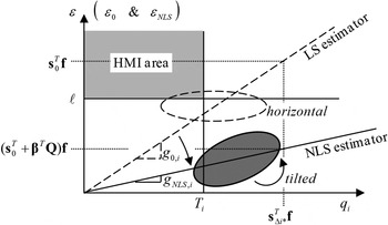
Figure 1. Failure Mode Plot illustrating the new NLS-Estimator-based method versus LS-Estimator-based RAIM.
Let ℓ be the alert limit and  $T_i $ the detection threshold for q i. ℓ is a predefined requirement, and, as explained in Part 1, T i is set to limit the probability of false alarms, for example, following the equation: $T_i = Q^{ - 1} \{ {{C_{REQ} } / {(2nP_{H0} )}}\} $ where C REQ is the continuity risk requirement, and the function Q −1{} is the inverse tail probability of the standard normal distribution. Both ℓ and C REQ are specified for an example aviation application in RCTA Special Committee 159 (2004).
In Figure 1, ℓ and  $T_i$ define the boundaries of the HMI area in the upper left-hand quadrant (shadowed in light grey). One single fault hypothesis $H_i $ is first considered. Under $H_i $, the probability of being in the HMI area is the integrity risk. Lines of constant joint probability density are ellipses because ε and $q_i $ are normally distributed. As the fault magnitude varies, the means of ε and of q i describe a ‘fault mode line’ passing through the origin, with slope g 0,i for the LS estimator, and g NLS,i for the NLS estimator.
For the LS estimator,  $\varepsilon _0 $ and $q _i $ are statistically independent, so that the major axis of the dashed ellipse is either horizontal or vertical. In contrast, using a NLS estimator provides the means to move the dark ellipse away from the HMI area, hence reducing the integrity risk. The influence of the estimator modifier vector ${\bf \beta} $ is threefold.
• The fact that ${\bf \beta} $ impacts the mean of $\varepsilon _{NLS} $ (in Equations (7) and (9)) enables reduction of the failure mode slope from $g_{0,i} $ to $g_{NLS,i} $, which lowers the integrity risk.
• Off-diagonal components of the covariance matrix
${\bf P}_{\eta i} $ also vary with ${\bf \beta} $ so that the dark ellipse's orientation can be modified, and again, integrity risk can be reduced.• However,
${\bf \beta} $ causes the diagonal element of ${\bf P}_{\eta i} $ corresponding to $\varepsilon _{NLS} $ to increase, which means that the dark ellipse is inflated along the ε-axis in Figure 1. This negative impact will be accounted for in the integrity risk evaluation. The increase in variance of $\varepsilon _{NLS} $ also explains that lowering integrity risk comes at the cost of a decrease in accuracy performance.


Figure 1 only considers one fault hypothesis. But, the estimator modifier vector  ${\bf \beta} $ must be determined to minimise the overall integrity risk, considering all hypotheses H i, for $i = 0,\; \ldots,\; n$ as defined in Part 1 of this work, and as expressed again below. To simplify the calculations in the upcoming derivation, a tight integrity risk bound is given by:
 $$\eqalign{P_{HMI} & = \sum\limits_{i = 0}^n {\mathop {\max }\limits_{\,f_i } } \; {P\left( {\vert \varepsilon _{NLS} \vert \gt \ell, \vert q_1 \vert \lt T_1, \; \ldots, \vert q_h \vert \lt {T_i } \;\big \vert f_i} \right) P_{Hi} } \cr & \le \sum\limits_{i = 0}^n {\mathop {\max }\limits_{\,f_i } } \; {P\left( {\vert \varepsilon _{NLS} \vert \gt \ell, \vert q_i \vert \lt T_i \big \vert f_i} \right)P_{Hi} } \equiv {\bar P}_{HMI}} $$
where, as defined in Part 1, P Hi is the prior probability of occurrence of hypothesis H i (i.e., fault on measurement subset i), and f i is the single-Satellite Vehicle (SV) fault magnitude under H i. Determining the worst-case f i is achieved using a line-search process, also implemented in Lee (Reference Lee1995), Milner and Ochieng (Reference Milner and Ochieng2010) and Jiang and Wang (Reference Jiang and Wang2014). The line search can be avoided using the alternative approach given in Section 3.
The integrity risk bound  ${\bar P}_{HMI} $ in Equation (10) remains relatively tight because, under H i it uses the test ‘ $\vert q_i \vert \lt T_i $’, which is specifically designed to detect H i. To avoid changing notations for the fault-free case (i = 0), the following identity is defined: $\{ \vert\varepsilon _{NLS} \vert \gt \ell, \vert q_0 \vert \lt T_0 \} \equiv \{ \vert \varepsilon _{NLS} \vert \gt \ell \} $.
Because the estimate error  $\varepsilon _{NLS} $ is not derived from a LS estimator, $\varepsilon _{NLS} $ and $q _{i} $ in Equation (10) are correlated. In this case, the integrity risk cannot be evaluated as a product of probabilities, but must be treated as a joint probability. Fortunately, numerical methods are available to compute joint probabilities for multi-variate normally distributed random vectors (Drezner and Wesolowsky, Reference Drezner and Wesolowsky1989).
2.3. Multi-Dimensional Optimisation (MDO)
The problem of finding the  $(n - m) \times 1$ vector ${\bf \beta}$ that minimises the overall integrity risk can be mathematically formulated using the bound ${\bar P}_{HMI} $ defined in Equation (10) as: $\mathop {\min} \limits_{\bf \beta} {\bar P}_{HMI} $. An equivalent expression using notations used in Equation (8) is given by:
 $$\mathop {\min }\limits_{\bf \beta } \sum\limits_{i = 0}^n \mathop {\max }\limits_{\,f_i} \left[{\int_{ - \infty }^{ - \ell } {\int_{ - T_i }^{T_i} {\,f_{{\bf \eta }_i } \left( {\varepsilon _{NLS} ,\;{ {q_i} } } \right)\; d \; { {q_i} } \; d\varepsilon _{NLS} } } } + {\int_\ell ^{ + \infty } {\int_{ - T_i }^{T_i } {\,f_{{\bf \eta }_i } \left( {\varepsilon _{NLS} ,\;{ {q_i}} } \right) d\matrix{ {q_i } } d\varepsilon _{NLS} } } }\right]{P_{Hi} } $$
where  $f_{{\bf \eta }_i} \left( {\varepsilon _{NLS},\; {q_i}} \right) = \displaystyle{1 \over {2\pi \; \det ({\bf P}_{\eta i})}} \exp \left( { - \displaystyle{1 \over 2}({\bf \eta}_i - {\bf \mu }_{\eta i} )^T {\bf P}_{\eta i}^{ - 1} ({\bf \eta }_i - {\bf \mu }_{\eta i} )} \right)$
This MDO problem can be solved numerically using a modified Newton method (e.g., see (Luenberger and Ye, Reference Luenberger and Ye2008)). The n scalar search processes to find the worst-case fault magnitude  $f_i^{} $, for i = 1, …, n, are performed at each iteration of the Newton method. Also, the gradient and Hessian of the objective function in Equation (11) can be established numerically using procedures given in Luenberger and Ye (Reference Luenberger and Ye2008). This process is computationally intensive, and is not intended for real time implementation. Computational efficiency will be addressed in Section 3.
The minimisation process outputs an estimator modifier vector  ${\bf \beta} $, which is analysed in comparison with the LS estimator for the six-satellite geometry displayed in Figure 2. In this illustrative example, the two methods are evaluated assuming uncorrelated ranging measurements with a one metre standard deviation, and a prior probability of fault P Hi of 10−4. Example navigation requirements include an integrity risk requirement I REQ of 10−7, a continuity risk requirement C REQ of 8·10−6, and an alert limit ℓ of 15 m.
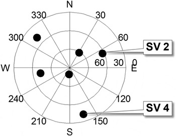
Figure 2. Azimuth-elevation Sky Plot for an example satellite geometry.
Figures 3 and 4 present failure mode plots similar to the one introduced earlier in Figure 1. The same colour code as in Figure 1 is employed: failure mode lines and ellipses of constant joint probability density are represented using solid lines and dark grey areas for the new NLS-estimator-based method versus dashed lines when using the LS estimator. The ellipses are labelled in terms of  $ - \log _{10} f_{{\bf \eta} i} (\varepsilon, \; q_i^{} )$, where $f_{{\bf \eta} i} (\varepsilon, q_i )$ is defined in Equation (11), and ε stands for either $\varepsilon _0 $ or $\varepsilon _{NLS} $. The 10−2 joint probability density level is emphasised for illustration purposes.
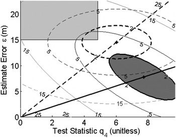
Figure 3. Failure mode plot for the single-SV fault hypothesis on SV4 (worst slope using LS).
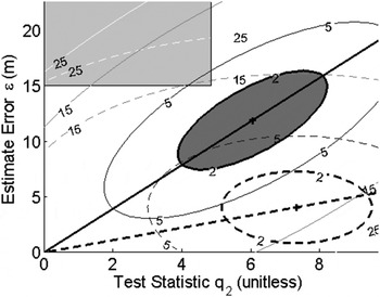
Figure 4. Failure mode plot for the single-SV fault hypothesis on SV2 (worst slope using NLS).
Figure 3 shows joint probability distributions for the hypothesis of a single-satellite fault on SV4 (in this case, the test statistic on the horizontal axis is  $q_4 $). This is the fault mode for which the highest fault slope $g_{0,i} $ was observed using the LS estimator. Because of the large value of $g_{0,i} $, the dashed ellipse for the 10−2 density level overlaps the HMI area. In contrast, using the new method, the black, solid fault mode line has a gentler slope $g_{NLS,i} $, so that the grey-shadowed ellipse avoids penetrating the HMI area.
Figure 4 presents the case of a single-SV fault on SV2, for which the highest fault slope  $g_{NLS,i} $ using the NLS estimator was observed. The fault slope g NLS,i (solid line) is higher than the original slope $g_{0,i} $ using the LS estimator (dashed line). However, the grey-shadowed ellipse's orientation was modified so that the ellipse does not extend over the HMI area.
Figures 3 and 4 show two mechanisms through which the new algorithm using the NLS estimator avoids penetrating the HMI area. The new method reduces the integrity risk under  $H_4 $ in Figure 3, but it does the opposite under $H_2 $ in Figure 4. This is because β is determined in Equation (11) such that the total integrity risk is minimised over all hypotheses. The ellipses corresponding to all six single-SV fault hypotheses are represented in Figure 5, with solid black lines for the LS estimator (labelled DIRE LS for Direct Integrity Risk Evaluation using LS estimator), and with grey shadowed areas for the NLS estimator (labelled DIRE MDO because ${\bf \beta} $ is obtained from a MDO process). Figure 5 shows one ellipse for the DIRE LS overlapping the HMI area, whereas none of the grey-shadowed ellipses for DIRE MDO does.
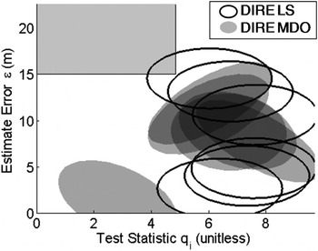
Figure 5. Failure mode plot displaying all single-SV fault hypotheses.
In this example, the integrity risk decreases from 4·7·10−6 for the LS estimator to 3·6·10−8 using the DIRE MDO method. The price to pay for this integrity risk reduction is an increase in the vertical position estimate standard deviation from 1·49 m using DIRE LS to 2·02 m using DIRE MDO (further analysis of the positioning standard deviation is carried out in Section 4 of this paper).
These results show that using a NLS estimator in RAIM can dramatically reduce the integrity risk. However, the MDO process used to determine the optimal  ${\bf \beta} $ vector is extremely time intensive. In Section 3, the DIRE MDO method is further analysed to reduce the computation load.
3. PRACTICAL APPROACH TO NON-LEAST-SQUARES ESTIMATOR DESIGN
This section uses a parity space representation to establish an approximation of the optimal estimator modifier vector β using a One-Dimensional Optimisation (ODO) process instead of the Multi-Dimensional Optimisation (MDO) procedure described in Section 2. Further reduction in computation load is accomplished using an Integrity risk Bound (IB) or using Protection Levels (PL) rather than performing Direct Integrity Risk Evaluation (DIRE).
3.1. One-Dimensional Optimization (ODO)
Under a single-SV fault hypothesis H i, the fault vector is expressed as:  ${\bf f}_i = {\bf A}_i f_i $, where $f_i $ is the fault magnitude, and Ai is defined under Equation (5). Substituting the above expression of ${\bf f}_i $ for ${\bf f}$ into Equation (9), and using the expression of q i in terms of ${\bf p}$ in Equation (5), Equation (9) becomes:
 $${\bf \mu} _{\eta i} = \left[ {\matrix{ {g_{0,i} + \beta \; \rho _{\beta, i}} \cr 1 \cr}} \right]f_{i{^\ast}} \quad {\rm and}\quad {\bf P}_{\eta i} = \left[ {\matrix{ {\sigma _0^2 + \beta ^2} & {\beta \; \rho _{\beta, i}} \cr {\beta \; \rho _{\beta, i}} & 1 \cr}} \right]$$
where
 $$\beta ^2 = {\bf \beta} ^T {\bf \beta}, \quad \rho _{\beta, i} = {\bf u}_\beta ^T {\bf u}_i \quad {\rm with}\quad {\bf u}_\beta = {\bf \beta} \beta ^{ - 1} $$
 $$f_{i{^\ast}} = ({\bf A}_i^T {\bf Q}^T {\bf QA}_i )_{}^{1/2} f_i \quad {\rm and}\quad g_{0,i} = {\bf s}_0^T {\bf A}_i ({\bf A}_i^T {\bf Q}^T {\bf QA}_i )_{}^{ - 1/2} = \sigma _{\Delta i} $$
 In the above equations, β and  ${\bf u}_\beta $ respectively designate the magnitude and unit direction vector of ${\bf \beta} $. Also, it was shown in Joerger et al. (Reference Joerger, Chan and Pervan2014) that $g_{0, \;i} $ can be written as: $g_{0, \;i} = \sigma _{\Delta i} $, where $\sigma _{\Delta i} $ is defined in the paragraph above Equation (3).
The optimal (n − m) × 1 vector  ${\bf \beta} $ obtained using the DIRE MDO method is displayed in parity space in Figure 6(a) for the example six-SV geometry introduced in Figure 2. In this example, the dimension of the parity space is $(n - m) = 2$ because the number of measurements n is six, and the number of states m is four. Single-SV fault lines are represented in grey. In parallel, consider the maximum single-SV fault mode slope $\mathop {\max }\limits_{i = 1, \ldots. ,n} \{ g_{0,i}\} $ for the LS estimator. In Figure 6, the fault line corresponding to the maximum failure mode slope $\mathop {\max }\limits_{i = 1, \ldots. ,n} \{ g_{0,i}\} $ is represented in black.
Let  ${\bf u}_j $ be the unit direction vector in parity space of the fault line corresponding to $\mathop {\max} \limits_{i = 1, \ldots. ,n} \{ g_{0,i} \} $. Figure 6(a) shows that the direction of the optimal ${\bf \beta} $ vector in parity space is very close to that of uj. The same observation is made for many other satellite geometries, including the examples in Figure 6(b) and (c). Conversely, Figure 6(d) shows one of the few examples where the optimal ${\bf \beta} $ direction does not match uj. For this example, the failure mode plot (not represented here) would show that there is a second failure mode whose slope approaches $\mathop {\max} \limits_{i = 1, \ldots. ,n} \{ g_{0,i} \} $. Thus, the optimal ${\bf \beta} $-direction is somewhere between the directions of the two fault lines for these two dominating fault modes. For most other geometries, the maximum fault slope is an outlier-slope, i.e., is much larger than the other n − 1 single-SV slopes. Therefore, in the vast majority of cases, the direction of the optimal ${\bf \beta} $ vector in parity space matches the direction of ${\bf u}_j $.
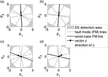
Figure 6. Comparison of DIRE MDO vector  ${\bf \beta} $ versus worst-case fault line directions in parity space.
It follows from the analysis in Figure 6, that a reasonable simplification relative to MDO is to approximate the optimal  ${\bf \beta} $ vector as: β = −β uj, where $j = \arg \mathop {\max }\limits_{i = 1, \ldots. ,n} g_{0,i} $. (The minus sign is included so that only positive values of β need to be considered.) The estimator modifier vector ${\bf \beta} $ can now be determined by finding the value of β, which minimises the integrity risk, i.e., by solving Equation (11) over the scalar parameter β instead of over vector β. This is an ODO process that can be performed using a straightforward line search routine.
It is worth noting that an approximation of the optimal β-direction is sufficient to guarantee that the NLS estimator will perform equally or better than the LS estimator, because the search over β includes the value β = 0, for which LS and NLS estimators are identical. Moreover, the search over β can be limited to ensure that the accuracy requirement is satisfied: accuracy is directly related to the variance  $\sigma _{NLS}^2 $ of $\varepsilon _{NLS} $ (in Equation (12), $\sigma _{NLS}^2 = \sigma _0^2 + \beta _{}^2 $). For example, if the accuracy limit is noted ℓ ACC, then the 95% accuracy criterion is: $2\sigma _{NLS} \lt \ell _{ACC} $, which is equivalent to: $\beta \lt (\ell _{ACC}^2 /4 - \sigma _0^2 )^{1/2} $.
With this choice of  ${\bf u}_\beta $ (as ${\bf u}_\beta = - {\bf u}_j $), an equivalent expression for the NLS estimator is obtained using Equation (5) (as a reminder, Equation (5) is ${\bf s}_{\Delta j ^{\ast}}^T {\bf z} = {\bf u}_j^T {\bf Qz}$):
 $$\eqalign{& {\hat x}_{NLS} \equiv {\bf s}_0^T {\bf z} - \beta {\bf s}_{\Delta j{^\ast}}^T {\bf z},\quad {\rm or \; equivalently},\quad \hat x_{NLS} = {\bf s}_0^T {\bf z} - \beta _{^\ast} {\bf s}_{\Delta j}^T {\bf z}\quad {\rm where}\cr & \quad \beta _{^\ast} = \beta /\sigma _{\Delta j}}$$
 Thus the minimisation problem in Equation (11) can fully be expressed in terms of scalars and vectors already used in SS RAIM: matrix Q does not need to be computed. For example, ρ β,i in Equation (13) becomes  $\rho _{\beta ,i} = - {\bf s}_{\Delta j}^T {\bf s}_{\Delta i} /(\sigma _{\Delta j} \sigma _{\Delta i} )$, and using Equation (14), f i* can be written in terms of: $({\bf A}_i^T {\bf Q}^T {\bf QA}_i )^{1/2} = {{\sigma _{\Delta i}} / {{\bf s}_0^T {\bf A}_i }}$.
The ODO estimator design process can be summarised with the following three steps.
• Find j such that
$j = \arg \mathop {\max} \limits_{i = 1, \ldots ,n} \sigma _{\Delta i} $.• Given that the NLS state estimate is expressed as:
${\hat x}_{NLS} = ({\bf s}_0^T - \beta _{\ast} {\bf s}_{\Delta j}^T ){\bf z}$, find the mean and covariance of ${\bf \eta} _i $, for i = 1,…, n, as a function of $\beta _{\ast} $ using Equations (12) to (15).• Vary
$\beta _{\ast} $ ($\beta _{\ast} \ge 0$) until the minimum integrity risk is found (i.e., solve Equation (11) over β *), or, to speed up the process, until the integrity risk drops below I REQ.


Figure 7 shows that, for the example used in Figures 2 to 6(a), DIRE ODO matches DIRE MDO very closely. The integrity risk only increases from 3·6 × 10−8 to 5·1 × 10−8 for MDO versus ODO, which is still a dramatic reduction as compared to the 4·7 × 10−6 value obtained using DIRE LS. In addition, DIRE ODO is computationally much more efficient than DIRE MDO. Despite this improvement in run time, the DIRE method is still not fit for real time implementations, mainly because the process involves integration in Equation (11) of the bivariate normal density functions of  ${\bf \eta} _i $, for $i = 1, \ldots, n$ (run-time will be quantified in Section 4). In response, an IB is derived.
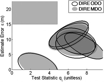
Figure 7. Failure mode plot comparing DIRE MDO versus DIRE ODO.
3.2. Integrity Risk Bounding Method (IB)
In parallel to the minimisation problem over the estimator modifier  ${\bf \beta} $, the DIRE method includes two other time-consuming steps: (a) the integration of the bivariate normal distribution of vector ${\bf \eta} _i = [\matrix{ {\varepsilon _{NLS}} & {q_i} \cr} ]^T $ in Equation (11), and (b) the scalar search over $f_i $ expressed in Equation (10). Both points are addressed using IB, which are looser than using DIRE, but are much faster to evaluate. IB are also more robust than DIRE because they do not require that the correlation between estimate error and test statistic be accurately modelled. And, IB provide a convenient means to deal with nominal measurement error distributions with unknown, bounded, non-zero mean (Blanch et al., Reference Blanch, Walter, Enge, Wallner, Fernandez, Dellago, Ioannides, Hernandez, Belabbas, Spletter and Rippl2013), which DIRE does not.
The IB, once converted into protection levels, take the same form as conventional SS RAIM approaches (Brenner, Reference Brenner1996; Blanch et al., Reference Blanch, Ene, Walter and Enge2007). In this work, the IB are implemented assuming a NLS estimator. The following paragraphs are a step-by-step derivation from Equation (10) to a protection level equation. For analytical purposes in Section 4, the IB-based estimator design process is derived both using MDO and ODO.
First, it is worth remembering that the integration of bivariate normal distributions was needed to evaluate the integrity risk because  $\varepsilon _{NLS} $ and q i are correlated. To avoid dealing with bivariate normal distributions, a bound on the integrity risk in Equation (10) is established using conditional probabilities as follows:
 $$\eqalign{{\bar P}_{HMI} & \le \sum\limits_{i = 0}^n {P\left( {\vert \varepsilon _{NLS} \vert \gt \ell \left. \right \vert \; H_i, \; \vert q_i \vert \lt T_i } \right)P\left( {\vert q_i \vert \lt \left. {T_i } \right \vert H_i } \right)P_{Hi} } \cr & \le \sum\limits_{i = 0}^n {P\left( {\vert \varepsilon _{NLS} \vert \gt \ell \left. \right \vert \; H_i, \; \vert q_i \vert \lt T_i } \right)P_{Hi} }}$$
where, in anticipation of the next steps of the derivation, the condition is expressed in terms H i as in Part 1 (Joerger et al, Reference Joerger, Stevanovic, Langel and Pervan2015), instead of  $f_i$.
It was shown in (Joerger et al., Reference Joerger, Chan and Pervan2014) that the bound  $$P(\vert q_i \vert \lt T_i\vert \; H_i ) = 1$ in the last inequality could be loose. This upper bound is conventionally used in SS RAIM, and is the price to pay to significantly reduce the processing time.
Second, in order to evaluate the above expression independently of fault magnitude (which impacts  $\varepsilon _{NLS} $ and q i), the estimation error for $\hat x_{NLS} $ in Equation (15) is expressed as:
 $$\varepsilon _{NLS} = \left( {{\bf s}_0^T - \beta _\ast {\bf s}_{\Delta j}^T } \right) {\bf z} = {\bf s}_i^T {\bf v} + \left( {{\bf s}_{\Delta i}^T - \beta _\ast {\bf s}_{\Delta j}^T } \right)\left( {{\bf v} + {\bf f}_i } \right)$$
where s0 is written as:  ${\bf s}_0 = {\bf s}_i + {\bf s}_0 - {\bf s}_i,\; {\bf s}_{\Delta i}$ is defined above Equation (3) as: ${\bf s}_{\Delta i} = {\bf s}_0 - {\bf s}_i$
fi is defined above Equation (12),  $\beta _{\ast} $ is defined in Equation (15) and ${\bf s}_i^T {\bf f}_i = {\bf 0}$ under H i.
The term  $({\bf s}_{\Delta i}^T - \beta _{\ast} {\bf s}_{\Delta j}^T )({\bf v} + {\bf f}_i )$ is a function of the fault magnitude. To eliminate this dependency, a new detection test statistic is considered:
 $$\Delta _{NLSi} \equiv \left( {{\bf s}_{\Delta i}^T - \beta _{\ast} {\bf s}_{\Delta j}^T } \right) {\bf z} = \left( {{\bf s}_{\Delta i}^T - \beta _{\ast} {\bf s}_{\Delta j}^T } \right)\left( {{\bf v} + {\bf f}_i^{} } \right)\quad {\rm for}\,\,i = 1, \ldots ,h$$
with variance  $\sigma _{\Delta NLSi}^2 = \sigma _{\Delta i}^2 - 2{\bf s}_{\Delta j}^T {\bf s}_{\Delta i}^{} \beta _{\ast} + \beta _{\ast}^2 \sigma _{\Delta j}^2 $. The associated threshold is given by:
 $$T_{\Delta NLSi} = T_i \sigma _{\Delta NLSi}. $$
 Using  $\Delta _{NLSi} $ instead of q i, substituting Equation (18) into Equation (17) and the result into Equation (16), and using the condition in Equation (16) (which is rewritten as $\vert \Delta _{NLSi}\vert < T_{\Delta NLSi}$), the following integrity risk bound is obtained:
 $$P_{HMI} \le P\left( { \vert \varepsilon _{NLS} \vert \gt \ell \left. \right \vert H_0} \right)P_{H0} + \sum\limits_{i = 1}^n {P\left( { \vert \varepsilon _i \vert + T_{\Delta NLSi} \gt \ell \; \left. \right \vert \; H_i} \right)P_{Hi}} \equiv \overline{\overline P} _{HMI} $$
Equation (20) is then exploited for the integrity risk bounding process using one-dimensional optimisation, also called the ‘IB ODO’ method. The scalar  $\beta _{\ast} $ is found by solving $\mathop {\min} \limits_{\beta _{\ast}} \{ \overline{\overline P} _{HMI} \} $. If required, and as described in the paragraph above Equation (15), the search over $\beta _{\ast} $ can be limited by the accuracy criterion to the values: $0 \le \beta _{\ast} \lt (\ell _{ACC}^2 /4 - \sigma _0^2 )^{1/2} /\sigma _{\Delta j} $.
It is worth noting that Equation (20) can be evaluated for both single-SV and multi-SV faults, since SS RAIM variables and parameters, including  $\varepsilon _i $ and $T_{\Delta NLSi}^{} $ can all be defined assuming subsets of one or more measurements being simultaneously faulted (see multi-SV SS RAIM implementations in Blanch et al. (Reference Blanch, Walter and Enge2012) and Joerger et al. (Reference Joerger, Chan and Pervan2014)).
In addition, for analytical purposes in Section 4, integrity monitoring performance will also be evaluated using IB but without making the assumption in Section 3.1, in a process labelled ‘IB MDO’ (which stands for integrity risk bounding method, using multi-dimensional optimisation). In this case, the direction of  ${\bf \beta }$ is not fixed a priori, and must be determined together with its magnitude. The problem is formulated similar to the above IB ODO, but by replacing $ - \beta _{\ast} {\bf s}_{\Delta j} $ in Equations (17) to (18) with ${\bf \beta } $. The variance $\sigma _{\Delta NLSi}^2 $ can then be expressed as $\sigma _{\Delta NLSi}^2 = \sigma _{\Delta i}^2 + 2\rho _{\beta ,i} \beta \sigma _{\Delta i} + \beta^2 $, and ${\bf \beta }$ is found by solving $\mathop {\min }\limits_{\bf \beta } \{ \overline{\overline P} _{HMI} \} $. In this case, a Newton method is implemented: the gradient vector and Hessian matrix of $\overline{\overline P} _{HMI} $ are expressed analytically in Appendix, following a derivation similar to the one given by Blanch et al. (Reference Blanch, Walter and Enge2012) for a PL-based method.
Given  ${\bf \beta} $, the new detection test statistic $\Delta _{NLSi} $ departs from the solution separation statistic $q_i $ (or equivalently from $\Delta _i = q_i \sigma _{\Delta i} $). In Figure 8, the detection boundaries derived from $\Delta _{NLSi} $ (represented with a thick black contour) and $q_i $ (grey shadowed area) are compared in parity space, for the example satellite geometry presented in Figure 2. (β in Figure 8 was obtained using the IB MDO method.) In LS SS RAIM, projections of the parity vector p onto the fault lines (represented with thin black lines intersecting at the origin), i.e., along ${\bf u}_i $, define the test statistics q i, as expressed in Equation (5). Projections of p onto lines in the direction of ${\bf u}_i^{} + {\bf \beta} $ (thin grey lines) define the new statistics $\Delta _{NLSi} $.
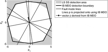
Figure 8. Detection region for LS SS versus the Integrity risk Bounding (IB) method.
Figure 8 shows only a small change between the LS SS detection boundary and that of the NLS SS obtained using IB MDO. When considering realistic system parameters and requirements, this modification is not expected to cause a dramatic increase or decrease in integrity risk. Practical implementations of multiple SS RAIM implementations in Blanch et al. (Reference Blanch, Ene, Walter and Enge2007) and of chi-squared residual based RAIM in Joerger et al. (Reference Joerger, Chan and Pervan2014) show little sensitivity of  $P_{HMI}^{} $ to such changes in the detector as compared to the impact of the bounding process in Equations (16) and (20).
Finally, the same MDO and ODO processes can be applied to PL equations. The protection level  $p_L $ can be solved iteratively using the following equation (Blanch et al., Reference Blanch, Ene, Walter and Enge2007; Blanch et al., Reference Blanch, Walter and Enge2012).
 $$P\left( { \vert \varepsilon _{NLS} \vert \gt p_L \;\left. \right \vert\; H_0} \right)P_{H0} + \sum\limits_{i = 0}^n {P\left( { \vert \varepsilon _i \vert + T_{NLS,\Delta i} \gt p_L \; \left. \right \vert \; H_i} \right)P_{Hi}} = I_{REQ} - P_{NM} $$
Aside from the additional step in Equation (21) (which makes PL determination more computationally intensive than IB), the PL approach is almost identical to the IB method. The PL MDO process is described in detail in (Blanch et al., Reference Blanch, Walter and Enge2012). It requires significantly more computation resources than when applying the proposed ODO method to PL equations. This comparison is quantified in Section 4.
4. AVAILABILITY AND COMPUTATION TIME EVALUATION
This section aims to analyse the integrity risk reduction and rise in processing time generated when implementing a NLS estimator as compared to using a LS estimator in SS RAIM. The algorithms derived in Sections 2 and 3 are evaluated in an example Advanced RAIM (ARAIM) application for vertical guidance of aircraft using dual-frequency GPS and Galileo. The simulation parameters, which include ARAIM measurement error models, and LPV-200 navigation requirements (to support localiser precision vertical aircraft approach operations down to 200 feet above the ground), are listed in Table 1 and described in detail in (EU-US Cooperation on Satellite Navigation, 2012). In this analysis, two major differences with respect to the ARAIM error models are that constellation-wide faults are not accounted for, and that fault-free measurement biases are assumed to be zero. These biases introduce application-specific complications whose treatment is not relevant to this paper. Also to simplify the analysis, accuracy requirements were not included in the availability assessment (but can easily be incorporated in the  ${\bf \beta} $-determination process as described in Section 3).
Table 1. Simulation Parameters.
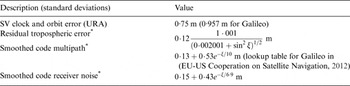
* : ξ is the satellite elevation angle in degrees.
Example navigation requirements include an integrity risk requirement  $I_{REQ} $ of 10−7, and a continuity risk requirement $C_{REQ} $ of 10−6. The prior probability of satellite fault $P_{Hi} $ is assumed to be 10−5. The alert limit ℓ is reduced from 35 m in ARAIM (EU-US Cooperation on Satellite Navigation, 2012) to 10 m in this performance evaluation. A ‘24-1’ GPS satellite constellation and a ‘27-1’ Galileo constellation are assumed, which are nominal constellations with one spacecraft removed to account for outages; these example constellations are also described in EU-US Cooperation on Satellite Navigation (2012). Moreover, this analysis focuses on the vertical position coordinate, for which the aircraft approach navigation requirements are often the most difficult to fulfil.
Figure 9 displays availability maps for a 10° × 10° latitude-longitude grid of locations, for GPS/Galileo satellite geometries simulated at regular five minute intervals over a 24 hour period. Availability is computed at each location as the fraction of time where the  $P_{HMI} $ bound (derived using either DIRE or IB) meets the integrity risk requirement $I_{REQ} $. In the figures, availability is colour-coded: white colour corresponds to a value of 100%, black represents 80%. Constant availability contours are also displayed. The worldwide availability metric given in the figure caption is the average over all grid points of the availability weighted by the cosine of the latitude, because grid point locations near the equator represent larger areas than near the poles.
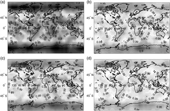
Figure 9. Availability Maps for: (a) Integrity Risk Bounding Method (IB) Using Least Squares Estimator: Worldwide Weighted Average Availability (WWAA) is 92·6%; (b) IB Using Multi-Dimensional Optimisation (MDO): WWAA is 97·4%; (c) IB Using One-Dimensional Optimisation (ODO): WWAA is 96·7%; (d) Direct Integrity Risk Evaluation (DIRE) Using ODO: WWAA is 98·1%.
Figure 9(a) presents availability for the IB method using a LS estimator, i.e., using a conventional SS RAIM method. Then Figure 9(b) shows the availability that can potentially be achieved using a NLS estimator derived from a MDO method. In practice, if computational resources are too limited to solve the MDO problem, then the ODO process can be implemented, and the corresponding availability map is shown in Figure 9(c). Average availability using ODO is 96·7% versus 97·4% using MDO, but it is still much higher than the 92·6% value obtained using a LS estimator in Figure 9(a).
In addition, Figure 9(d) displays the availability provided by direct integrity risk evaluation (DIRE) using ODO to determine the NLS estimator. The DIRE MDO method would probably have generated slightly higher availability, but the computation time to generate an availability map would have exceeded several months. Thus, the 98·1% worldwide average availability value for DIRE ODO is our closest approximation of the best availability that can be reached using a NLS estimator and a LS SS detector.
Average availability numbers are listed in Table 2 for the DIRE, IB and PL methods (PL given in parentheses), using a LS estimator, or using the MDO or ODO processes to determine a NLS estimator. The third column of Table 2 shows the inflation of the vertical position estimate standard deviation caused by the use of a NLS estimator rather than a LS estimator. This factor  $\sigma _{NLS} /\sigma _0^{} $ can cause the accuracy performance to diminish, but for all algorithms, the inflation factor averaged over all locations and satellite geometries remains lower than 1·04. Also, as mentioned in Section 3, the accuracy requirement can be built into the NLS estimator design algorithm to ensure that the accuracy criterion remains satisfied when it is initially met for the LS estimator.
Table 2. Simulation Results.
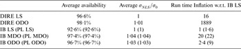
The fourth column in Table 2 gives the inflation in computation time for each algorithm as compared to the IB LS computation time. The reference IB LS run time is 0·8 ms per geometry. These numbers were generated on a computer equipped with a 3·40 GHz Intel(R) Core(TM) i7-2600 processor and 8 GB RAM. Computation times can be analysed in parallel with worldwide average availability results in the second column of Table 2. The IB MDO achieves 97·4% availability, but the run time inflation factor is 20. The IB ODO method accomplishes an effective compromise between run time and availability performance: availability using IB ODO increases from 92·6% to 96·7% with respect to IB LS, but the run time is only about twice that of IB LS.
Availability results using the PL equations are identical to the IB method since the two methods make the same assumptions. However, the run times are longer using PL because an extra iterative process must be implemented to solve for  $p_L^{} $ in Equation (21).
Finally, the DIRE ODO method provides 98·1% average availability. This number is higher than for any other algorithm, but the computation time is almost 2000 times larger than for a more conventional IB LS method that would probably be impractical for most real time applications. In years to come, improvements in embedded processing and computing technology may enable real-time implementation of DIRE ODO, which would then provide a significant increase in availability.
5. CONCLUSION
This paper is Part 2 of a two-part research effort, which describes new methods to minimise the integrity risk by design of the RAIM detector and estimator, for applications in future multi-constellation GNSS-based navigation.
Part 1 shows illustrative examples suggesting that, using a Least-Squares (LS) estimator and for realistic navigation requirements, the optimal detection region approaches the SS detection boundary. Therefore, the new RAIM methods are devised using test statistics derived from SS RAIM.
This paper (i.e., Part 2) investigates the potential of reducing the integrity risk using a Non-Least-Squares (NLS) estimator. The first method, labelled DIRE (which stands for Direct Integrity Risk Evaluation), aims at minimising integrity risk regardless of computation load, and provides a measure of the best achievable integrity performance. This method is computationally expensive. As an alternative, a second method labelled IB ODO (for integrity risk bounding, using One-Dimensional Optimisation) is developed using parity space representations and failure mode plots. Despite conservative assumptions in the integrity risk bounding process, IB ODO still significantly lowers integrity risk as compared to using a LS estimator, but also considerably reduces processing load with respect to other NLS estimator design methods.
Performance analyses are carried out for an example aircraft approach application using multi-constellation Advanced RAIM. For a given set of navigation system parameters, the worldwide average availability provided by IB ODO is slightly lower than the best achievable performance (evaluated using DIRE), but is substantially higher than using a LS estimator. In addition, IB ODO does not significantly degrade the accuracy performance as compared to a LS estimator. Finally, the IB ODO processing time is only about twice that of a conventional LS SS RAIM algorithm, and is five to ten times shorter than for the other NLS estimator design methods, which may enable real time implementation in applications where computation resources are limited.
ACKNOWLEDGMENTS
The authors would like to thank the Federal Aviation Administration for sponsoring this work.
APPENDIX. GRADIENT AND HESSIAN DERIVATION FOR THE OPTIMAL ESTIMATOR USING THE ‘IB MDO’ METHOD
This appendix presents a derivation of the gradient vector and Hessian matrix for IB MDO method, i.e., to solve the minimisation problem ‘ $\min \{ \overline{\overline P} _{HMI} \} $’ over the (n − m) × 1 vector ${\bf \beta} $. The derivation is similar to the one given in Blanch et al. (Reference Blanch, Walter and Enge2012), but differences exist because the objective function in Blanch et al. (Reference Blanch, Walter and Enge2012) is different from $\overline{\overline P}_{HMI}$, which is defined in equation (20). $\overline{\overline P} _{HMI} $ can be further bounded as:
 $$\eqalign{&{\overline{\overline P}} _{HMI} \le \bar P_{HMI{^\ast}} \left( {\bf \beta} \right)\quad {\rm where}\cr & \quad \bar P_{HMI{^\ast}} \left( {\bf \beta} \right) = \underbrace {2Q\left( {\ell \sigma _{NLS}^{ - 1} \left( {\bf \beta} \right)} \right)}_{\bar P_{HMI,0}} + \sum\limits_{i = 1}^n {\underbrace {Q\left( {\left( {\ell - T_{\Delta NLSi} ({\bf \beta} )} \right)\sigma _i^{ - 1}} \right)}_{\bar P_{HMI,i}} P_{Hi}}}$$
The main reason for using Equation (A1) rather than Equation (20) is to lighten notations. It is worth noting that the terms  ${\bar P}_{HMI,i} $ only account for the side of the Gaussian distribution where most of the probability density is concentrated. The other side of the distribution corresponds to a much smaller probability (amounting to $Q( - (\ell + T_{\Delta NLSi} )/\sigma _i )$), which is conservatively accounted for in a subtle way, by multiplying $\bar P_{HMI,0}$ by 1 instead of $P_{H0} $.
The following notations are used in the derivation. First, Equation (19) is rewritten as:  $T_{\Delta NLSi} ({\bf \beta} ) = T_i \sigma _{\Delta NLSi} ({\bf \beta} )$. Then, the standard deviation of the NLS estimate error is expressed as:
 $$\sigma _{NLS}^2 = \sigma _0^2 + \beta ^2 = \Vert {{\bf s}_0^T + {\bf \beta }^T {\bf Q}} \Vert^2 = \Vert {{\bf r}_0 } \Vert^2 \rm \;where \;{\bf r}_0 = {\bf Q\,s}_0+{\bf \beta}$$
and where  $\Vert {\bf r} \Vert$ is the 2-norm of vector ${\bf r}$: $\left\vert {\bf r} \right\vert ^2 = {\bf r}^T {\bf r}$. The (n − m) × 1 gradient vector and (n − m) × (n − m) Hessian matrix of ${\overline P}_{{HMI}^{\ast}}$ in Equation (A1) are respectively given by:
 $$\nabla {\bar P_{HMI^{\ast}}} = \displaystyle{\partial \over {\partial {\bf \beta }}}{\bar P_{HMI^{\ast}}} = \nabla {\bar P_{HMI,0}} + \sum\limits_{i = 1}^n {\nabla {{\bar P}_{HMI,i}}{P_{Hi}}} $$
 $$H\left\{ {{\bar P}_{HMI^{\ast}} } \right\} = \nabla \left\{ {\nabla \bar P_{HMI^{\ast}} } \right\} = H\left\{ {{\bar P}_{HMI,0} } \right\} + \sum\limits_{i = 1}^n {H\left\{ {{\bar P}_{HMI,i} } \right\}} P_{Hi} $$
The rest of this appendix gives a derivation for each term in Equations (A3) and (A4).
Fault-Free Terms:
Substituting Equation (A2) into (A1), the (n − m) × 1 gradient vector  $\nabla {\bar P}_{HMI,0} $ can be expressed as: $\nabla {\bar P}_{HMI,0} = 2\nabla Q(\ell \Vert{\bf r}_0 \Vert^{ - 1} )$. Using the chain rule, and the fact that ∂Q(y)/∂y = −φ(y), where φ(y) is the probability density function of a standard normal distribution, $\nabla {\bar P}_{HMI,0} $ can be written as:
 $$\nabla {\bar P}_{HMI, 0} = 2\ell \Vert {\bf r}_0 \Vert ^{ - 3} \phi \left( {\ell \Vert{\bf r}_0 \Vert ^{ - 1}} \right) {\bf r}_0 = 2\ell \sigma _{NLS}^{ - 3} \phi \left( {\ell \sigma _{NLS}^{ - 1}} \right) {\bf r}_0 $$
where we used Equation (A2) and the following result:  $$\nabla \Vert {{\bf r}_0 } \Vert = {{{\bf r}_0} / {\Vert {{\bf r}_0 } \Vert}}$.
Then, the (n − m) × (n − m) Hessian matrix  $H\left\{ {\bar P_{HMI,0}} \right\}$ is the gradient of the product in Equation (A5), and is expressed as:
 $$H\left\{ {\bar P_{HMI,0}} \right\} = \nabla \left\{ {2\ell \phi \left( {\ell \Vert {\bf r}_0 \Vert ^{ - 1}} \right)} \right\}{\bf r}_0 \Vert {\bf r}_0 \Vert ^{ - 3} + 2\ell \phi \left( {\ell \Vert {\bf r}_0 \Vert ^{ - 1}} \right) \nabla \left\{ {{\bf r}_0 \Vert {\bf r}_0 \Vert ^{ - 3}} \right\}$$
Using ∂φ(y)/∂y = −yφ(y) and using the chain rule, the following equation is established:
 $$\nabla \left\{ {2\ell \phi \left( {\ell \Vert {\bf r}_0 \Vert ^{ - 1}} \right)} \right\} = \ell ^2 \Vert {\bf r}_0 \Vert ^{ - 1} 2\ell \Vert {\bf r}_0 \Vert ^{ - 3} \phi \left( {\ell \Vert {\bf r}_0 \Vert ^{ - 1}} \right) {\bf r}_0 = \ell ^2 \Vert {\bf r}_0 \Vert ^{ - 1} \nabla \bar P_{HMI,0} $$
In parallel, the following result is derived:
 $$\nabla \left\{ {{\bf r}_0 \Vert {\bf r}_0 \Vert ^{ - 3}} \right\} = \Vert {\bf r}_0 \Vert ^{ - 3} \left( {{\bf I}_{n - m} - 3{\bf r}_0 {\bf r}_0^T \Vert {\bf r}_0 \Vert ^{ - 2}} \right)$$
Finally, substituting Equations (A7) and (A8) into Equation (A6), and substituting Equation (A2) into the resulting equation, yields the following expression:
 $$H\left\{ {\bar P_{HMI,0}} \right\} = \ell ^2 \sigma _{NLS}^{ - 4} {\bf r}_0 \nabla P_{HMI,0}^T + 2\ell \sigma _{NLS}^{ - 3} \phi \left( {\ell \sigma _{NLS}^{ - 1}} \right)\left( {{\bf I}_{n - m} - 3{\bf r}_0 {\bf r}_0^T \sigma _{NLS}^{ - 2}} \right)$$
Terms Corresponding to Fault Hypotheses:
First, similar to Equation (A2), the variance of the NLS solution separation for subset i is given by:  $\sigma _{\Delta NLSi}^2 = \Vert{\bf r}_i \Vert^2 $, where ${\bf r}_i = {\bf Qs}_{\Delta i} + {\bf \beta} $. Substituting $\sigma _{\Delta NLSi}^2 $ into the above expression of $T_{\Delta NLSi} ({\bf \beta} )$, and the result into (A1), and following the same steps as in Equations (A3) to (A5), the (n − m) × 1 gradient vector $\nabla \bar P_{HMI,i} $ can be expressed as:
 $$\nabla \bar P_{HMI,i} = \nabla Q\left( {(\ell - T_i \Vert {\bf r}_i \Vert )\sigma _i^{ - 1}} \right) = \phi \left( {(\ell - T_{\Delta NLSi} )\sigma _i^{ - 1}} \right) T_{\Delta NLSi} \sigma _i^{ - 1} \sigma _{\Delta NLSi}^{ - 2} {\bf r}_i $$
 Then, following the same steps as in Equations (A6) to (A9),  $H\left\{ {\bar P_{HMI,i}} \right\}$ is given by:
 $$H\left\{ {\bar P_{HMI,i}} \right\} = \displaystyle{{T_{\Delta NLSi}} \over {\sigma _i^2 \sigma _{\Delta NLSi}^2}} \left[ {\left( {\ell - \displaystyle{{T_{\Delta NLSi}} \over {\sigma _{\Delta NLSi}^2}}} \right){\bf r}_i \nabla P_{HMI,i}^T + \phi \left( {\displaystyle{{\ell - T_{\Delta NLSi}} \over {\sigma _i}}} \right) \left( {{\bf I}_{n - m} - \displaystyle{{{\bf r}_i {\bf r}_i^T} \over {\sigma _{\Delta NLSi}^2}}} \right)} \right]$$
Finally,  $\nabla \bar P_{HMI^{\ast}} $ and $H\left\{ {\bar P_{HMI^{\ast}}} \right\}$ are respectively obtained by substituting Equations (A5) and (A10) into Equation (A3), and by substituting Equations (A9) and (A11) into Equation (A4).


