


1. Introduction
Interactions between fluid flows and phase boundaries are key to understanding a wide range of phenomena in both the natural (Meakin & Jamtveit Reference Meakin and Jamtveit2010) and engineered environments (Kurz & Fisher Reference Kurz and Fisher1984). Such interactions occur at scales ranging from the microscopic (Wettlaufer & Worster Reference Wettlaufer and Worster2006) to the macroscopic (Maslowski et al. Reference Maslowski, Clement Kinney, Higgins and Roberts2012; Hewitt Reference Hewitt2020), and have a controlling effect on the evolution of many systems, including the Earth's interior (Deguen, Alboussiere & Cardin Reference Deguen, Alboussiere and Cardin2013) and its polar regions (McPhee Reference McPhee2008; Ramudu et al. Reference Ramudu, Hirsh, Olson and Gnanadesikan2016), and the icy moons (Walker & Schmidt Reference Walker and Schmidt2015; Soderlund et al. Reference Soderlund2020), to name a few.
Fluid flows over phase boundaries are due principally to buoyancy forces generated because of thermal and/or compositional gradients during phase change (Davis, Müller & Dietsche Reference Davis, Müller and Dietsche1984; Dietsche & Müller Reference Dietsche and Müller1985; Huppert Reference Huppert1990; Wettlaufer, Worster & Huppert Reference Wettlaufer, Worster and Huppert1997; Worster Reference Worster1997; Wykes et al. Reference Wykes, Huang, Hajjar and Ristroph2018) and/or mean shear flows (Delves Reference Delves1968, Reference Delves1971; Gilpin, Hirata & Cheng Reference Gilpin, Hirata and Cheng1980; Coriell et al. Reference Coriell, McFadden, Boisvert and Sekerka1984; Forth & Wheeler Reference Forth and Wheeler1989; Feltham & Worster Reference Feltham and Worster1999; Neufeld & Wettlaufer Reference Neufeld and Wettlaufer2008a,Reference Neufeld and Wettlauferb; Bushuk et al. Reference Bushuk, Holland, Stanton, Stern and Gray2019), which in some cases were introduced to control morphological instabilities. However, in certain instances, when there is a free surface associated with the liquid layer, its dynamics can also play an important role in the evolution of the solid phase (Meakin & Jamtveit Reference Meakin and Jamtveit2010). Here, we focus on the effects of a phase boundary on the thermal and thermocapillary instabilities associated with such a liquid layer. Specifically, we study the interplay between these two modes of instability in a film of water, which has a temperature of maximum density, overlying a layer of pure ice. Thermal instability in this case leads to penetrative convection (Veronis Reference Veronis1963; Toppaladoddi & Wettlaufer Reference Toppaladoddi and Wettlaufer2018).
Thermal instability in the presence of a phase boundary was first studied systematically by Davis et al. (Reference Davis, Müller and Dietsche1984) and Dietsche & Müller (Reference Dietsche and Müller1985) using weakly nonlinear stability analysis and experiments. The working fluid used in their experiments was cyclohexane, which has a linear equation of state and hence does not exhibit anomalous behaviour. A key finding of their study is that the critical Rayleigh number and wavenumber for the onset of instability first decrease monotonically with the thickness of the solid phase (scaled by the thickness of the liquid phase) and then asymptote to constant values for large values of the solid-phase thickness (Davis et al. Reference Davis, Müller and Dietsche1984). Furthermore, the convection patterns (rolls, hexagons, or a combination of both), as observed on the underside of the solid phase, were also found to depend on the initial dimensionless thickness of the solid layer. More recent studies have explored these interactions in the laminar (Favier, Purseed & Duchemin Reference Favier, Purseed and Duchemin2019; Purseed et al. Reference Purseed, Favier, Duchemin and Hester2020; Toppaladoddi Reference Toppaladoddi2021) and turbulent (Esfahani et al. Reference Esfahani, Hirata, Berti and Calzavarini2018; Ravichandran & Wettlaufer Reference Ravichandran and Wettlaufer2021) regimes.
The effects of a free liquid surface on phase change have been studied to understand the formation of icicles (Makkonen Reference Makkonen1988; Szilder & Lozowski Reference Szilder and Lozowski1994; Short, Baygents & Goldstein Reference Short, Baygents and Goldstein2006) and stalactites (Short et al. Reference Short, Baygents, Beck, Stone, Toomey III and Goldstein2005a; Short, Baygents & Goldstein Reference Short, Baygents and Goldstein2005b), and the rippled patterns on them (Ogawa & Furukawa Reference Ogawa and Furukawa2002; Ueno Reference Ueno2007; Camporeale, Vesipa & Ridolfi Reference Camporeale, Vesipa and Ridolfi2017). Liquid film over an icicle aids in the transport of latent heat generated during phase change to the ambient air, whereas over a stalactite it transports CO $_2$ produced by the chemical reaction between water and CaCO $_3$. In both these cases, the shear flow is driven by gravity, and the transport across the liquid film is due only to diffusion. Similar rippled patterns have been observed on a layer of ice subjected to a shear- and buoyancy-driven turbulent flow over it in the presence of a free surface (Gilpin et al. Reference Gilpin, Hirata and Cheng1980; Toppaladoddi & Wettlaufer Reference Toppaladoddi and Wettlaufer2019). Furthermore, in the presence of a free surface, gradients in surface tension make the liquid layer susceptible to stationary and oscillatory thermocapillary instabilities (Takashima Reference Takashima1981a,Reference Takashimab).
Previous studies have also explored the effects of shear flows on phase-boundary evolution, with the experiments of Gilpin et al. (Reference Gilpin, Hirata and Cheng1980) being one of the first systematic studies. In their set-up, a turbulent shear flow of water was maintained over a layer of ice in a closed-loop water tunnel with a free surface. The temperature boundary conditions were such that the temperature far from the ice–water interface was above the melting point. A perturbation was initially introduced at the ice–water interface by melting a semi-cylindrical groove in the ice layer. Gilpin et al. (Reference Gilpin, Hirata and Cheng1980) observed that under certain conditions, this initial perturbation grew, leading to a ‘rippled’ surface, which impacted considerably the heat flux to the ice–water interface. Although these effects were attributed solely to the mean shear flow (Gilpin et al. Reference Gilpin, Hirata and Cheng1980), Toppaladoddi & Wettlaufer (Reference Toppaladoddi and Wettlaufer2019), using Monin–Obukhov theory, showed that there were substantial buoyancy effects due to the anomalous behaviour of water. However, the potential effects of a free surface on the system's dynamics remain unclear. Camporeale & Ridolfi (Reference Camporeale and Ridolfi2012) studied a free-surface induced morphological instability of an inclined ice–water interface using a linear stability analysis, ignoring buoyancy effects in the liquid. For thin films, buoyancy effects are indeed negligible (Kalliadasis et al. Reference Kalliadasis, Ruyer-Quil, Scheid and Velarde2011), and thermal effects influence only via interfacial effects, as was done in the linear stability analysis of Jiang, Cheng & Peng (Reference Jiang, Cheng and Peng2020) for a vertical falling film on an ice sheet. When the assumption of thin films is relaxed, buoyancy effects will have non-negligible effects. Bushuk et al. (Reference Bushuk, Holland, Stanton, Stern and Gray2019) studied experimentally the formation of ice scallops on an inclined open-channel flow down an ice slab. In their experiments, the air temperature was maintained at 0 $\,^{\circ }$C to ensure that melting happens predominantly due to heat transfer between water and ice. Suppose that the air temperature is marginally higher than the melting temperature. In that case, buoyancy effects in ice–water melting problems where a water layer overrides the ice can be significant due to the nonlinear equation of state. A 10 cm water layer overlying an ice layer with a 0.2 K temperature difference across the depth would have a Rayleigh number of $ O (10^6)$, indicating the behaviour to be well into the regime of turbulent convection (Taylor & Feltham Reference Taylor and Feltham2004).
The combined effects of the anomalous behaviour of water, the free surface and a melting bottom boundary are also potentially important in the evolution of melt ponds over sea ice, especially during the early stages of growth. Melt ponds form due to the melting of the snow layer overlying sea ice during the transition from winter to summer. This transition impacts considerably the effective albedo and thus the radiation budget in the Arctic. Surface melting of the sea ice in the Arctic region accounts for approximately 50 % of the total melted volume, with lateral and bottom melting accounting for the rest (Maykut & Perovich Reference Maykut and Perovich1987). Hence there have been recent efforts to take the convective flow inside melt ponds into account, with Taylor & Feltham (Reference Taylor and Feltham2004) providing a heat transfer model for pond–ice systems. Subsequently, Skyllingstad & Paulson (Reference Skyllingstad and Paulson2007) performed large-eddy simulations to study turbulent convection in various melt pond geometries. Recently, Kim et al. (Reference Kim, Moon, Wells, Wilkinson, Langton, Hwang, Granskog and Rees Jones2018) made in situ measurements of vertical temperature profiles inside a freshwater pond and a saline pond to understand the role of salinity on net heat fluxes. They also performed direct numerical simulations of the freshwater and saline water layers exposed to air on the top and bottom boundary maintained at the melting point, highlighting the asymmetric mode of convection due to the nonlinear equation of state. However, in these simulations, the bottom boundary was assumed to be rigid, ignoring phase change.
These studies on the flow dynamics in melt ponds are in the turbulent regime. However, to our knowledge, the problem of onset of convection in a liquid layer confined between a free surface and a phase boundary has not been explored. Hirata, Goyeau & Gobin (Reference Hirata, Goyeau and Gobin2012) studied the linear stability of under-ice melt ponds, focusing on the onset of convective instabilities owing to both salt and temperature stratifications. They studied a three-layer system comprising a melt pond, an ice matrix and an under-ice melt pond, and found that increasing ice layer thickness enhanced the system's instability. However, they considered both the air–water and water–ice boundaries to be rigid. In the absence of strong temperature gradients within ice, thermal convection modifies dramatically the geometry of the phase boundary (Ravichandran & Wettlaufer Reference Ravichandran and Wettlaufer2021), and the solid phase in turn has considerable effect on the stability of the liquid layer (Davis et al. Reference Davis, Müller and Dietsche1984; Toppaladoddi & Wettlaufer Reference Toppaladoddi and Wettlaufer2019; Toppaladoddi Reference Toppaladoddi2021). Hence it is necessary to include the Stefan condition in the study of fluid flows over phase boundaries.
Some of the key questions that emerge from the studies of Gilpin et al. (Reference Gilpin, Hirata and Cheng1980) and Hirata et al. (Reference Hirata, Goyeau and Gobin2012) are the following. (i) What are the effects of a free surface on the evolution of an ice–water system? (ii) How does the system evolve in the presence of both stably and unstably stratified layers of liquid? (iii) How does the onset of penetrative convection depend on the thickness of the ice phase? The last question would be an extension to the studies of Davis et al. (Reference Davis, Müller and Dietsche1984) and Dietsche & Müller (Reference Dietsche and Müller1985) for a nonlinear equation of state. In the current study, we seek to understand these effects systematically by considering the linear stability of a layer of water confined between a layer of ice at the bottom and air at the top. The temperature boundary conditions are such that only convective motions can develop above the critical values of Rayleigh and Marangoni numbers. The problem set-up considered here is an idealised version of the melt pond geometry. We do not include an internal heat source and salinity effects, with the latter being more relevant to melt ponds over first-year ice (Kim et al. Reference Kim, Moon, Wells, Wilkinson, Langton, Hwang, Granskog and Rees Jones2018), and focus solely on buoyancy effects due to variations in the temperature field.
The paper is organised as follows. The problem formulation and the equations of motion, along with the boundary conditions, are discussed in § 2. The details of the linear stability analysis and the results obtained are discussed in § 3. We then present the conclusions from our study in § 4.
2. Problem formulation
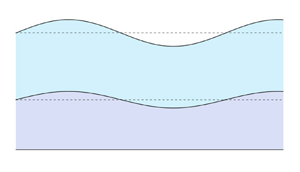
We consider a layer of water confined between a layer of ice at the bottom and a layer of air at the top, as shown in figure 1, in two dimensions. The initial thicknesses of the water and ice layers are  $h$ and $d$, respectively. There are two moving boundaries in the system: the air–water and ice–water interfaces. In the base state, these interfaces are flat. When small perturbations are introduced, the instantaneous locations of the ice–water and air–water interfaces are given by $\eta _1 (x,t)$ and $h + \eta _2 (x,t)$, respectively. The layer of air, the ice–water interface and the bottom plate are maintained at temperatures $T_h$, $T_c$ and $T_i$, respectively, and are such that $T_h>T_c>T_i$. For simplicity, water and ice are assumed to have the same density ( $\rho _0$) and thermal diffusivity ( $\kappa$). The equation of state for water is nonlinear, and is well approximated by (Veronis Reference Veronis1963)
 \begin{equation} \rho(T_l) = \rho_0 [1 - \alpha (T_l - T_m)^2 ], \end{equation}
where  $\rho _0$ is the reference density, $T_l$ is the temperature of water, $T_m$ is the temperature of maximum density, and $\alpha$ is the coefficient of thermal expansion. This density profile has a maximum ( $=\rho _0$) at $T_l = T_m$. If $T_h > T_m$, then there is a layer of stably stratified fluid overlying a layer of unstably stratified fluid (see figure 2). It is also evident from figure 2 that the depths of the stable and unstable layers are dependent on the values of $T_h$ and $T_m$. With increasing values of $T_h$, the depth of the stably stratified layer increases. Table 1 lists the values of the relevant physical parameters for an ice–water system. In the following, we discuss the equations of motion for the different parts of the domain.

Figure 1. Schematic of a film of water over an ice sheet. The deformations in the ice–water and air–water interfaces are exaggerated for better illustration.

Figure 2. Base state (a) temperature and (b) density profiles of the liquid layer drawn with  $T_h = 8\,^{\circ }C$, ${T_c = 0\,^{\circ}}C$ and $T_m = 4\,^{\circ }C$, and the corresponding density profile obtained using (2.1). Plot (b) also shows the regions of stable and unstable density stratification.
Table 1. Estimates of physical parameters for an ice–water–air system at 277 K.

2.1. Water
The dynamics in the water layer is described by the continuity, momentum balance and heat balance equations, which are obtained after making the Boussinesq approximation and are given by (Chandrasekhar Reference Chandrasekhar2013)
 $$\begin{gather} \boldsymbol{\nabla}\boldsymbol{\cdot} \boldsymbol{u} = 0, \end{gather}$$
 $$\begin{gather}\frac{\partial \boldsymbol{u}}{\partial t} + \boldsymbol{u} \boldsymbol{\cdot} \boldsymbol{\nabla} \boldsymbol{u} ={-} \frac{1}{\rho_0}\,\boldsymbol{\nabla} P + \nu\,\nabla^2 \boldsymbol{u} + [1 - \alpha (T_l - T_m)^2] \boldsymbol{g} \end{gather}$$
and
 \begin{equation} \frac{\partial T_l}{\partial t} + \boldsymbol{u} \boldsymbol{\cdot}\boldsymbol{\nabla} T_l = \kappa\,\nabla^2 T_l. \end{equation}
Here,  $\boldsymbol {u} = (u,v)$ is the velocity filed, $\nu$ is the kinematic viscosity, $P$ is the pressure field, and $\boldsymbol {g}$ is the acceleration due to gravity.
2.2. Ice
In the ice layer, the temperature field  $T_s$ is governed by the diffusion equation:
 \begin{equation} \frac{\partial T_s}{\partial t} = \kappa\,\nabla^2 T_s. \end{equation}
2.3. Ice–water interface
The dynamics of the ice–water interface is governed by the Stefan condition, which – for small amplitudes of interfacial deformation – is given by
 \begin{equation} \rho_0 L_s\,\frac{\partial \eta_1}{\partial t} = \boldsymbol{n} \boldsymbol{\cdot} [\boldsymbol{q}_l - \boldsymbol{q}_s]_{y = \eta_1}. \end{equation}
Here,  $L_s$ is the latent heat of fusion, $\boldsymbol {q}_s$ and $\boldsymbol {q}_l$ are the conductive heat fluxes into the ice from the interface and from the water layer towards the interface, respectively, and $\boldsymbol {n}$ is the outward unit normal at the interface, given by
 \begin{equation} \boldsymbol{n} = \frac{1}{\sqrt{1 + (\partial \eta_1/\partial x)^2}} \left(- \frac{\partial \eta_1}{\partial x},1\right). \end{equation}
2.4. Boundary conditions
We impose the following boundary conditions at the different interfaces.
(i) The temperature boundary condition at the bottom plate ( $y = -d$) is given by
(2.8)\begin{equation} T_s = T_i. \end{equation}
$y = -d$) is given by
(2.8)\begin{equation} T_s = T_i. \end{equation}(ii) The velocity and temperature boundary conditions at the ice–water interface (
$y = \eta _1(x,t)$) are
(2.9)$$\begin{gather} \boldsymbol{u} \boldsymbol{\cdot} \boldsymbol{n} = \boldsymbol{u} \boldsymbol{\cdot} \boldsymbol{t} = 0, \end{gather}$$(2.10)Here,$$\begin{gather}T_s = T_l = T_c. \end{gather}$$$\boldsymbol {t}$ is the unit tangent at the interface.(iii) The balances of normal and tangential stresses at the air–water interface (
$y=h + \eta _2(x,t)$) are
(2.11)\begin{align} P &= \frac{2 \mu}{ \left[ 1 + \left( \dfrac{\partial \eta_2}{\partial x} \right) ^2 \right]} \left[ \frac{\partial u}{\partial x} \left( \frac{\partial \eta_2}{\partial x} \right) ^2 - \left( \frac{\partial v}{\partial x} + \frac{\partial u}{\partial y} \right) \frac{\partial \eta_2}{\partial x} + \frac{\partial v}{\partial y} \right] \nonumber\\ &\quad - \frac{\sigma\,\dfrac{\partial ^2 \eta_2}{\partial x ^2}}{\left[ 1 + \left( \dfrac{\partial \eta_2}{\partial x} \right) ^2\right] ^{3/2}}, \end{align}(2.12)Here,\begin{align} & \mu \left[ 4\,\frac{\partial u}{\partial x}\,\frac{\partial \eta_2}{\partial x} - \left( 1 - \left( \frac{\partial \eta_2}{\partial x} \right) ^2 \right) \left( \frac{\partial u}{\partial y} + \frac{\partial v}{\partial x} \right) \right] \nonumber\\ &\quad = \gamma \left( \frac{\partial\eta_2}{\partial x}\,\frac{\partial T_l}{\partial y} + \frac{\partial T_l}{\partial x} \right) \sqrt{1 + \left( \frac{\partial \eta_2}{\partial x} \right) ^2}. \end{align}$\sigma = \sigma _0 - \gamma (T_l - T_h)$ is the surface tension, and $\gamma = - ({\rm d} \sigma / {\rm d} T)|_{T_a}$.(iv) At the air–water interface (
$y=h_0 + \eta _2(x,t)$), we consider Newton's law of cooling:
(2.13)Here,\begin{equation} \mathcal{K} \boldsymbol{n} \boldsymbol{\cdot}\boldsymbol{\nabla} T_l ={-} \chi (T_l - T_h). \end{equation}$\mathcal {K}$ is the thermal conductivity of water, and $\chi$ is the heat transfer coefficient. A discussion of the above imperfect heat transfer between the overlying air and the underlying phase can be found in Hitchen & Wells (Reference Hitchen and Wells2016). Although Hitchen & Wells (Reference Hitchen and Wells2016) derived the boundary condition in the context of sea ice growth, it remains valid as a model for the interface of a melt pond (Kim et al. Reference Kim, Moon, Wells, Wilkinson, Langton, Hwang, Granskog and Rees Jones2018).(v) The kinematic boundary condition at the air–water interface (
$y=h_0 + \eta _2(x,t)$) is
(2.14)\begin{equation} \frac{\partial \eta_2}{\partial t} + u\,\frac{\partial \eta_2}{\partial x} = v. \end{equation}


The above system of equations is made dimensionless using the height  $h$ as the length scale, $u_0 = \kappa / h$ as the velocity scale, $P_0 = \rho \nu \kappa / h^2$ as the pressure scale, and ${\rm \Delta} T = T_h - T_c$ as the temperature scale. With the Rayleigh number as $Ra = g h^3 \alpha \, {\rm \Delta} T^2 / (\nu \kappa )$, the capillary number as $Ca = \rho \nu \kappa / (\sigma _0 h)$, the Marangoni number as $Ma = \gamma \,{\rm \Delta} T\,h / (\rho \nu \kappa )$, the Prandtl number as $Pr = \nu / \kappa$, the Stefan number as $\mathcal {S} = L_s / (c_p\,{\rm \Delta} T)$, the Biot number as $Bi = \chi h / K$, $\lambda = {\rm \Delta} T / (T_m - T_c)$ and $\zeta = \alpha (\lambda (T_m-T_c))^2$, the dimensionless equations are given by
 $$\begin{gather} \boldsymbol{\nabla} \boldsymbol{\cdot} \boldsymbol{u} = 0, \end{gather}$$
 $$\begin{gather}\frac{\partial \boldsymbol{u}}{\partial t} + \boldsymbol{u} \boldsymbol{\cdot}\boldsymbol{\nabla} \boldsymbol{u} = Pr\,[-\boldsymbol{\nabla} P + \nabla^2 \boldsymbol{u} - Ra\,(\zeta^{{-}1} - \theta_l^2) \boldsymbol{y}], \end{gather}$$
 $$\begin{gather}\frac{\partial \theta_l}{\partial t} + \boldsymbol{u} \boldsymbol{\cdot} \boldsymbol{\nabla} \theta_l = \nabla^2 \theta_l, \end{gather}$$
 $$\begin{gather}\frac{\partial \theta_s}{\partial t} = \nabla^2 \theta_s , \end{gather}$$
and the dimensionless boundary conditions are:
(i) at
$y = - d/h$,
(2.19)\begin{equation} \theta_s = \theta_i; \end{equation}(ii) at
$y = \eta _1$,
(2.20)$$\begin{gather} u = v = 0, \end{gather}$$(2.21)$$\begin{gather}\theta_s = \theta_l = \theta_c, \end{gather}$$(2.22)$$\begin{gather}\frac{\partial \eta_1}{\partial t} ={-} \frac{1}{\mathcal{S} \sqrt{1 + \left( \dfrac{\partial \eta_2}{\partial x} \right)^2}} \left\lbrace \frac{\partial}{\partial y} (\theta_l - \theta_s) - \frac{\partial \eta_1}{\partial x}\,\frac{\partial}{\partial x} (\theta_l - \theta_s) \right\rbrace; \end{gather}$$(iii) at
$y = 1 + \eta _2$,
(2.23)\begin{align} P &= \frac{2}{ \left[ 1 + \left( \dfrac{\partial \eta_2}{\partial x} \right) ^2 \right]} \left[ \frac{\partial u}{\partial x} \left( \frac{\partial \eta_2}{\partial x} \right) ^2 - \left( \frac{\partial v}{\partial x} + \frac{\partial u}{\partial y} \right) \frac{\partial \eta_2}{\partial x} + \frac{\partial v}{\partial y} \right] \nonumber\\ &\quad -\frac{ \left[ Ca^{{-}1} + Ma \left( \theta_l - \theta_h \right) \right] \dfrac{\partial ^2 \eta_2}{\partial x ^2}}{\left[ 1 + \left( \dfrac{\partial \eta_2}{\partial x} \right) ^2 \right] ^{3/2}}, \end{align}(2.24)\begin{align} & 4\,\frac{\partial u}{\partial x}\,\frac{\partial \eta_2}{\partial x} - \left( 1 - \left( \frac{\partial \eta_2}{\partial x} \right) ^2 \right) \left( \frac{\partial u}{\partial y} + \frac{\partial v}{\partial x} \right) \nonumber\\ &\quad ={-}Ma\left( \frac{\partial \eta_2}{\partial x}\,\frac{\partial \theta_l}{\partial y} + \frac{\partial \theta_l}{\partial x} \right) \sqrt{1 + \left( \frac{\partial \eta_2}{\partial x} \right) ^2}, \end{align}(2.25)$$\begin{align} &\frac{1}{\sqrt{1 + \left( \dfrac{\partial \eta_2}{\partial x} \right) ^2}} \left\lbrace \frac{\partial \theta_l}{\partial y} - \frac{\partial \eta_2}{\partial x}\, \frac{\partial \theta_l}{\partial x} \right\rbrace ={-} Bi\,(\theta_l - \theta_h), \end{align}$$(2.26)\begin{gather}\frac{\partial \eta_2}{\partial t} + u\,\frac{\partial \eta_2}{\partial x} = v . \end{gather}


Here,  $\theta _l = (T_l - T_m)/{\rm \Delta} T$, $\theta _c = (T_c - T_m)/{\rm \Delta} T$, $\theta _s = (T_s - T_m)/{\rm \Delta} T$ and $\theta _i = (T_i - T_m)/ {\rm \Delta} T$.
The parameter  $\lambda$, as defined by Veronis (Reference Veronis1963), is the ratio between the total depth of the liquid layer and the depth of the unstably stratified layer of the liquid, and is equivalent to the definition used here in the $Bi\rightarrow \infty$ limit. For water, $T_c=0\,^{\circ }$C and $T_m=4\,^{\circ }$C, thus $T_h=4\lambda \,^{\circ }$C. Additionally, we also have the Galilei number, defined as ${Ga} = Ra / \zeta = g h^3 / (\nu \kappa )$ (Velarde, Nepomnyashchy & Hennenberg Reference Velarde, Nepomnyashchy and Hennenberg2001; Lyubimov et al. Reference Lyubimov, Lyubimova, Lobov and Alexander2018). However, since ${Ga}$ cannot be varied independently, we choose not to include it explicitly in our equations. Figure 3 shows the values of the mentioned non-dimensional numbers as functions of the film height.

Figure 3. Non-dimensional numbers plotted for a range of film height  $h$ with ${\rm \Delta} T = 8\,^{\circ }\mathrm {C}$ using the physical parameters listed in table 1.
3. Linear stability analysis
In the base state, there are no fluid motions, and the air–water and ice–water interfaces are planar. The base-state temperature fields in the ice and water layers are obtained by solving the steady-state diffusion equation, and the solutions are given by
 $$\begin{gather} \theta_s^{b} = \theta_c + \frac{\theta_c - \theta_i}{d/h}\,y, \end{gather}$$
 $$\begin{gather}\theta_l^{b} = \theta_c + \frac{Bi}{1+Bi}\,y, \end{gather}$$
where the superscript  $b$ denotes base state. In order for the ice–water interface to remain planar and fixed in the base state, we require that the heat fluxes at the interface balance. This leads to
 \begin{equation} \frac{\theta_c - \theta_i}{d/h} = \frac{Bi}{1+Bi}. \end{equation}
We now introduce normal-mode perturbations in the system with wavenumber  $k$ and wave speed $c$. As a result of this, each physical parameter in the system (say $X$) is given by $X(x,y,t) = X^b(x) + \hat {X}(y) \exp ({{\rm i} k (x - c t)})$, with $X^b$ denoting the base-state value, and $\hat {X}$ denoting the infinitesimally small amplitude of the disturbance ( $|\hat {X}| \ll |X^b|$). Linearising (2.15)–(2.18) about the base state, we get
 $$\begin{gather} \big\{ Pr
\big(\mathcal{D}^2 - k^2\big)^2 + {\rm i}kc
\big(\mathcal{D}^2 - k^2\big) \big\} \hat{v} -
\big\{2 k^2\,Ra\,Pr\,\theta^b_l \big\}
\hat{\theta}_l = 0, \end{gather}$$
$$\begin{gather} \big\{ Pr
\big(\mathcal{D}^2 - k^2\big)^2 + {\rm i}kc
\big(\mathcal{D}^2 - k^2\big) \big\} \hat{v} -
\big\{2 k^2\,Ra\,Pr\,\theta^b_l \big\}
\hat{\theta}_l = 0, \end{gather}$$ $$\begin{gather}\big\{
\mathcal{D}^2 - k^2 + {\rm i} k c \big\}
\hat{\theta}_l - \left\lbrace \frac{{\rm d}
\theta^b_l}{{\rm d}y} \right\rbrace \hat{v} = 0,
\end{gather}$$
$$\begin{gather}\big\{
\mathcal{D}^2 - k^2 + {\rm i} k c \big\}
\hat{\theta}_l - \left\lbrace \frac{{\rm d}
\theta^b_l}{{\rm d}y} \right\rbrace \hat{v} = 0,
\end{gather}$$ $$\begin{gather}\big\{
\mathcal{D}^2 - k^2 \big\} \hat{\theta}_s ={-} {\rm
i} k c \hat{\theta}_s,
\end{gather}$$
$$\begin{gather}\big\{
\mathcal{D}^2 - k^2 \big\} \hat{\theta}_s ={-} {\rm
i} k c \hat{\theta}_s,
\end{gather}$$
with boundary conditions at  $y = - d/h$
 \begin{equation} \hat{\theta}_{s} = 0, \end{equation}
at  $y = 0$
 $$\begin{gather} \mathcal{D} \hat{v} = 0, \end{gather}$$
 $$\begin{gather}\hat{v} = 0, \end{gather}$$
 $$\begin{gather}\frac{{\rm d} \theta^b_s}{{\rm d}y}\,\hat{\eta}_{1} + \hat{\theta}_{s} = 0, \end{gather}$$
 $$\begin{gather}\frac{{\rm d} \theta^b_l}{{\rm d}y}\,\hat{\eta}_{1} + \hat{\theta}_{l} = 0, \end{gather}$$
 $$\begin{gather}\mathcal{D} \hat{\theta}_{l} - \mathcal{D} \hat{\theta}_{s} = {\rm i} k c \mathcal{S} \hat{\eta}_1, \end{gather}$$
and at  $y = 1$
 \begin{gather} \big(\mathcal{D}^2 + k^2 \big) \hat{v} = k^2\,Ma \left(\frac{{\rm d} \theta_l^b}{{\rm d}y}\,\eta_2 + \hat{\theta}_l \right), \end{gather}
 \begin{gather} \big\{{\rm i} k c
\mathcal{D} + Pr \big(\mathcal{D}^2 - 3 k^2\big)
\mathcal{D} \big\} \hat{v} \nonumber\\
\quad - Pr\,k^2 \big\{ Ra \big( \zeta^{{-}1} -
(\theta_l^b)^2 \big) + k^2 \big[ Ca^{{-}1} +
Ma\,(\theta_l^b - \theta_h) \big] \big\}
\hat{\eta}_2 = 0,
\end{gather}
\begin{gather} \big\{{\rm i} k c
\mathcal{D} + Pr \big(\mathcal{D}^2 - 3 k^2\big)
\mathcal{D} \big\} \hat{v} \nonumber\\
\quad - Pr\,k^2 \big\{ Ra \big( \zeta^{{-}1} -
(\theta_l^b)^2 \big) + k^2 \big[ Ca^{{-}1} +
Ma\,(\theta_l^b - \theta_h) \big] \big\}
\hat{\eta}_2 = 0,
\end{gather} $$\begin{gather} {\rm i} k c \hat{\eta}_2 + \hat{v} = 0, \end{gather}$$
 $$\begin{gather}\left( \mathcal{D} + Bi \right) \hat{\theta}_l + Bi\,\frac{{\rm d} \theta^b_l}{{\rm d}y}\, \hat{\eta}_2 = 0. \end{gather}$$
Here,  $\mathcal {D}$ denotes the derivative of the perturbation amplitudes with respect to $y$. The above system of linear equations is similar to the corresponding system obtained for a flow between two parallel plates with a stress-free surface, first derived by Veronis (Reference Veronis1963) without the ice layer. The full system of linear equations (3.4)–(3.16) does not admit an analytical solution. However, as the perturbation temperature field in the ice layer is decoupled from the momentum and temperature perturbation fields in the fluid layer, the analytical solution to (3.6), subject to boundary conditions (3.7) and (3.10), is found to be
 $$\begin{gather} \hat{\theta}_s = a_1 \exp{\big(\sqrt{k(k-{\rm i}c)}\,y\big)} + a_2 \exp{\big(-\sqrt{k(k-{\rm i}c)}\,y\big)}, \end{gather}$$
 $$\begin{gather}a_1 ={-} \frac{Bi}{1+Bi}\,\hat{\eta}_1\,\frac{\exp{\left(2\sqrt{k(k-i c)} d/h\right)}}{\exp{\left(2\sqrt{k(k-i c)}\,d/h\right)}-1}, \end{gather}$$
 $$\begin{gather}a_2 = \frac{Bi}{1+Bi} \hat{\eta}_1 \frac{1}{\exp{\left(2\sqrt{k(k-i c)} d/h\right)}-1}. \end{gather}$$
3.1. Results
We now study the coupling between thermocapillary and thermal instabilities, and the impact of the phase boundary on them, by solving the linearised equations (3.4)–(3.6), along with the boundary conditions (3.7)–(3.16).
3.1.1. Thermocapillary instability
We first wish to understand the effects of convective motions on the thermocapillary instability. To this end, we follow Takashima (Reference Takashima1981a) and study the thermocapillary instability in the limit of small wavenumbers ( $k \ll 1$). By expanding the perturbative quantities in (3.4)–(3.16) in powers of $k$, and solving the equations to $ O (k)$, we obtain the complex wave speed as
 \begin{align} c &= c _0 + k c _1 + {O}(k^2) \nonumber\\ &\approx \frac{1}{\eta_{20}} \int _0 ^1 \hat{u}_0\,{{\rm d}y} + {\rm i} k\, \frac{1}{\eta_{20}} \int _0 ^1 \left( \hat{u}_1 - \frac{\eta_{21}}{\eta_{20}}\, \hat{u}_0 \right) {{\rm d}y} \nonumber\\ &\approx {\rm i} k \left\lbrace \left( \frac{Bi}{1+Bi} \right)^2 \frac{Ra\,(60 + Bi\,(34+27 d/h))}{180(1 + Bi + Bi\,d/h)} + \frac{Bi}{1+Bi}\,\frac{Ra\,\theta_c (40 + Bi\,(29 + 25 d/h))}{60 (1 + Bi + Bi\,d/h)} \right. \nonumber\\ &\quad \left.\vphantom{\left( \frac{Bi}{1+Bi} \right)^2} +\frac{Ra\,\theta_c^2}{3} - \frac{Ga}{3} + \frac{Bi}{(1 + Bi + Bi\,d/h) (1+Bi)}\,\frac{Ma}{2} \right\rbrace. \end{align}
We should note that solutions to the linearised system (3.4)–(3.16) appear only at even powers of  $k$. This becomes apparent if we replace $k c$ with $\omega$, which results in $k$ appearing solely at even powers (implying $c = k c_1 + k^3 c_3 + O (k^5)$) and is due to the absence of a background flow. However, in the presence of a background flow, $c_0 \neq 0$, as in the case of falling films (Yih Reference Yih1963; Dhas & Roy Reference Dhas and Roy2022). For brevity, we have not included the expression for the $ O (k^3)$ correction to the wave speed here (see figure 5 for comparisons against the wave speed obtained numerically). The critical Marangoni number $Ma_c$ is obtained subsequently by setting $c = 0$ in the above equation, giving
 \begin{align} Ma_c &\approx \frac{(1 + Bi + Bi\,d/h) (1+Bi)}{Bi} \left( \frac{2\,Ga}{3} - \frac{2\,Ra\, \theta_c^2}{3} \right) \nonumber\\ &\quad - \frac{Bi\,Ra\,(60 + Bi\,(34+27d/h))}{90 (1+Bi)} - \frac{Ra\,\theta_c (40 + Bi\,(29+25 d/h))}{30}. \end{align}
If we ignore buoyancy and the phase boundary (by setting  $d/h = 0$), impose an adiabatic boundary condition at the air–water surface in the base state, and set $\theta _c = -1$ (which corresponds to the case where $T_m = T_h$), then the critical Marangoni number becomes
 \begin{equation} Ma_{c} = \tfrac{2}{3}\,Ga\,(1 + Bi). \end{equation}
 The above expression is consistent with the result obtained by Takashima (Reference Takashima1981a), thereby demonstrating that our general expression for  $Ma_c$ reduces to this special case. An important implication of result (3.21) is that for $k \ll 1$, $Ma_c$ is independent of the equation of state of the fluid, and is the same for both linear and nonlinear equations of state. This is also evident from (3.4), where the buoyancy term is $ O (k^2)$. We will use this result to discern the effects of penetrative convection on $Ma_c$. We note that we are interested in the marginal states of the stationary thermocapillary instability, wherein both the real and imaginary parts of the wave speed $c$ would be zero. This implies that the small deformations of both the phase boundary and the free surface do not affect the condition for marginal stability as a consequence of the linearisation (see (3.12) and (3.15)).
The equations corresponding to the nonlinear equation of state (3.4)–(3.6), do not admit analytical solutions, but the corresponding equations with a linear equation of state do. Therefore, we first study the system corresponding to the linear equation of state. Note that since we are looking at a system that is hot on top and cold at the bottom, onset of thermal instability is not possible when using a linear equation of state. (Details on the calculations corresponding to the linear equation of state can be found in Appendix A.) We assign the values of the parameters as  $Pr = 11.6$, $\lambda = 2$, $\mathcal {S} = 10$, $Ca = 10^{-6}$ and $Bi = 10$ for all of our subsequent calculations, unless specified otherwise. We also choose the value of $Ra$ as $6000$ to study the thermocapillary instability such that it lies below the critical threshold corresponding to the thermal instability mode for $Ma = 0$ (see § 3.1.2).
In figure 4, we show the neutral stability curves for  $d/h = 0$ (implying the absence of an ice layer), $d/h = 1$ and $d/h = 10$ calculated using the linear equation of state (red curves). It is seen that for a fixed value of $d/h$, the critical Marangoni number decreases with increasing $k$. The criticality threshold decreases until we reach $k = O (1)$. This is again consistent with the results of Takashima (Reference Takashima1981a). The insets in figure 4 show $Ma_c$ as a function of $d/h$ for different fixed values of $k$. For $k \ll 1$, $Ma_c$ increases monotonically with increasing $d/h$. However, for $k = O (1)$ and $k \gg 1$, $Ma_c$ is independent of $d/h$. Hence the effects of phase boundary on the thermocapillary instability for $k = O (1)$ and $k \gg 1$ are qualitatively similar to its effects on Rayleigh–Bénard convection (Davis et al. Reference Davis, Müller and Dietsche1984).

Figure 4. Neutral stability curves drawn in the  $Ma_c$– $k$ plane for $d/h=0$ (solid lines), $d/h=1$ (dashed lines) and $d/h=10$ (dotted lines) with a linear equation of state (red lines) and a nonlinear equation of state (blue lines). The insets depict neutral curves in the $Ma_c$– $d/h$ plane for wavenumbers $k = 10^{-4}$, $2$ and $10$, and ${Ra = 6000}$. The region above the curves is the zone of instability.
Having explored the thermocapillary instability in the absence of penetrative convection, we now study the effects of a nonlinear equation of state by solving (3.4)–(3.5) numerically using the Chebyshev spectral collocation method (Trefethen Reference Trefethen2000). (Further details of the numerical method used are provided in Appendix B.) To validate our numerical code, we reproduce the results of Veronis (Reference Veronis1963) for penetrative convection with the top and bottom boundaries being rigid. The results from this validation are shown in table 2, and are in good agreement. Further, we also compare the wave speed obtained numerically with the long-wave analytical calculation. We obtain excellent agreement in the long-wave limit ( $k \ll 1$) between the analytical and numerical calculations, as shown in figure 5.
Table 2. Comparisons for validation of the stability code with the results by Veronis (Reference Veronis1963) for the rigid boundary case.


Figure 5. The imaginary part of the wave speed ( ${\rm Im}{(c)}$) associated with the thermocapillary instability mode obtained numerically (blue line), from the $ O (k^3)$ long-wave calculation (red solid line) and from the $ O (k)$ long-wave expression in (3.20) (red dashed line). Here, $Ra = 6000$, $Ma = 2 \times 10^8$, $\lambda = 2$, $\mathcal {S} = 10$ and $Bi = 10$.
The marginal stability curves for the case of the nonlinear equation of state (in blue) are shown in figure 4. Comparing the  $Ma_c$ values for the linear and the nonlinear equations of state, we see that there is negligible difference between them for $k < O (1)$ (compare the blue and red lines in figure 4, and the inset for $k = 10^{-4}$). The same can be said for $k \gg 1$ (see the inset for $k = 10$ in figure 4). However, for $k = O (1)$, the values of $Ma_c$ in the presence of penetrative convection are significantly lower than those in the absence of convective motions (see the inset for $k = 2$ in figure 4).
The reason for this difference in behaviour can be seen by studying the eigenfunctions of the temperature disturbance, which are shown in figure 6. We see from these images that for  $k = 10^{-4}$ and $k = 10$, there is no discernible difference between the temperature fields in the presence and absence of penetrative convection. In both cases, the temperature perturbations are mostly confined near the air–water interface. However, for $k = O (1)$, here represented with $k = 2$, we see that the Bénard cells penetrate significantly deeper in the presence of penetrative convection. These findings corroborate what we observed previously with the neutral stability curves in figure 4. It is clear from these results that the coupling between penetrative convection and the thermocapillary instability is established through the disturbance wavenumber. For $k \ll 1$, the effects of buoyancy are not felt; and for $k \gg 1$, the disturbances are confined to a region close to the air–water interface. However, only for $k = O (1)$ do the disturbances penetrate into the unstably stratified region. When ${\rm \Delta} T = 8$, the upper half of the fluid layer is stably stratified and the lower half is unstably stratified. Hence disturbances with $k = O (1)$ are of wavelengths comparable to the thickness of the liquid layer and therefore get stretched when they encounter the unstably stratified region.

Figure 6. Perturbed temperature field with the streamfunction plotted for  $d/h = 0.1$ and $Ra=6000$. The values chosen for $Ma$ are greater than the corresponding $Ma_c$. (a) Linear equation of state, $k = 10^{-4}$, $Ma = 10^{9}$. (b) Nonlinear equation of state, $k = 10^{-4}$, $Ma = 10^{9}$. (c) Linear equation of state, $k = 2$, $Ma = 2000$. (d) Nonlinear equation of state, $k = 2$, $Ma = 2000$. (e) Linear equation of state, $k = 10$, $Ma = 2000$. ( f) Nonlinear equation of state, $k = 10$, $Ma = 2000$.
The results shown in figure 4 were obtained for  $Ra < Ra_c$ in a corresponding system devoid of thermal effects (see § 3.1.2 for details on the thermal instability mode). We next probe the thermocapillary instability for $Ra = 20\,000$, such that both the thermocapillary and thermal instabilities can coexist. The results for such a case are shown in the black curves of figure 7. We find that this higher value of $Ra$ is stabilising for $k \ll 1$, whereas it is destabilising for $k = O (1)$. This destabilisation is due to the emergence of the thermal mode of instability. Yet another aspect is the influence of the depth of penetrative convection dictated by the parameter $\lambda = 2$. Decreasing the value of $\lambda$ increases the depth of the unstable layer, thereby potentially lowering the critical Rayleigh number for the thermal mode of instability. Therefore, as expected, we observe similar trends for the cases $\lambda = 1.5$ and $0.5$ as with the case $Ra = 20\,000$ – stabilising for small values of the wavenumber, and destabilising for $ O (1)$ values of the wavenumber. For $\lambda = 0.5$ ( $T_h = 2$), no penetrative convection exists since the water layer is unstably stratified along its entire depth. The lack of any critical Marangoni number in the region of $ O (1)$ wavenumbers in figure 7 is due to the thermal mode of instability taking over to destabilise the system. We note that for $\lambda = 1.5$ and $0.5$, the critical Rayleigh number corresponding to the thermal instability mode is lower than $6000$. Further details on the thermal instability mode are provided in § 3.1.2.

Figure 7. Neutral stability curves drawn in the  $Ma_c$– $k$ plane for $d/h=1$, $\lambda = 2$ (dashed lines), $\lambda = 1.5$ (solid lines) and $\lambda = 0.5$ (dotted lines), with $Ra = 6000$ (blue) and $Ra = 20\,000$ (black), with a nonlinear equation of state. The insets depict neutral curves in the $Ma_c$– $d/h$ plane for wavenumbers $k = 10^{-4}$ and $10$. The region above the curves is the zone of instability.
In addition to the effects of the nonlinear equation of state, we also explore the impact of the Stefan number ( $\mathcal {S}$) on the thermocapillary instability. Figure 8 shows the neutral stability curves plotted for $\mathcal {S} = 1$ and 10. From (3.12), it is clear that variations in $\mathcal {S}$ will not have any impact on the stability threshold associated with the stationary thermocapillary instability mode being studied here. This is because $\mathcal {S}$ drops out of (3.12), since the wave speed is zero at the marginal states of the stationary instability mode. However, ${\rm Re}{(c)} \neq 0$ for the oscillatory instability mode. Therefore, we probe the influence of Stefan number by computing the neutral curves for the oscillatory instability (see the inset in figure 8). We find that the region of instability expands with an increase in Stefan number from $\mathcal {S} = 1$ to $\mathcal {S} = 10$. We also find the instability region expands significantly with an increase in thickness of the ice layer. Despite this, it is important to note that the oscillatory instability is not particularly relevant to ice–water systems since we find that it is triggered only at Marangoni numbers of $ O (10^8)$ or higher. Such Marangoni numbers are associated with water layers that are a few metres in thickness (see figure 3). Regnier, Dauby & Lebon (Reference Regnier, Dauby and Lebon2000), in their analysis, also note that the oscillatory thermocapillary instability is not possible under realistic conditions on Earth under the Boussinesq approximation. Therefore, we restrict the study of the oscillatory thermocapillary instability only to highlight the influence of the Stefan number. As expected, we find no perceivable change in the critical Marangoni numbers corresponding to the stationary thermocapillary instability.

Figure 8. Neutral stability curves drawn in the  $Ma_c$– $k$ plane for $d/h=1$ (dashed lines) and $d/h=10$ (dotted lines), with $\mathcal {S} = 10$ (blue) and $\mathcal {S} = 1$ (red), with a nonlinear equation of state. The bottom left inset shows the oscillatory thermocapillary instability, for which the region enclosed by the curves is unstable. The other insets depict neutral curves in the $Ma_c$– $d/h$ plane for wavenumbers $k = 2$ and $10$, and $Ra = 6000$.
3.1.2. Thermal instability
The Marangoni stresses are not the only source of instability in this system. As noted previously, due to the anomalous behaviour of water, we have a base state in which a part of the liquid layer is unstably stratified. We now study this thermal mode of instability in the absence of Marangoni stresses ( $Ma = 0$). In figures 9(a) and 9(b), the dependence of the critical Rayleigh number $Ra_c$ and critical wavenumber $k_c$ on $d/h$ is shown for $Bi = 10$ and $100$. For a fixed value of $Bi$, we find that both $Ra_c$ and $k_c$ first decrease with increasing $d/h$, and then asymptote to constant values ( $Ra_c \approx 10\,248$, $k_c \approx 2.85$ for $Bi = 10$, and $Ra_c \approx 13\,840$, $k_c \approx 3.3$ for $Bi = 100$). Thus we find that the presence of the phase boundary has a destabilising effect. This is again qualitatively consistent with the results of Davis et al. (Reference Davis, Müller and Dietsche1984) for Rayleigh–Bénard convection over a phase boundary. The reason for this destabilising effect is that in the limit $d/h \rightarrow 0$, the ice layer becomes a perfect conductor, and the classical case is recovered. However, in the opposite limit, $d/h \rightarrow \infty$, the ice layer becomes a poor conductor and more susceptible to deformations, and hence less stable (Davis et al. Reference Davis, Müller and Dietsche1984).

Figure 9. Neutral stability curves for Biot numbers  $Bi = 10$ (solid lines) and $Bi = 100$ (dashed lines), with $Ma = 0$. The region above the curves is the zone of instability.
Between the two values of  $Bi$ studied, we find that the higher value yields more stability (see figure 9a). The reason for this is the following. When the free surface is insulated ( $Bi = 0$), temperature perturbations are easier to set up. However, when the free surface can convect heat, as would be the case for large $Bi$, any temperature perturbations introduced would decay (Nield Reference Nield1964). This is evident from the thermal boundary condition prescribed at the free surface (see (3.16)). Thus larger values of the temperature gradient are required to destabilise the system for increasing values of $Bi$ (Nield Reference Nield1964).
We next study the influence of the depth of penetrative convection on the system's stability. Figures 10(a) and 10(b) show the critical Rayleigh number and wavenumber, respectively, for three values of  $\lambda$, namely 0.5, 1.5 and 2. We find that in the cases $\lambda = 0.5$ and $1.5$, the stability thresholds drop significantly in comparison to the case $\lambda = 2$, throughout the range of $d/h$ explored. As discussed previously, lowering the value of $\lambda$ would increase the depth of the unstable layer, thereby producing this destabilising effect. These observations are also consistent with the results obtained by Veronis (Reference Veronis1963). Furthermore, we also studied the influence of the Stefan number on the thermal instability mode, and found that this does not affect the critical Rayleigh number. This is qualitatively consistent with the results of Toppaladoddi & Wettlaufer (Reference Toppaladoddi and Wettlaufer2019).

Figure 10. Neutral stability curves for  $\lambda = 0.5$ (red), $\lambda = 1.5$ (black) and $\lambda = 2$ (blue), with $Bi = 10$ and $Ma = 0$. The region above the curves is the zone of instability.
To understand the influence of Marangoni stresses on the thermal instability, we now solve the equations with  $Ma > 0$. In figures 11(a) and 11(b), the dependence of $Ra_c$ on $Ma$ and $k$ is shown, respectively. We see that an increase in $Ma$ decreases the stability threshold. Hence, as noted by Nield (Reference Nield1964), the Marangoni stresses and the destabilising buoyancy forces act together to destabilise the system. Beyond a critical Marangoni number, $Ra_c$ drops to zero. This is attributed to the thermocapillary instability becoming dominant. This is evident from the neutral curves shown figure 11(a). The switch from thermal to thermocapillary instability is seen to occur at $Ma \approx 550$, $450$ and $430$ for $d/h = 0$, $1$ and $10$, respectively. The value $Ma = 500$ was chosen to highlight that $Ra_c = 0$ for $d/h = 1$ and $10$, but $Ra_c$ is non-zero for $d/h = 0$. Therefore, the neutral curves corresponding to the thermocapillary and thermal modes (marked as ‘TC’ and ‘T’, respectively, in figure 11b) can be seen to be well separated for $d/h = 0$, but merged together for $d/h = 1$ and $10$. We also find that the stability threshold decreases further in the presence of an ice layer.

Figure 11. Neutral stability curve in (a) the  $Ra$–
$Ra$– $Ma$ plane and (b) the $Ra$–
$Ra$– $k$ plane, for $d/h=0$ (solid lines), $d/h=1$ (dashed lines), $d/h=10$ (dotted lines), $Ma = 0$ (blue lines) and $Ma = 500$ (red lines). In (b), ‘TC’ and ‘T’ denote the thermocapillary and thermal modes, respectively. The region outside the curves in (a) and inside the curves in (b) is the zone of instability.
The effects of the Marangoni stresses can also be seen in the temperature fields, which are shown in figure 12. In the absence of Marangoni stresses, we obtain the convection rolls set-up by the unstable stratification in the lower part of the fluid layer. However, for  $Ma = 10^4$, we see additional rolls appearing near the free surface, indicating the onset of thermocapillary instability.

Figure 12. Perturbed temperature field with the streamfunction plotted for (a)  $Ma =0$ and (b) $Ma = 10^4$. The values of other parameters are $k = 3$, $Ra=2 \times 10^4$ and $d/h = 0.1$.
4. Conclusions
In this study, we explored the coupling between thermal and thermocapillary instabilities in a thin layer of liquid, and the impacts of an adjoining free liquid surface and a phase boundary on these instabilities. This was done by performing linear stability analysis on the Boussinesq equations with linear (Chandrasekhar Reference Chandrasekhar2013) and quadratic (Veronis Reference Veronis1963) equations of state for water.
We first explored the role of Marangoni stress, generated by surface-tension gradients, on the stability of the liquid layer. Since the inception of this instability is independent of thermal convection and is tractable analytically, we first studied the corresponding system using a linear equation of state. There are two possible types of thermocapillary instability – a stationary instability characterised by ‘steady convection rolls’, and an oscillatory instability (Takashima Reference Takashima1981b; Kalliadasis et al. Reference Kalliadasis, Ruyer-Quil, Scheid and Velarde2011). Here, we focused solely on stationary thermocapillary instability except for a specific case to highlight the influence of the Stefan number. Consistent with the observations of Takashima (Reference Takashima1981a), we found that  $Ma_c$ decreases with increasing wavenumber, and that it is independent of the thickness of the ice layer for $k = O (1)$ and $k \gg 1$ (see figure 4). However, for $k \ll 1$, we find that $Ma_c$ increases monotonically with $d/h$.
Next, in order to understand the effects of the unstably stratified layer on the thermocapillary instability, we included the nonlinear equation of state in the Boussinesq equations. Due to the analytical intractability of the resulting equations, we solved them numerically. The results obtained with the nonlinear equation of state were found to be qualitatively consistent with those obtained using the linear equation of state. However, for  $k = O (1)$, the inclusion of the unstably stratified layer lowered the stability threshold significantly. We should note here that triggering the thermocapillary instability for $k \ll 1$ for an ice–water system is difficult (Rednikov et al. Reference Rednikov, Colinet, Velarde and Legros2000). Hence this instability can appear only for $k \gg 1$ in an ice–water system.
After exploring the thermocapillary instability, we sought to understand the thermal instability in this system. This instability, as noted earlier, is due to the anomalous behaviour of water. We first studied the thermal instability by switching off the Marangoni stresses. Davis et al. (Reference Davis, Müller and Dietsche1984) had studied a similar system previously, albeit the working material being cyclohexane, with the solid layer overlying the liquid layer with no free surface. They observed that both  $Ra_c$ and $k_c$ first decrease and then asymptote to constant values with increasing thickness of the solid layer. Our calculations revealed similar trends, thus highlighting the destabilising effect of the ice layer (see figure 9). We also found that an increase in $Bi$ leads to an increase in $Ra_c$. This implies that the surface cooling has a stabilising effect on the system.
Finally, we calculated the stability thresholds over a range of  $Ma$ to ascertain the role of Marangoni stresses on the thermal instability. It is known that Marangoni stresses complement the buoyancy forces in driving the thermal instability (Nield Reference Nield1964). We found that increasing $Ma$ leads to a decrease in $Ra_c$ (see figure 11), and that beyond a critical value of $Ma$, the thermocapillary instability takes over and destabilises the system independent of the value of $Ra$.
$Ra$.
In the linear stability analysis of systems with moving boundaries, the deformations at these boundaries are assumed small and the relevant boundary conditions are linearised. This raises the question of what potential role these small deformations might play in determining the stability of the system. Takashima (Reference Takashima1981a) studied the effect of the free-surface deformations on the stationary thermocapillary instability, and found that they were relevant only when  ${Ga} < 120$. Such low ${Ga}$ values correspond typically to the water layers of thickness less than 0.12 mm (Takashima Reference Takashima1981a; Velarde et al. Reference Velarde, Nepomnyashchy and Hennenberg2001). Similar results were obtained by Regnier et al. (Reference Regnier, Dauby and Lebon2000), who noted that the influence of surface deformations is bound to be minimal as long as liquid layers are of the order of 1 cm or higher in thickness, irrespective of the fluid's viscosity. The same conclusion can be drawn from the work by Lyubimov et al. (Reference Lyubimov, Lyubimova, Lobov and Alexander2018), who used a non-Boussinesq formulation to perform a linear stability analysis and showed that the capillary number should be $\gtrapprox 8\times 10^{-4}$ (corresponding to ${\approx }3.5\,\mathrm {\mu }{\rm m}$ thick water layer) for surface deformations to influence the stability characteristics. Similarly, previous linear stability studies in the literature have shown the lack of influence of the deformations of phase boundary on the marginal stability characteristics (Char & Chiang Reference Char and Chiang1994).
In this idealised study, we have investigated the stability characteristics of the system by exploring the parameter space characterised by a set of relevant dimensionless numbers. However, in real systems, the control parameters are usually the free-surface temperature  $T_h$, the thickness of the water layer $h$, and the thickness of the ice layer $d$. To relate our study to real systems, we perform a stability analysis by fixing the values of the constant physical parameters as listed in table 1. Figure 13 shows the contour map of the critical wavenumbers plotted in the $T_h$– $h$ plane. When the surface-tension gradients are absent, the system can be destabilised solely by the thermal mode. In this case, we find that the water layer thickness must be ${\gtrapprox }5.6$ mm to trigger the thermal mode of instability. However, when the surface-tension gradient is included in the calculations, we find that the thermocapillary mode of instability destabilises the system in the entire explored range of parameters $T_h = 2\unicode{x2013}6\,^{\circ }C$ and $h = 1\unicode{x2013}20$ mm at wavenumbers lower than the critical wavenumber associated with the thermal instability mode.

Figure 13. Contour plots (a) without surface-tension gradients, and (b) with surface-tension gradients, of the critical wavenumber in the  $T_h$– $h$ plane for an air–water–ice system with $d/h=1$, where ‘S’ denotes the stable region. The inclusion of surface-tension gradients extends the region of instability and lowers the critical wavenumbers by triggering the thermocapillary mode of instability.
In § 1, we discussed the relevance of our study to the evolution of melt ponds. However, as noted earlier, the flow in a typical melt pond is confined in a non-uniform space, with large  $Ra$, and is often saline, which can alter the melting temperature of ice (Eicken Reference Eicken1994; Lüthje et al. Reference Lüthje, Feltham, Taylor and Worster2006; Gourdal et al. Reference Gourdal, Lizotte, Massé, Gosselin, Poulin, Scarratt, Charette and Levasseur2018; Kim et al. Reference Kim, Moon, Wells, Wilkinson, Langton, Hwang, Granskog and Rees Jones2018). Previous studies in the literature have probed the effects of temperature and salt stratification (Carr Reference Carr2003; Kim et al. Reference Kim, Moon, Wells, Wilkinson, Langton, Hwang, Granskog and Rees Jones2018), and ice porosity (Hirata et al. Reference Hirata, Goyeau and Gobin2012), sans a combination of a phase boundary and a free deformable interface. Nevertheless, this study provides a starting point for further investigation on the influence of these components, together with the wind forcing (Fetterer & Untersteiner Reference Fetterer and Untersteiner1998), on melt ponds and other fluid flows over phase boundaries in general.
In seeking to understand the effects of thermal and thermocapillary instabilities over a phase boundary, we have not included a mean flow. However, the presence of a mean flow has profound effects on both the stability and the morphology of the phase boundary (Gilpin et al. Reference Gilpin, Hirata and Cheng1980; Meakin & Jamtveit Reference Meakin and Jamtveit2010; Claudin, Durán & Andreotti Reference Claudin, Durán and Andreotti2017). The effect of a mean flow on the stability of such systems in bounded domains has been studied in different settings (Gilpin et al. Reference Gilpin, Hirata and Cheng1980; Hindmarsh Reference Hindmarsh2004; Shapiro & Timoshin Reference Shapiro and Timoshin2006, Reference Shapiro and Timoshin2007; Toppaladoddi & Wettlaufer Reference Toppaladoddi and Wettlaufer2019; Jiang et al. Reference Jiang, Cheng and Peng2020; Satbhai & Roy Reference Satbhai and Roy2020; Couston et al. Reference Couston, Hester, Favier, Taylor, Holland and Jenkins2021; Wang et al. Reference Wang, Calzavarini, Sun and Toschi2021), but the effects of penetrative convection on free-surface flows in the presence of mean shear remains unexplored. Such a system could be susceptible to four different modes of instability – surface (long-wave interfacial instability), shear (short-wave, high-inertia instability), thermal (stemming from penetrative convection) and thermocapillary mode. The study of such a system will be a part of our future work.
Acknowledgements
D.J.D. and A.R. acknowledge support from IIT Madras through the ‘Geophysical Flows Lab’ research initiative under the Institute of Eminence framework. S.T. acknowledges a Research Fellowship from All Souls College, Oxford.
Declaration of interests
The authors report no conflict of interest.
Appendix A. Thermocapillary instability – linear equation of state
With a linear equation of state, (3.4) and (3.14) become
 \begin{align} &\big\{Pr
\big(\mathcal{D}^2 - k^2\big)^2 + {\rm i} k c
\big(\mathcal{D}^2 - k^2\big) \big\} \hat{v} -
\big\{k^2\,Ra\,Pr \big\} \hat{\theta}_l = 0,
\end{align}
\begin{align} &\big\{Pr
\big(\mathcal{D}^2 - k^2\big)^2 + {\rm i} k c
\big(\mathcal{D}^2 - k^2\big) \big\} \hat{v} -
\big\{k^2\,Ra\,Pr \big\} \hat{\theta}_l = 0,
\end{align} \begin{align} & \big\{ {\rm i} k c
\mathcal{D} + Pr \big(\mathcal{D}^2 - 3 k^2\big)
\mathcal{D} \big\} \hat{v} \nonumber\\
&\quad - Pr\,k^2 \big\{ Ra \big( \zeta^{{-}1} - \theta_l^b
\big) + k^2 \big[ Ca^{{-}1} + Ma \big(\theta_l^b -
\theta_h\big) \big] \big\} \hat{\eta}_2 =
0,
\end{align}
\begin{align} & \big\{ {\rm i} k c
\mathcal{D} + Pr \big(\mathcal{D}^2 - 3 k^2\big)
\mathcal{D} \big\} \hat{v} \nonumber\\
&\quad - Pr\,k^2 \big\{ Ra \big( \zeta^{{-}1} - \theta_l^b
\big) + k^2 \big[ Ca^{{-}1} + Ma \big(\theta_l^b -
\theta_h\big) \big] \big\} \hat{\eta}_2 =
0,
\end{align}
respectively, while the remaining set of equations remains the same. Since the density increases linearly with increasing temperature,  $T_h = T_m$. After some algebra, (A1) and (3.5) are combined and written as
 \begin{equation} \left\lbrace Pr \big(\mathcal{D}^2 - k^2\big)^3 + \big(1+Pr\big) {\rm i} k c \big(\mathcal{D}^2 - k^2\big)^2 - k^2 c^2 \big(\mathcal{D}^2 - k^2\big) - k^2\,Ra\,Pr\, \frac{{\rm d} \theta_l^b}{{\rm d}y} \right\rbrace \hat{v} = 0. \end{equation}
Similarly, the boundary conditions become at  $y = 0$
 $$\begin{gather} \mathcal{D} \hat{v} = 0, \end{gather}$$
 $$\begin{gather}\hat{v} = 0, \end{gather}$$
 $$\begin{gather}\big\lbrace Pr \big(\mathcal{D}^2-k^2\big)^2 \mathcal{D} + {\rm i} k c \big(\mathcal{D}^2 - k^2\big) \mathcal{D} \big\rbrace \hat{v} - k^2\, Ra\,Pr \big( \mathcal{D} \theta_s + {\rm i} k c \mathcal{S} \hat{\eta}_1 \big) = 0, \end{gather}$$
 $$\begin{gather}\eta_1 ={-} \frac{1+Bi}{k^2\,Ra\,Pr\,Bi} \big\lbrace Pr \big(\mathcal{D}^4-2k^2\mathcal{D}^2 + k^4\big) + {\rm i} k c \big(\mathcal{D}^2 - k^2\big) \big\rbrace \hat{v}, \end{gather}$$
and at  $y = 1$
 \begin{gather} \big\lbrace Pr \big(\mathcal{D}^2 - k^2\big)^2 + {\rm i} k c \big(\mathcal{D}^2 - k^2 \big) - \frac{Ra\,Pr}{Ma} \big(\mathcal{D}^2 + k^2 \big) \big\rbrace \hat{v} - k^2\,Ra\,Pr\, \frac{Bi}{1+Bi} \hat{\eta}_2 = 0, \end{gather}
 \begin{gather} \big\lbrace {\rm i} k c \mathcal{D} + Pr \big(\mathcal{D}^2 - 3 k^2 \big) \mathcal{D}\big\rbrace \hat{v} \nonumber\\ \quad - Pr\,k^2 \big\lbrace Ra \big( \zeta^{{-}1} - \theta_l^b \big) + k^2 \big[ Ca^{{-}1} + Ma \big(\theta_l^b - \theta_h\big) \big] \big\rbrace \hat{\eta}_2 = 0, \end{gather}
 \begin{gather} \big\lbrace Pr \big( \big(\mathcal{D}^2-k^2\big)^2 \mathcal{D} + Bi \big(\mathcal{D}^2-k^2\big)^2 \big) + {\rm i} k c \big(\mathcal{D}^2-k^2\big)\big(\mathcal{D}+Bi\big) \big\rbrace \hat{v} \nonumber\\ \quad +k^2\,Ra\,Pr\,\frac{Bi^2}{1+Bi}\,\widehat{\eta_2} = 0, \end{gather}
 \begin{gather} {\rm i} k c \hat{\eta}_2 + \hat{v} = 0. \end{gather}
The solution to the above system of equations sought in the form  $\sim C_i \exp ({\lambda _i y})$ is
 \begin{equation} \hat{v}(s,y) = \sum_{i=1}^6\exp{(\lambda_iy)}\,C_i(s), \end{equation}
where  $s = {\rm i}k c$, $C_i$ are constants, and $\lambda _i$ are the eigenvalues. Substituting (A12) in boundary conditions (A4)–(A11), we obtain a dispersion matrix. Since we are interested in the marginal states of the stationary thermocapillary mode, we set $c=0$ and subsequently calculate the critical value of the Marangoni number.
Appendix B. Numerical method for solving the linear stability equations
Equations (3.4)–(3.16) are solved numerically for the eigenvalue  $c$ using a spectral collocation method. For this, we first use Lagrange polynomials to approximate the solution for $\hat {v}$, $\hat {\theta }_l$ and $\hat {\theta }_s$, and discretise the physical domain using Chebyshev grid points (Trefethen Reference Trefethen2000):
 $$\begin{gather} \hat{v} = \sum_{j = 0}^{N-1} L_{i j} \hat{v}_{j},\quad \hat{\theta}_l = \sum_{j = 0}^{N-1} L_{i j}\hat{\theta}_{lj},\quad \hat{\theta}_s = \sum_{j = 0}^{N-1} L_{i j} \hat{\theta}_{sj},\quad c = \sum_{j = 0}^{N-1} L_{i j} c_{j}. \end{gather}$$
Here,  $\hat {v}_{j}$, $\hat {\theta }_{lj}$, $\hat {\theta }_{sj}$ and $c_j$ are $\hat {v}$, $\hat {\theta }_{l}$, $\hat {\theta }_{s}$ and $c$ at Chebyshev grid points $z_j = \cos (j {\rm \pi}/N)$, and $N$ is the number of collocation points used to discretise the domain. The Chebyshev grid points lie in the interval $[-1,1]$, whereas in the physical domain of the problem, the fluid phase lies in the interval $[0,1]$ and the solid phase lies in the interval [ $-d/h,0$]. Therefore, we map the Chebyshev grid points to the domains [ $0,1$] and [ $-d/h,0$] using the relation $y_j = 0.5 (1-z_j)$ and $y_j = - 0.5 d/h (1+z_j)$. The resulting system can be written in the form of a generalised eigenvalue problem as
 \begin{equation} \boldsymbol{A}\boldsymbol{\cdot}\boldsymbol{q} = c \boldsymbol{B}\boldsymbol{\cdot}\boldsymbol{q}, \end{equation}
where  $\boldsymbol {q} = \{\hat {v}_{j},\hat {\theta }_{lj},\hat {\theta }_{sj},\hat {\eta }_1,\hat {\eta }_2\}$, and $\boldsymbol {A}$ and $\boldsymbol {B}$ are matrices of order $3N+5$. We then proceed to solve the above eigenvalue problem using the MATLAB subroutine eig. To obtain converged solutions, we begin with $N = 30$, and increase $N$ until the eigenspectrum converges. We find that the converged eigenspectrum is obtained typically at $N \approx 40$.


 Open access