


1. Introduction
The agricultural sector in Ghana is dominated by smallholders cultivating less than 2.5 ha on average (Ministry of Food and Agriculture (MoFA), 2016). These farmers grow mainly food and cash crops with low technical and operational efficiencies. They also encounter many challenges including declining soil fertility, land degradation, and low levels of technology that result in lower productivity and output, farm incomes, and food security (MoFA, 2016; Nkonya, Mirzabaev, and von Braun, Reference Nkonya, Mirzabaev, von Braun, Nkonya, Mirzabaev and von Braun2016). To address the low agricultural productivity and environmental problems, government, with the support of multilateral institutions, has undertaken policies and initiated projects that aim at conserving agricultural land resources and reducing rural poverty (MoFA, 2016; Nkonya, Mirzabaev, and von Braun, Reference Nkonya, Mirzabaev, von Braun, Nkonya, Mirzabaev and von Braun2016). Examples of such projects include the Ghana Environmental Management Project 2004–2009, the National Biodiversity Strategy and Action Plan 2004, the National Climate Change Policy 2015, and, more recently, the Ghana Strategic Investment Framework (GSIF) for Sustainable Land Management (SLM) 2011–2025 (Environmental Protection Agency [EPA], 2011). To accomplish the goals of achieving sustainable food production and poverty reduction, these policies and projects aim at improving household incomes by promoting SLM practices including the use of cover cropping, crop diversification, and soil and water conservation practices such as stone and soil bunds, minimum tillage, and organic manures (e.g., Food and Agriculture Organization of the United Nations (FAO), 2011; Zougmore, Jalloh, and Tioro, Reference Zougmore, Jalloh and Tioro2014).
Thus, promoting productive and efficient use of arable land and other resources is an important policy issue that is essential for sustainable food production and poverty alleviation in Ghana. Some studies have found that adoption of SLM practices contributes to enhanced productivity and efficiency, as well as carbon sequestration (FAO, 2011; Khanal et al., Reference Khanal, Clevo, Boon and Viet-Ngu2018). Other studies have indicated that adoption of SLM practices enables farmers to produce enough food even under climate uncertainty, with yield increases of up to 200% (FAO, 2011; Nkonya, Mirzabaev, and von Braun, Reference Nkonya, Mirzabaev, von Braun, Nkonya, Mirzabaev and von Braun2016; Zougmore, Jalloh, and Tioro, Reference Zougmore, Jalloh and Tioro2014). However, findings from some studies suggest that adoption of SLM practices leads to a temporary decline in yields and higher poverty, especially among poor farmers in some parts of sub-Saharan Africa (SSA), resulting in low adoption rates (Kassam et al., Reference Kassam, Friedrich, Shaxson and Pretty2009; World Bank, 2009). The contrasting findings about the adoption impacts of SLM suggest the need for further empirical research on the subject. In particular, it is not quite clear whether it is the adoption of SLM technology that improves efficiency or confounding factors that account for this relationship.
Furthermore, an important issue worth considering in relation to SLM and smallholder crop production is the recent increase in herbicide use. As part of measures to reduce the drudgery associated with manual land preparation and weeding, many farmers are increasingly employing herbicides (Watkins et al., Reference Watkins, Gealy, Anders and Mane2018). For example, studies in Ghana have shown that the import of herbicides into the country grew from 610,000 L in 2008 to more than 22 million L in 2015 (MoFA, 2016). Globally, it has been found that glyphosate-based herbicides account for about 54% of total agricultural herbicides (Coupe and Capel, Reference Coupe and Capel2016). Farmers in Ghana use Roundup (glyphosate-based herbicide) for weed control and sometimes apply it to facilitate drying of plants for harvesting purposes. It is also employed by many farmers as the main land preparation method in minimum and zero-tillage farming systems, with significant economic benefits in terms of reduction in labor costs (Boahen et al., Reference Boahen, Dartey, Dogbe, Boadi, Triomphe, Daamgard-Larsen and Ashburner2007). Although negative externalities because of herbicides and other pesticides use cannot be entirely eliminated, their intensity of use can be minimized through development, dissemination, and promotion of ecologically friendly crop production technologies (Kurgat et al., Reference Kurgat, Ngenoh, Bett, Stöber, Mwonga, Lotze-Campen and Rosenstock2018). Some studies suggest that SLM practices such as cover cropping and minimum tillage can be effective in suppressing weed growth and therefore reducing the use of herbicides in crop production (Price and Norsworthy, Reference Price and Norsworthy2013). Other studies suggest that adoption of some SLM practices, such as zero tillage is enhanced through the use of herbicides (Adnan et al., Reference Adnan, Nordin, Rahman and Noor2017). In SSA countries, including Ghana, studies that discuss the effects of adoption of SLM practices on farmers’ technical efficiency (TE) and excess herbicide use (environmental inefficiency) are quite rare. Recent findings indicate that the application of herbicides (Roundup) to control weeds could harm or induce unintended harmful effects on both the environment (affecting soil microorganisms and causing water and air pollution) and human health (Myers et al. Reference Myers, Antoniou, Blumberg, Carroll, Colborn, Everett and Hansen2016). Such findings also suggest that the world’s most widely used herbicide may have a much greater effect on nontarget species than previously considered (Myers et al., Reference Myers, Antoniou, Blumberg, Carroll, Colborn, Everett and Hansen2016; Williams et al., Reference Williams, Aardema, Acquavella, Berry, Brusick, Burns and de Camargo2016).
Our aim in this study is twofold. First, we examine the impact of adoption of SLM technology on TE, using the stochastic production metafrontier framework while accounting for selection bias (Greene, Reference Greene2010; Huang, Huang, and Liu, Reference Huang, Huang and Liu2014). Second, we employ data envelopment analysis (DEA) to derive environmental impact quotient (EIQ) slacks (our proxy for environmental efficiency). We then use fractional regression models (FRMs; Ramalho, Ramalho, and Henriques, Reference Ramalho, Ramalho and Henriques2010) to identify the drivers of technical and environmental efficiency. The determination of the EIQ is explained in Section 3. We employ recent data from Ghana to realize these research objectives.
Our study fills the gap in studies on the adoption of SLM practices among farm households by drawing a link between adoption and technical and environmental efficiency. This assessment may affect policy concerning herbicide use, as well as environmental regulation in general. The study also contributes to the debate on the role of glyphosate-based herbicides within the context of conservation agriculture (Myers et al., Reference Myers, Antoniou, Blumberg, Carroll, Colborn, Everett and Hansen2016). Some studies (e.g., FAO, 1986; Temple and Smith, Reference Temple and Smith1992) have found various reported symptoms, including eye and skin irritation, eczema, and respiratory and allergic reactions to be associated with exposure to glyphosate. Exposure to excess amounts of glyphosate products in the work environment or through accidental contacts has also been found to be associated with acute poisoning (Buffin and Jewell, Reference Buffin and Jewell2001). To the best of our knowledge, this study is among the few or the first in SSA countries that attempts to assess the relationship between SLM and environmental efficiency, using the excess EIQ (slacks) of Roundup, one of the most commonly used herbicides.
The rest of the study proceeds as follows. In the next section, we discuss the conceptual and econometric framework employed in the study. The data and descriptive statistics are discussed in Section 3. This is followed by the results and discussion (Section 4). The final section presents conclusions and policy implications (Section 5).
2. Conceptual and econometric framework
Several studies on efficiency in agriculture have shown that inefficiency is a common phenomenon among farmers in developing countries (e.g., Abdulai and Huffman, Reference Abdulai and Huffman2000; O’Donnell, Rao, and Battese, Reference O’Donnell, Rao and Battese2008; Solis, Bravo-Ureta, and Quiroga, Reference Solis, Bravo-Ureta and Quiroga2007). In this regard, adoption of SLM practices may reduce technical inefficiency and production costs and make farms more productive and sustainable (FAO, 2011). This is necessary to ensure the preservation of energy balance and the fundamental law of nature concerning energy conservation. The use of herbicides reduces the energy requirement for weed control and for land preparation in crop production. It also minimizes the frequency of mechanical tillage and damage to the soil structure. In zero-tillage systems, chemical herbicides, especially Roundup, and other inputs facilitate adoption (Adnan et al., Reference Adnan, Nordin, Rahman and Noor2017). However, this may be achieved at the expense of a high level of glyphosate (the active ingredient in Roundup herbicide) that is environmentally hazardous (Myers et al., Reference Myers, Antoniou, Blumberg, Carroll, Colborn, Everett and Hansen2016). Adoption of SLM (e.g., cover cropping, soil and water conservation, mulching, etc.) promotes effective use of soil resources and suppresses weed growth, which can lead to high crop productivity and a high level of environmental efficiency. As indicated by Lee (Reference Lee2005), although outputs (such as yields and revenues) of many agricultural systems are often considered in measuring success in terms of household food and livelihood security, sustainable agricultural systems are often identified by levels and efficiency of input use, which is a major concern for environmental economists.
On the other hand, some SLM practices that rely on the use of herbicides to control weeds sometimes result in long-term accumulation of glyphosate and, hence, lead to environmental pollution. In this study, we examine the effect of adoption of SLM practices on TE, as well as the adoption effect on environmental efficiency measured as excess herbicide EIQ. Although plot-level analysis of excess EIQ of all pesticides with their active ingredients (AIs) and biological half-lives would have been the preferred measure of environmental efficiency (Kovach et al., Reference Kovach, Petzoldt, Degni and Tette1992), we only have data on quantities of Roundup herbicide used by farmers, which we use to calculate the EIQ. In a DEA framework, excess inputs (input slacks) are indications of inefficiency (Cooper, Seiford, and Tone, Reference Cooper, Seiford and Tone2007). Thus, in the case of excess EIQ from Roundup, this would be an indication of environmental inefficiency (see Mal et al., Reference Mal, Manjunatha, Bauer and Ahmed2011).
It is important to note that sustainable agricultural development encompasses the view that a healthy production environment (which includes arable land) is key to supporting a vibrant farming/agricultural sector. Therefore, farming decisions should be made taking into account the present and future quality of soil resources in order to ensure continued agricultural development without decline in value of the environment (Hanley, Shogren, and White, Reference Hanley, Shogren and White2007). Ensuring environmental quality sometimes conflicts with the immediate welfare objectives of households. Consequently, many households in developing countries pay less attention to environmental issues, because their focus is to meet household basic needs, which may involve the use of inputs that are ecologically harmful (Hanley, Shogren, and White, Reference Hanley, Shogren and White2007).
2.1. Adoption decision
Assume that farmers are risk neutral in their decision to adopt SLM technologies,Footnote
1
and as such, compare the expected utilities of adoption ( $U_{iA}^*$
) and nonadoption (
$U_{iA}^*$
) and nonadoption ( $U_{iN}^*$
). Let the latent net utility for adopters and nonadopters be denoted as
$U_{iN}^*$
). Let the latent net utility for adopters and nonadopters be denoted as ${A^*}$
, such that a utility maximizing household
${A^*}$
, such that a utility maximizing household $i$
will choose to adopt SLM if the utility gained from adopting is greater than the utility of not adopting (
$i$
will choose to adopt SLM if the utility gained from adopting is greater than the utility of not adopting ( ${A^*} = U_{iA}^* - U_{iN}^* \gt 0)$
. Given that household utility level is latent and cannot be observed, we express it as a function of observed adoption behavior and other factors in the following latent variable model:
${A^*} = U_{iA}^* - U_{iN}^* \gt 0)$
. Given that household utility level is latent and cannot be observed, we express it as a function of observed adoption behavior and other factors in the following latent variable model:
 $$\;A_i^{\rm{*}} = { {\gamma}} {{{{ Z}}_{{ i}}} + {\omega _i}\,{\rm{with}}\,{A_i} = \left\{ {\matrix{ 1 \quad {{\rm{if}}\, A^* \gt 0,} \cr 0 \quad {{\rm{otherwise}}} \cr } ,} \right.$$
(1)
$$\;A_i^{\rm{*}} = { {\gamma}} {{{{ Z}}_{{ i}}} + {\omega _i}\,{\rm{with}}\,{A_i} = \left\{ {\matrix{ 1 \quad {{\rm{if}}\, A^* \gt 0,} \cr 0 \quad {{\rm{otherwise}}} \cr } ,} \right.$$
(1)
where Ai is a dummy indicating the adoption decision, Zi is a vector of explanatory variables, γ is a vector of parameters to be estimated, and ωi is the error term. The probability that a farmer adopts the SLM practices can be expressed as follows:
 $$Pr\left( {{A_i} = 1} \right)\;\; = Pr\;({\omega _i}{\rm{ \gt }} - {\mathbfit \gamma {Z_i})}\; = 1 - F\left( { - \gamma {Z_i}} \right),$$
(2)
$$Pr\left( {{A_i} = 1} \right)\;\; = Pr\;({\omega _i}{\rm{ \gt }} - {\mathbfit \gamma {Z_i})}\; = 1 - F\left( { - \gamma {Z_i}} \right),$$
(2)
where F is the cumulative distribution function of the error term.
The possibility and ease of farmers switching from nonadoption to adoption is greatly contingent on the capacities and constraints faced by farm households in terms of capital or credit, technological and biophysical environment, and access to information and existing institutional environment or issues related to land tenure insecurity (Bezabih, Holden, and Mannberg, Reference Bezabih, Holden and Mannberg2016).
2.2. Impact of sustainable land management adoption
In this study, we employ stochastic production frontier (SPF) method to estimate the TE and productivity of food crop farmers with the assumption that farmers either produce food crops using SLM technology or nonsustainable practices (conventional technology). We start with the SPF model that is stated as follows:
 $${Y_{ij}} = f\left( {{{\mathbfit {X}}},\;A} \right) + {\varepsilon _{ij}},\,{\rm{where}}\,{\varepsilon _{ij}} = {v_{ij}} - {u_{ij}},$$
(3)
$${Y_{ij}} = f\left( {{{\mathbfit {X}}},\;A} \right) + {\varepsilon _{ij}},\,{\rm{where}}\,{\varepsilon _{ij}} = {v_{ij}} - {u_{ij}},$$
(3)
where Yij
denotes output of farmer i employing technology j;
X
refers to a vector of inputs and other environmental variables; and A is as defined earlier. The error term ${\varepsilon _{ij}}$
is composed of two parts, the random noise (vij
) and the one-sided inefficiency term (uij
) (O’Donnell, Rao, and Battese, Reference O’Donnell, Rao and Battese2008). It is essential to note that farmers self-select themselves into adoption and nonadoption of SLM technology, which implies that sample selectivity bias from both observable and unobservable factors is an important issue that needs to be addressed. According to Greene (Reference Greene2010), partitioning of data into subsamples of farmers with different technologies leads to observations that are no longer random draws from the population, because the observations in each subsample might depend on the variables influencing adoption of the technology under consideration. Accounting for sample selectivity bias in this study is therefore necessary to ensure unbiased and consistent estimates of adoption impacts (Greene, Reference Greene2010; Villano et al., Reference Villano, Bravo-Ureta, Solis and Fleming2015).
${\varepsilon _{ij}}$
is composed of two parts, the random noise (vij
) and the one-sided inefficiency term (uij
) (O’Donnell, Rao, and Battese, Reference O’Donnell, Rao and Battese2008). It is essential to note that farmers self-select themselves into adoption and nonadoption of SLM technology, which implies that sample selectivity bias from both observable and unobservable factors is an important issue that needs to be addressed. According to Greene (Reference Greene2010), partitioning of data into subsamples of farmers with different technologies leads to observations that are no longer random draws from the population, because the observations in each subsample might depend on the variables influencing adoption of the technology under consideration. Accounting for sample selectivity bias in this study is therefore necessary to ensure unbiased and consistent estimates of adoption impacts (Greene, Reference Greene2010; Villano et al., Reference Villano, Bravo-Ureta, Solis and Fleming2015).
2.3. Sample selectivity–corrected stochastic production frontier
A number of studies have employed SPF approaches to assess productivity and technical efficiencies among firms in industry and agriculture (e.g., O’Donnell, Rao, and Battese, Reference O’Donnell, Rao and Battese2008; Villano et al., Reference Villano, Bravo-Ureta, Solis and Fleming2015). However, most of the studies have failed to account for selectivity bias especially from unobservable factors (e.g., Khanal et al., Reference Khanal, Clevo, Boon and Viet-Ngu2018; Mal et al., Reference Mal, Manjunatha, Bauer and Ahmed2011). As indicated by Villano et al. (Reference Villano, Bravo-Ureta, Solis and Fleming2015), failure to account for selectivity bias leads to inconsistent and biased estimates of TE. Following Villano et al. (Reference Villano, Bravo-Ureta, Solis and Fleming2015), we employ the sample selection approach proposed by Greene (Reference Greene2010) to estimate the impact of adoption of SLM practices on TE among food crop farmers. This model assumes that the unobserved characteristics in the selection equation (decision to adopt SLM technology) are correlated with the conventional error term in the stochastic frontier model. The sample selection SPF model by Greene (Reference Greene2010) is specified as follows:
 $${\rm{\;}}{A_i} = 1\left[{{\mathbfit {\gamma }}{{{ Z}}_{{i}}} + {\omega _i} \gt 0} \right],{\rm{\;}}{\omega _i}\sim N\left( {0,\!1} \right),{\rm{\;}}$$
(4)
$${\rm{\;}}{A_i} = 1\left[{{\mathbfit {\gamma }}{{{ Z}}_{{i}}} + {\omega _i} \gt 0} \right],{\rm{\;}}{\omega _i}\sim N\left( {0,\!1} \right),{\rm{\;}}$$
(4)
 $${Y_i} = {\mathbfit {\vartheta {X_i}}} + {\varepsilon _i},{\varepsilon _i}\sim N(0,\sigma _\varepsilon ^2),\,\,{\varepsilon _i} = {\nu _i} - {u _i},$$
(5)
$${Y_i} = {\mathbfit {\vartheta {X_i}}} + {\varepsilon _i},{\varepsilon _i}\sim N(0,\sigma _\varepsilon ^2),\,\,{\varepsilon _i} = {\nu _i} - {u _i},$$
(5)
where Yi
and
Xi
are observed only when ${\rm{\;}}{A_i} = 1$
,
${\rm{\;}}{A_i} = 1$
, ${v_i} = {\sigma _v}{V_i}$
with
${v_i} = {\sigma _v}{V_i}$
with ${V_i}{\rm}\sim {\rm}N\left( {0,1} \right)$
,
${V_i}{\rm}\sim {\rm}N\left( {0,1} \right)$
, ${u_i} = \left| {{\sigma _u}{U_i}} \right| = {\sigma _u}\left| {{U_i}} \right|$
with
${u_i} = \left| {{\sigma _u}{U_i}} \right| = {\sigma _u}\left| {{U_i}} \right|$
with ${U_i}{\rm}\sim {\rm}N\left( {0,1} \right)$
, and
${U_i}{\rm}\sim {\rm}N\left( {0,1} \right)$
, and $\left( {{\omega _{i,{\rm{\;}}}}{v_i}} \right){\rm}\sim {{\rm}_i}{N_2}\left[ {\left( {0,1} \right),{\rm{\;}}\left( {1,\rho {\sigma _v},{\rm}\sigma _v^2} \right)} \right]$
. Also, Yi
denotes the logarithmic farm revenue of farmer i,
$\left( {{\omega _{i,{\rm{\;}}}}{v_i}} \right){\rm}\sim {{\rm}_i}{N_2}\left[ {\left( {0,1} \right),{\rm{\;}}\left( {1,\rho {\sigma _v},{\rm}\sigma _v^2} \right)} \right]$
. Also, Yi
denotes the logarithmic farm revenue of farmer i, ${{X_i}}$
is a vector of logarithmic input quantities,
${{X_i}}$
is a vector of logarithmic input quantities, ${\rm}{A_i}$
is a binary dummy variable that equals 1 for adopters of SLM practices and 0 otherwise,
${\rm}{A_i}$
is a binary dummy variable that equals 1 for adopters of SLM practices and 0 otherwise, ${{Z_i}}$
is a vector of covariates in the sample selection equation, ϵi
is the composed error term of the stochastic frontier model that includes the conventional error (vi
) and inefficiency term (ui
), ωi
is as defined earlier, and
γ
and
ϑ
are parameters to be estimated. It is assumed that the inefficiency term ui
follows a half-normal distribution with the dispersion parameter
${{Z_i}}$
is a vector of covariates in the sample selection equation, ϵi
is the composed error term of the stochastic frontier model that includes the conventional error (vi
) and inefficiency term (ui
), ωi
is as defined earlier, and
γ
and
ϑ
are parameters to be estimated. It is assumed that the inefficiency term ui
follows a half-normal distribution with the dispersion parameter ${\sigma _u}$
, whereas ωi
and vi
follow a bivariate normal distribution with variances of 1 and
${\sigma _u}$
, whereas ωi
and vi
follow a bivariate normal distribution with variances of 1 and $\sigma _v^2$
, respectively. The correlation coefficient,
$\sigma _v^2$
, respectively. The correlation coefficient, $\rho {\sigma _v}$
(if significant), indicates self-selection bias implying that estimates of the standard SPF model would be inconsistent (Greene, Reference Greene2010). The two-stage estimation procedure, as well as the log-likelihood function of this model, is described in Greene (Reference Greene2010). Thus, two separate selectivity corrected SPFs are estimated. From the two estimated stochastic frontier models, we can derive the group-specific TE estimates,
$\rho {\sigma _v}$
(if significant), indicates self-selection bias implying that estimates of the standard SPF model would be inconsistent (Greene, Reference Greene2010). The two-stage estimation procedure, as well as the log-likelihood function of this model, is described in Greene (Reference Greene2010). Thus, two separate selectivity corrected SPFs are estimated. From the two estimated stochastic frontier models, we can derive the group-specific TE estimates, $T{E_{ij}} = {\rm}E\left[ {{e^{ - {u_{ij}}}},{\rm{\;}}j = 1,0} \right]$
, for adopters and nonadopters, respectively.
$T{E_{ij}} = {\rm}E\left[ {{e^{ - {u_{ij}}}},{\rm{\;}}j = 1,0} \right]$
, for adopters and nonadopters, respectively.
By comparing these TE estimates, we are able to assess whether or not the farm productivity of adopters or nonadopters is closer to the production frontiers of their respective groups. However, the group TE estimates alone do not allow for effective comparison of the productivity between adopters and nonadopters, as this approach does not account for technology differences (O’Donnell, Rao, and Battese, Reference O’Donnell, Rao and Battese2008). The adoption of SLM practices generally results in heterogeneous production technologies undertaken by smallholder farmers (Khanal et al., Reference Khanal, Clevo, Boon and Viet-Ngu2018; O’Donnell, Rao, and Battese, Reference O’Donnell, Rao and Battese2008). Such technology differences can be measured by the gap between the metafrontier and group-specific frontiers. Therefore, we follow the approach of Huang, Huang, and Liu (Reference Huang, Huang and Liu2014) to obtain a metafrontier that envelopes the production frontiers of the two groups of farmers.
2.4. Stochastic metafrontier framework
According to Huang, Huang, and Liu (Reference Huang, Huang and Liu2014), TE is derived from estimating a production frontier for each group (adopters and nonadopters) as follows:
 $${Y_{ij}} = {f^j}\left( {\mathbfit {{{X_{ij}}},{{\vartheta _j}}} \right){e^{{v_{ij}}} - {u_{ij}}}},$$
(6)
$${Y_{ij}} = {f^j}\left( {\mathbfit {{{X_{ij}}},{{\vartheta _j}}} \right){e^{{v_{ij}}} - {u_{ij}}}},$$
(6)
where Yij denotes the farm revenue and Xij refers to the vector of inputs of the ith farm household in the jth group, vij is the conventional error term that captures stochastic noise, uij represents technical inefficiency, and ϑj are parameters to be estimated. It is assumed that vij and uij are uncorrelated and that uij follows a truncated-normal distribution (Huang, Huang, and Liu, Reference Huang, Huang and Liu2014). Consequently, TE derived from the model specific to each household and adoption status can be stated as
 $$TE_i^j = {{{{Y_{ij}}}}\over{{{f^j}\left( {\mathbfit {{{X_{ij}}},{{\vartheta _j}}} \right){e^{{v_{ij}}}}}}}} = {e^{ - {u_{ij}}}}.$$
(7)
$$TE_i^j = {{{{Y_{ij}}}}\over{{{f^j}\left( {\mathbfit {{{X_{ij}}},{{\vartheta _j}}} \right){e^{{v_{ij}}}}}}}} = {e^{ - {u_{ij}}}}.$$
(7)
Let ${f^M}\left( {{{X_{ij}}},\;{{\vartheta _j}}} \right)$
denote the common metafrontier, which envelops the group frontiers of both adopters and nonadopters. This is expressed relative to the group frontier as follows:
${f^M}\left( {{{X_{ij}}},\;{{\vartheta _j}}} \right)$
denote the common metafrontier, which envelops the group frontiers of both adopters and nonadopters. This is expressed relative to the group frontier as follows:
 $${f^j}\left( \mathbfit {{{{X_{ij}}},\;{{\vartheta _j}}}} \right) = {\rm{\;}}{f^M}\left( {\mathbfit {{{X_{ij}}},\;{{\vartheta _j}}}} \right){e^{ - u_{ij}^M}},\;\forall \;i,{\rm{\;}}j,$$
(8)
$${f^j}\left( \mathbfit {{{{X_{ij}}},\;{{\vartheta _j}}}} \right) = {\rm{\;}}{f^M}\left( {\mathbfit {{{X_{ij}}},\;{{\vartheta _j}}}} \right){e^{ - u_{ij}^M}},\;\forall \;i,{\rm{\;}}j,$$
(8)
where $u_{ij}^M \ge 0$
. Thus,
$u_{ij}^M \ge 0$
. Thus, ${f^M}\left( {{{X_{ij}},{{\vartheta _j}}}} \right) \ge {f^j}\left( {{{X_{ij}}},{{\vartheta _j}}} \right)$
, and therefore, the ratio of the group frontier to the metafrontier, referred to as the meta-technology gap ratio (TGR), can be expressed as
${f^M}\left( {{{X_{ij}},{{\vartheta _j}}}} \right) \ge {f^j}\left( {{{X_{ij}}},{{\vartheta _j}}} \right)$
, and therefore, the ratio of the group frontier to the metafrontier, referred to as the meta-technology gap ratio (TGR), can be expressed as
 $$TGR = {{{{{f^j}\left( {{{{X_{ij}}},{\mathbfit {\vartheta _j}}}} \right)}\over{\rm{\;}}{f^M}\left( {\mathbfit {{{X_{ij}}},{{\vartheta _j}}}}\right)}{\rm{\;}} = {e^{ - u_{ij}^M}} \le 1.}}$$
(9)
$$TGR = {{{{{f^j}\left( {{{{X_{ij}}},{\mathbfit {\vartheta _j}}}} \right)}\over{\rm{\;}}{f^M}\left( {\mathbfit {{{X_{ij}}},{{\vartheta _j}}}}\right)}{\rm{\;}} = {e^{ - u_{ij}^M}} \le 1.}}$$
(9)
The TE with respect to the metafrontier production technology ${f^M}\left( . \right)$
(MTE) is determined as
${f^M}\left( . \right)$
(MTE) is determined as
 $$MTE = {\rm{ }}{{{Y_{ij}}} \over {\;{f^M}\left( {\mathbfit {{X_{ij}},{\vartheta _j}}} \right){e^{{v_{ij}}}}\;}} = TG{R_{ij}} \times T{E_{ij}}.$$
(10)
$$MTE = {\rm{ }}{{{Y_{ij}}} \over {\;{f^M}\left( {\mathbfit {{X_{ij}},{\vartheta _j}}} \right){e^{{v_{ij}}}}\;}} = TG{R_{ij}} \times T{E_{ij}}.$$
(10)
Thus, a relatively high average TGR for a specific technology group (e.g., adopters) suggests a lower technology gap between farmers in that group compared with all available set of production technologies represented in the all-encompassing production frontier.
2.5. Data envelopment analysis approach and environmental efficiency
In this section, we present the DEA approach for relative productivity efficiency scores, as well as environmental efficiency analyses (from EIQ slacks). The DEA is a nonparametric method that enables us to handle multiple inputs and outputs in efficiency analyses. In this study, we employ an input-output oriented DEA as presented in Ji and Lee (Reference Ji and Lee2010). The model uses available data on K inputs and M outputs for each of the N decision-making units (DMUs) to obtain efficiency scores and slacks for inputs and output. Input and output vectors are represented by the vectors xi and yi , respectively, for the ith farm. The data for all farms may be denoted by the K × N input matrix (X) and M × N output matrix (Y). The envelopment form of the input-oriented DEA model is specified as follows:
 $${\rm{ }}\matrix{
{{{\min }_{\theta {\rm{ }},\lambda }}\theta ,} \cr
{{\rm{subject}}{\mkern 1mu} \,{\rm{to}}:{\mkern 1mu} {\mkern 1mu} \,\theta {x_i} - X\lambda \ge 0,{\mkern 1mu} {\mkern 1mu} Y\lambda \ge {y_i},{\mkern 1mu} {\mkern 1mu} \lambda \ge 0,} \cr } $$
(11)
$${\rm{ }}\matrix{
{{{\min }_{\theta {\rm{ }},\lambda }}\theta ,} \cr
{{\rm{subject}}{\mkern 1mu} \,{\rm{to}}:{\mkern 1mu} {\mkern 1mu} \,\theta {x_i} - X\lambda \ge 0,{\mkern 1mu} {\mkern 1mu} Y\lambda \ge {y_i},{\mkern 1mu} {\mkern 1mu} \lambda \ge 0,} \cr } $$
(11)
where λ is semipositive vector in Rk , and θ is a DEA efficiency score. An efficiency value (θ) of 1 indicates that the farm is technically efficient. In the DEA procedure, equation (11) is presented as follows:
 $$\matrix{
{\min \theta ,\lambda \theta ,} \cr
{{\rm{subject}}{\mkern 1mu} \,{\rm{to}}:{\mkern 1mu} {\mkern 1mu} \theta {x_i} - X\lambda - {s^ - } = 0,{\mkern 1mu} {\mkern 1mu} Y\lambda + {s^ + } = {y_i},{\mkern 1mu} \lambda \ge 0,} \cr } $$
(12)
$$\matrix{
{\min \theta ,\lambda \theta ,} \cr
{{\rm{subject}}{\mkern 1mu} \,{\rm{to}}:{\mkern 1mu} {\mkern 1mu} \theta {x_i} - X\lambda - {s^ - } = 0,{\mkern 1mu} {\mkern 1mu} Y\lambda + {s^ + } = {y_i},{\mkern 1mu} \lambda \ge 0,} \cr } $$
(12)
where s+ , s −, and λ are semipositive vectors (DEA reference weights). Input excesses (s −) and the output shortfalls (s +) are identified as “slacks” as indicated by Cooper, Seiford, and Tone (Reference Cooper, Seiford and Tone2007). Thus, slacks (s −) in herbicide captured by EIQ can be an indication of environmental inefficiency (Cooper, Seiford, and Tone, Reference Cooper, Seiford and Tone2007).
2.6. Determinants of technical and environmental efficiency
The choice of regression model for the second-stage of DEA is not a trivial econometric problem, as the standard ordinary least square (OLS) method is generally considered inappropriate (Ramalho, Ramalho, and Henriques, Reference Ramalho, Ramalho and Henriques2010). Many previous studies employed the Tobit in the second-stage DEA (e.g., Bravo-Ureta et al., Reference Bravo-Ureta, Solis, Moreira Lopez, Maripani, Thiam and Rivas2007) to relate socioeconomic variables to efficiency scores. To address the problem of inconsistent estimates associated with OLS and Tobit approaches, Ramalho, Ramalho, and Henriques (Reference Ramalho, Ramalho and Henriques2010) proposed FRMs in the second-stage analyses of the determinants of efficiency scores. Contrary to the OLS and Tobit models, the FRM deals with dependent variables defined on the unit interval, irrespective of whether or not the boundary value (0, 1) is observed (Papke and Wooldridge, Reference Papke and Wooldridge1996; Ramalho, Ramalho, and Henriques, Reference Ramalho, Ramalho and Henriques2010). Thus, guided by the preceding arguments, in addition to the fact that FRMs can be estimated by quasi–maximum likelihood (QML) methods that do not require assumptions about the distribution of the DEA efficiency scores (Ramalho, Ramalho, and Henriques, Reference Ramalho, Ramalho and Henriques2010), the present study employs the FRM to assess the determinants of technical and environmental efficiency scores (slacks of EIQ).
From the DEA analysis, we extract the efficiency scores and input slacks that signify inefficiencies with respect to input allocation. Let the relationship between the DEA scores (efficiency scores and slacks of EIQ), DEAEFFi , and a vector of socioeconomic variables be expressed as follows:
 $$DE{A_{EFFi}} = {\mathbfit {\vartheta {z_i}}} + {\Gamma_i},$$
(13)
$$DE{A_{EFFi}} = {\mathbfit {\vartheta {z_i}}} + {\Gamma_i},$$
(13)
where zi is a vector of explanatory variables, ϑ is a vector of coefficients to be estimated, and Γi is the error term. As indicated by Solis, Bravo-Ureta, and Quiroga (Reference Solis, Bravo-Ureta and Quiroga2007), zi includes managerial characteristics such as adoption status, experience (age), gender of farmer, access to credit, extension contacts, off-farm work participation, and the land usufruct rightFootnote 2 operated by the DMU. Because the DEA scores fall within the boundaries of 0 and 1, we employ FRM to estimate equation (13). Ramalho, Ramalho, and Henriques (Reference Ramalho, Ramalho and Henriques2010) employed the following Bernoulli log-likelihood specification:
 $${L_i}\left( {\mathbfit {{\beta ,\alpha }}} \right) = {y_i}\ln \left( {G({\mathbfit {\vartheta {z_i}}}} \right)) + \left( {1 - {y_i}} \right)\ln \left( {1 - G\left( {{z_i}} \right)} \right),$$
(14)
$${L_i}\left( {\mathbfit {{\beta ,\alpha }}} \right) = {y_i}\ln \left( {G({\mathbfit {\vartheta {z_i}}}} \right)) + \left( {1 - {y_i}} \right)\ln \left( {1 - G\left( {{z_i}} \right)} \right),$$
(14)
where 0 ≤ yi
≤ 1 denotes the dependent variable equivalent to DEAEFF
in our study, and
zi
is as defined earlier. Thus, the estimation in equation (13) is well defined for 0 < G(
zi
) < 1. According to Papke and Wooldridge (Reference Papke and Wooldridge1996), the Bernoulli QMLE
β
or
α
is consistent and $\surd N$
asymptotically normal regardless of the distribution of the DEA efficiency scores, yi
, conditional on z. Therefore, the second-stage QML regression used for the empirical analysis is specified as follows:
$\surd N$
asymptotically normal regardless of the distribution of the DEA efficiency scores, yi
, conditional on z. Therefore, the second-stage QML regression used for the empirical analysis is specified as follows:
 $${\rm{E}}(DE{A_{EFFi}}|z) = G\left( {\mathbfit {{\vartheta {z_i}}}} \right),$$
(15)
$${\rm{E}}(DE{A_{EFFi}}|z) = G\left( {\mathbfit {{\vartheta {z_i}}}} \right),$$
(15)
where DEAEFFi
and
zi
are as defined previously, and G(.) is the logistic function. We used the DEA-efficiency scores, as well as the slacks of EIQ, as dependent variables in equation (15). In this study, we considered different variants of the FRM, particularly the logit, probit, loglog, and complementary loglog (cloglog) functional specifications (see Ramalho, Ramalho, and Henriques [Reference Ramalho, Ramalho and Henriques2010] for the various specifications). The marginal effects irrespective of the specification are stated as $\frac{{\partial E(y|z)}}\over{{\partial {z_k}}}$
(see Ramalho, Ramalho, and Henriques, Reference Ramalho, Ramalho and Henriques2010). The adoption variable, which is captured as part of
zi
in equation (15), is potentially endogenous because farmers adopting SLM practices such as zero tillage or minimum tillage rely mainly on the use of herbicides to control weeds, and as such, these farmers will tend to generate higher excess EIQ. On the other hand, lower slacks of EIQ may be associated with nonadopting farmers, as they may be employing other methods to control weeds. We used Wooldridge’s (Reference Wooldridge2015) control function approach to address the potential endogeneity of adoption in this context.
$\frac{{\partial E(y|z)}}\over{{\partial {z_k}}}$
(see Ramalho, Ramalho, and Henriques, Reference Ramalho, Ramalho and Henriques2010). The adoption variable, which is captured as part of
zi
in equation (15), is potentially endogenous because farmers adopting SLM practices such as zero tillage or minimum tillage rely mainly on the use of herbicides to control weeds, and as such, these farmers will tend to generate higher excess EIQ. On the other hand, lower slacks of EIQ may be associated with nonadopting farmers, as they may be employing other methods to control weeds. We used Wooldridge’s (Reference Wooldridge2015) control function approach to address the potential endogeneity of adoption in this context.
In the control function approach, the adoption variable is expressed as function of the rest of the variables in z, together with an instrument. The generalized residual in the auxiliary probit regression is retrieved. The adoption variable and the residual are then included as explanatory variables in equation (15). We used farmers’ perceived vulnerability to drought as an instrument in the first-stage regression. Farmers’ perceived vulnerability to drought has been found to significantly influence their decisions to adopt SLM (Issahaku and Abdulai, Reference Issahaku and Abdulai2019; Kurgat et al., Reference Kurgat, Ngenoh, Bett, Stöber, Mwonga, Lotze-Campen and Rosenstock2018), but vulnerability to drought may not necessarily influence efficiency or EIQ slacks. A similar approach was employed to address the potential endogeneity of off-farm work participation.
3. Data and descriptive statistics
The data for this study came from a survey that was conducted in 2016 between June and July in 25 communities across five districts in Ghana (see the supplementary Research Questionnaire). A multistage random sampling procedure was employed to select and interview 476 households across three regions: Upper East (UE), Northern Region (NR), and Brong-Ahafo (BA). Based on agroecology, we selected five districts (Bongo and Talinse in UE, Tolon and Kumbungu in NR, and Techiman-South in BA). We took into account the land size and farmer population of the Guinea savanna and put greater weight on the subsample from the NR. Finally, we obtained 203 households for NR, 147 households for UE, and 126 households for BA.
The dependent variable in the household productivity model to be analyzed is the total value of household food crop production. This variable, measured in Ghanaian cedis (GHS), represents the sum of households’ crop production (including self-consumption), following the example of Solis, Bravo-Ureta, and Quiroga (Reference Solis, Bravo-Ureta and Quiroga2007) for mixed-crop farming situations. The control variables in the production function reflect mainly production inputs and farm characteristics (Solis, Bravo-Ureta, and Quiroga, Reference Solis, Bravo-Ureta and Quiroga2007). Inputs include the area of land cultivated, which is measured in hectares, labor (value of hired and family labor), and capital inputs (value of fertilizer and seed) also measured in Ghanaian cedis, as well as the quantity of Roundup herbicide used. In addition, we determined EIQ values for Roundup based on the quantity (volume, mass) of herbicide used, the active ingredient (glyphosate),Footnote 3 and rate of application. This variable is constructed using equation (16), which has been configured into an online calculator for easy application.
3.1. Glyphosate environmental impact quotient
As noted earlier, the EIQ is regarded as a comprehensive index for assessing pesticides’ risks in agricultural production systems. The EIQ was developed by Kovach et al. (Reference Kovach, Petzoldt, Degni and Tette1992) and captures three components—namely, farmworker, consumer, and ecological effects—and is calculated as follows:
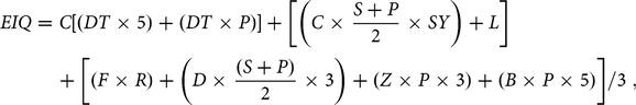 $$EIQ = C\left[ {\left( {DT \times 5} \right) + \left( {DT \times P} \right)} \right] + \left[ {\left( {C \times {{{S + P}}\over{2}} \times SY} \right) + L} \right]{\rm{\;}} + \left[ {\left( {F \times R} \right) + \left( {D \times {{{\left( {S + P} \right)}}\over{2}} \times 3} \right) + \left( {Z \times P \times 3} \right) + \left( {B \times P \times 5} \right)} \right]/3{\rm{\;}},$$
(16)
$$EIQ = C\left[ {\left( {DT \times 5} \right) + \left( {DT \times P} \right)} \right] + \left[ {\left( {C \times {{{S + P}}\over{2}} \times SY} \right) + L} \right]{\rm{\;}} + \left[ {\left( {F \times R} \right) + \left( {D \times {{{\left( {S + P} \right)}}\over{2}} \times 3} \right) + \left( {Z \times P \times 3} \right) + \left( {B \times P \times 5} \right)} \right]/3{\rm{\;}},$$
(16)
where C is chronic toxicity, DT is dermal toxicity, SY is systemicty, F is fish toxicity, L is leaching potential, R is surface loss potential, D is bird toxicity, S is soil half-life, Z is bee toxicity, B is beneficial arthropod toxicity, and P is plant surface half-life. We used the calculated field EIQFootnote
4
values as the potentially detrimental input in a DEA approach to estimate efficiency scores and EIQ slacks (our proxy for environmental inefficiency). The EIQ field-use rating is expressed as $EI{Q_{field\;use}} = EIQ \times \;AI \times \;rate\;of\;application$
.
$EI{Q_{field\;use}} = EIQ \times \;AI \times \;rate\;of\;application$
.
Although the study by Peterson and Schleier III (Reference Peterson and Schleier2014) criticized the use of EIQ in environmental impact analyses, partly because of its failure to capture environmental risk as joint probability of toxicity and exposure, the EIQ is still considered an important single index that captures various components of pollution and is therefore useful in economic analysis (Veettil, Krishna, and Qaim, Reference Veettil, Krishna and Qaim2017). It is also easy to calculate and can be adapted to different econometric model applications.
We also captured information on socioeconomic variables including education of household head, household size, age of household head, membership in a farmers’ group, and access to extension service. Farmers’ credit constraintFootnote 5 was measured as a dummy variable to capture access to credit. A number of studies have found a positive link between farmers’ access to credit and TE (e.g., Ogundari, Reference Ogundari2014; Solis, Bravo-Ureta, and Quiroga, Reference Solis, Bravo-Ureta and Quiroga2007). The descriptions, means, and standard deviations of variables are presented in Table 1. The mean age of the household head of adopters and nonadopters is about 40 years, with an average of 5 years of schooling. The reported mean schooling of both groups in our sample reflects the generally low level of education among Ghanaian farmers (Ghana Statistical Service [GSS], 2012). The average household size is about six persons, which reflects the average family size in the study area, as reported by the GSS (2012).
Table 1. Variables and descriptive statistics

Note: GHS, Ghanaian cedis; SD, standard deviation.
a Source: The online calculator https://nysipm.cornell.edu/eiq/calculator-field-use-eiq/.
3.2. Analytical strategy
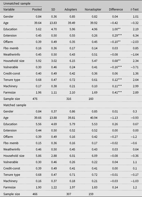
We start with propensity score matching method following Bravo-Ureta et al. (Reference Bravo-Ureta, Solis, Moreira Lopez, Maripani, Thiam and Rivas2007) and Villano et al. (Reference Villano, Bravo-Ureta, Solis and Fleming2015). First, a probit model was estimated, using observable farm and household characteristics in order to generate an adoption propensity score. Information on sociodemographic and farm characteristics was included in the probit model used for the propensity score matching. We employed the nearest neighbor matching algorithm with a maximum of five matches and caliper of 0.01. The matching procedure yielded a sample of 466 matched observations, made up of 307 adopters and 159 nonadopters, respectively. Table A1 in the Appendix presents the descriptive statistics for the matched and unmatched samples of adopters and nonadopters. As opposed to the significant differences between adopters and nonadopters in most of the variables in the unmatched sample, no significant differences in the observed characteristics are found in the matched sample, an indication that the balancing condition is satisfied (Caliendo and Kopeinig, Reference Caliendo and Kopeinig2008). The detailed description of the matching procedure and how it is applied in SPF analysis is presented in Bravo-Ureta et al. (Reference Bravo-Ureta, Solis, Moreira Lopez, Maripani, Thiam and Rivas2007) and Abdul-Rahaman and Abdulai (Reference Abdul-Rahaman and Abdulai2018).
We estimated a series of SPF models, including (1) a conventional unmatched pooled sample model with SLM adoption dummy as an independent variable, (2) a matched sample pooled model with SLM adoption as an explanatory variable,Footnote 6 and (3) two SPF models, one for adopters of SLM and one for nonadopters, using the Greene’s (Reference Greene2010) sample selection model, which corrects for selection bias from both observable and unobservable variables. Preliminary comparisons led to the rejection of the Cobb-Douglas in favor of the translog (TL) functional form.Footnote 7 The TL specification for the stochastic frontier used in our analyses is given as follows:
 $${\rm{ln}}{Y_i} = {\alpha _0} + \mathop \sum \nolimits_{k = 1}^4 {\alpha _k}{\rm{ln}}{X_{ik}} + {{1}\over{2}}\mathop \sum \nolimits_{k = 1}^4 {\alpha _{kk}}{\left( {{\rm{ln}}{X_{ik}}} \right)^2} + \mathop \sum \nolimits_{m = 1}^4 \mathop \sum \nolimits_{k = 1}^4 {\alpha _{ik}}{\rm{ln}}{X_{im}}{\rm{ln}}{X_{ik}} + \mathop \sum \nolimits_{l = 1}^2 {\beta _l}{\rm{ln}}{D_l} + {v_i} - {u_i}{\rm{\;}},$$
(17)
$${\rm{ln}}{Y_i} = {\alpha _0} + \mathop \sum \nolimits_{k = 1}^4 {\alpha _k}{\rm{ln}}{X_{ik}} + {{1}\over{2}}\mathop \sum \nolimits_{k = 1}^4 {\alpha _{kk}}{\left( {{\rm{ln}}{X_{ik}}} \right)^2} + \mathop \sum \nolimits_{m = 1}^4 \mathop \sum \nolimits_{k = 1}^4 {\alpha _{ik}}{\rm{ln}}{X_{im}}{\rm{ln}}{X_{ik}} + \mathop \sum \nolimits_{l = 1}^2 {\beta _l}{\rm{ln}}{D_l} + {v_i} - {u_i}{\rm{\;}},$$
(17)
where Yi represents output (total value of production) of the i th household; Xim , Xik is the quantity of input m or k, for m ≠ k; Dl captures dummy variables; α and β are parameters to be estimated; and vi and ui are the components of the composed error term ε. The four inputs include land cultivated, labor, capital, and herbicide, and agroecological zone dummies (Dl ) were also employed in the TL function.
The second aspect of the empirical analysis involves nonparametric estimation of environmental efficiency, which we do by estimating a DEA to obtain efficiency scores and the input slacks. We employ the procedure developed by Ji and Lee (Reference Ji and Lee2010), where we capture the four inputs (land, labor, capital, and field EIQ) and one output. Higher slacks with respect to field EIQ imply excess use of glyphosate herbicide, which might indicate environmental inefficiency (Myers et al., Reference Myers, Antoniou, Blumberg, Carroll, Colborn, Everett and Hansen2016). As indicated by Cooper, Seiford, and Tone (Reference Cooper, Seiford and Tone2007), a slacks-based measure provides a more suitable model to capture the DMU’s (farm) performance, especially if the goal is to enhance desirable output and minimize undesirable outputs and inputs.
4. Results and discussion
This section presents the results from the empirical analysis. First, we present the results of the maximum likelihood estimates of SPF models for the unmatched and matched samples. In each case, we have estimates for conventional and sample selection SPF, as well as metafrontier results. Second, the results of the TEs, TGRs, and MTEs are presented. Finally, the results of the DEA efficiency scores and herbicide-EIQ input slacks, as well as determinants of technical and environmental efficiency, are discussed.
4.1. Maximum likelihood estimates of conventional, sample selection stochastic production frontier and metafrontier models
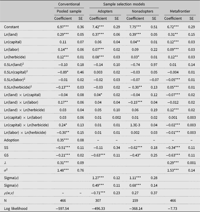
Tables 2 and 3 present the maximum likelihood estimates of separate SPF models for the unmatched and matched samples, respectively. For each table, the pooled sample estimates are presented first, sample selection SPF estimates for adopters and nonadopters of SLM are presented next, and the estimates of the metafrontier are presented last. The group sample estimates in Table 2 (unmatched sample) have been corrected for sample selectivity bias from unobservable factors, whereas their counterparts in Table 3 (matched) have been corrected for selectivity bias from both observable and unobservable factors. The inefficiency terms (sigma(u) or σ 2) in all SPF models are significant, suggesting that most of the farmers are producing below the production frontier. The sample selectivity term (ρ) for adopters is negative and statistically significant in both the unmatched and matched samples, an indication of the presence of selectivity bias from unobserved factors that lends support to the use of the sample selectivity framework to estimate the SPF (Greene, Reference Greene2010). Thus, accounting for selectivity bias is essential for unbiased and consistent TE estimates in this study (Bravo-Ureta et al., Reference Bravo-Ureta, Solis, Moreira Lopez, Maripani, Thiam and Rivas2007).
Table 2. Estimates of conventional and sample selection stochastic production frontier models: unmatched sample
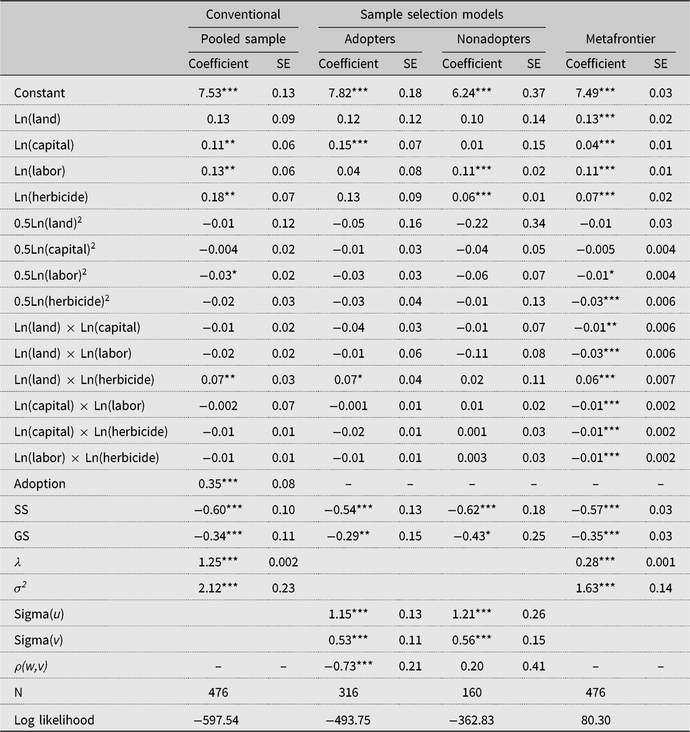
Notes: Asterisks (*, **, and ***) refer to 10%, 5%, and 1% significance levels, respectively. GS, Guinea savanna; SE, standard error; SS, Sudan savanna.
Table 3. Estimates of conventional and sample selection stochastic production frontier models: matched sample
Notes: Asterisks (*, **, and ***) refer to 10%, 5%, and 1% significance levels, respectively. GS, Guinea savanna; SE, standard error; SS, Sudan savanna.
The estimates of the probit model in the SPF selection equation are presented in Table A2 in the Appendix. The results (matched sample of Table A2) showed that extension services and ownership of machinery positively and significantly associated with farmers’ decision to adopt SLM technology, signifying the role of extension access in technology adoption as observed in earlier studies (e.g., Solis, Bravo-Ureta, and Quiroga, Reference Solis, Bravo-Ureta and Quiroga2007). Farmers’ perceived vulnerability to drought based on experience also significantly influenced their decision to adopt SLM technology, a finding that is consistent with the study by Ainembabazi and Mugisha (Reference Ainembabazi and Mugisha2014) in Uganda. As noted earlier, we focus our discussions concerning the SPF results on the matched sample in Table 3.
The coefficients of the first-order terms for most of the inputs representing partial elasticities are positive and significant, implying that these inputs contribute to moving farm productivity to the frontier. It is important to note that the coefficient of herbicide, the input that contains the environmentally detrimental active ingredient (glyphosate), is positive in most of the SPF models, especially in Table 3. This implies that the use of herbicides is positively correlated with increased productivity. It is also important to mention that farmers in the transitional agroecological zone (the reference location) are likely to be more productive compared with their counterparts in the Sudan savanna or Guinea savanna agroecological zones, signifying the relevance of capturing agroecological zone differences in specifying agricultural production functions (Solis, Bravo-Ureta, and Quiroga, Reference Solis, Bravo-Ureta and Quiroga2007). Apart from capturing climatic effects, the agroecological zone differences may also capture unmeasured location-specific institutional differences that may influence productivity.
4.2. Technical efficiency and technology gap ratios
Table 4 presents the TE scores and TGR obtained from the estimated sample-selectivity SPF and metafrontier models. In the unmatched sample, the TE estimate for adopters (55%) appears to be significantly higher than that of nonadopters (49%). However, there appears to be no difference between adopters and nonadopters in the matched sample (that is 47% and 46% for adopters and nonadopters, respectively). To make a more reasonable comparison across groups, a metafrontier regression was estimated, using Huang, Huang, and Liu’s (Reference Huang, Huang and Liu2014) approach, and the gaps between the metafrontier and the individual group frontiers (TGRs) were derived, with higher TGRs indicating better returns from technology. The MTE was then calculated. The results (Table 4, matched sample) indicate that the average TGR for adopters is about 0.95, ranging from 0.63 to 1. However, the TGR among nonadopters ranges from 0.14 to 0.98, with an average of 0.88.
Table 4. Technical efficiency scores with the estimated models
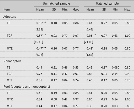
Notes: Asterisks (*, **, and ***) refer to 10%, 5%, and 1% significance levels, respectively. MTE, technical efficiency with respect to the metafrontier; SD, standard deviation; TE, technical efficiency; TGR, technological gap ratio.
In the unmatched sample, the MTE scores for adopters and nonadopters of SLM technology are 47% and 38%, respectively. However, the MTE scores indicate that on average, SLM technology farms are about 43% technically efficient, and the non-SLM technology farms are 40% technically efficient. This implies that with respect to the matched sample, adoption of SLM technology tends to increase TE by 7.5% among adopters compared with nonadopters. Although the differences in TE between adopters and nonadopters appear marginal (and significant at the 10% level), our results are still consistent with previous findings and field reports of the positive impact of SLM on farm performance (Zougmore, Jalloh, and Tioro, Reference Zougmore, Jalloh and Tioro2014). Farmers who shift from conventional farming to SLM practices might be the ones with higher managerial abilities and who are also more environmentally conscious. To show how the two groups perform in terms of expected farm revenues, we predicted and compared their frontier outputs for both unmatched and matched samples (Table 5). The results showed that adopters performed better in terms of expected farm revenues with much higher performance coming from the matched sample, confirming the output enhancement potential of the SLM technology.
Table 5. Predicted frontier of log farm revenues of adopters and nonadopters In unmatched and matched samples

Notes: Asterisks (*, **, and ***) refer to 10%, 5%, and 1% significance levels, respectively. The t-statistic is based on the mean difference between the predicted frontiers of adopters and nonadopters. ATT, average treatment effect on the treated.
4.2.1. Data envelopment analysis technical efficiency and input slacks among adopters and nonadopters
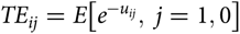
The distribution of the DEA TE scores are shown in Table A3 in the Appendix. The results confirm that adopters generally obtain higher efficiency scores than nonadopters. The TE scores of the pooled sample appear to be normally distributed, but the distributions are negatively skewed among adopters and nonadopters, with a higher number of adopters (42%) compared with 36% of nonadopters obtaining efficiency scores of 60% to 80%. The DEA analysis also reveals the existence of slacks in some inputs. Because a slack indicates excess of an input, a farm household can reduce its use of an input by the quantity of slack without reducing its output. From Figure 1, it is obvious that adopters and nonadopters make excess use of herbicides (excess field EIQ) at an average of 57% and 26%, respectively. Because excess use of herbicides has environmental implications, we discuss the determinants of TE and environmental efficiency (excess EIQ) in the next section.
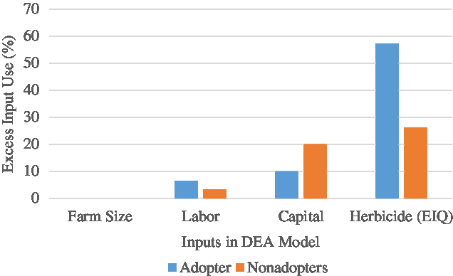
Figure 1. Input slacks from data envelopment analysis (DEA) model by adoption status.
4.2.2. Determinants of technical and environmental efficiency
In the context of policy, it is more useful to determine what influences efficiency/inefficiency (i.e., the variables to which TE and environmental inefficiency are related). Thus, the DEA scores were regressed on specific household socioeconomic characteristics, using the FRMs, following the example of recent studies (e.g., Abdulai and Abdulai, Reference Abdulai and Abdulai2017; Ogundari, Reference Ogundari2014; Ramalho, Ramalho, and Henriques, Reference Ramalho, Ramalho and Henriques2010). We report the specification of the test statistic for each of the FRMsFootnote 8 (logit, probit, loglog, and cloglog). All the models of the FRM (with respect to the TE scores) show similar test statistics, indicating that all the competing models fit out data (Ramalho, Ramalho, and Henriques, Reference Ramalho, Ramalho and Henriques2010). Based on the RESET test for misspecification, we discuss the determinants of DEA efficiency scores using the cloglog specification (Table 6). The estimates reveal that TE scores are significantly influenced by adoption status, credit access, extension access, and household size. On the other hand, environmental inefficiency appears to also be influenced by adoption of SLM, credit access, and usufruct right/tenure security.
Table 6. Determinants of technical efficiency and environmental inefficiency (excess EIQ)

Notes: Asterisks (*, **, and ***) refer to 10%, 5%, and 1% significance levels, respectively. EIQ, environmental impact quotient; SE, standard error.
a The statistic used to assess misspecification is the Ramsey test, RESET test.
b In the matched sample, the analysis was restricted to only farmers who applied glyphosate herbicide, because they are the only farmers expected to have excess EIQ in our context.
Adoption is positively associated with DEA TE scores, confirming the results of the SPF analysis discussed previously. This finding is in-line with the results reported by Khanal et al. (Reference Khanal, Clevo, Boon and Viet-Ngu2018), who found that adoption of soil and water conservation practices by households in Nepal resulted in improved farm efficiency. However, the positive correlation between adoption of SLM and environmental inefficiency (excess EIQ) implies that adoption of some SLM practices (e.g., minimum/zero tillage) may be associated with the use of higher levels of herbicides to control weeds and to ensure minimum soil disturbance. Although our finding is not able to indicate the threshold EIQ level that is considered environmentally unsustainable, our results confirm the concern about the increasing levels of glyphosate use in crop production, especially in zero-tillage practices (Myers et al., Reference Myers, Antoniou, Blumberg, Carroll, Colborn, Everett and Hansen2016). Some recent studies propose the use of weed suppressing crops, cover cropping, and mixed cropping to minimize the dependence on herbicides for weed control in SLM and soil conservation systems (Price and Norsworthy, Reference Price and Norsworthy2013).
The results also show a positive and significant relationship between extension access and TE, but not in the environmental efficiency models, suggesting that farmers with lower extension contacts tend to be less efficient. Although education has the expected sign in both the TE and environmental efficiency models, the estimates are only statistically significant in the environmental efficiency model, particularly in the cloglog model. The estimate for household size is positive and statistically significant, implying that efficiency of farms could be associated with family size. In a meta-analysis of efficiency studies in Africa, Ogundari (Reference Ogundari2014) reported that 22% of increase in technical efficiency was attributed to household size.
In addition, the results reveal a negative and significant relationship between the variable representing credit constraint and technical efficiency, suggesting that credit-constrained farmers tend to be less efficient, a finding that is consistent with other studies in SSA countries (Abdulai and Huffman, Reference Abdulai and Huffman2000; Ogundari, Reference Ogundari2014). The findings are also in-line with the assertion that enhancing farmers’ access to credit could significantly improve agricultural productivity and output, as well as help reduce food insecurity in SSA countries (Lee, Reference Lee2005). The estimate of farmland usufruct right/tenure security is positive and significant in the environmental efficiency models, implying that tenure security (longer usufruct right) may be associated with higher field EIQ. This may appear strange, but possible, given the fact that farmers with tenure security are usually the ones who will be prepared to invest in SLM including practices that may involve the use of more herbicides. Because of data limitations, the present study is unable to establish whether organic manure generated through SLM practices that use herbicides is sufficient to speed up the breakdown of glyphosate into nontoxic components (Williams et al., Reference Williams, Aardema, Acquavella, Berry, Brusick, Burns and de Camargo2016). If this scenario holds, as suggested by Williams and others, then adoption of SLM, even with the use of Roundup herbicides, will positively influence the quality of arable lands.
5. Conclusions
In this study, we examined the impact of adoption of SLM on technical and environmental efficiency among smallholder farmers in Ghana. The empirical results revealed that SLM technology farmers are technically more efficient than conventional technology farmers, implying that SLM has the potential to reduce the economic drain. The metafrontier estimates also showed that SLM technology adopters are 7.5% more technically efficient than the nonadopters. Apart from adoption of SLM technology, the results revealed other key drivers of efficiency levels of smallholder food crop farmers to be credit access, extension service, and land tenure security. The results also showed that adoption of SLM positively and significantly influenced excess EIQ, which might have environmental implications.
Overall, the findings suggest that the potential role of agriculture in achieving national food security, eradicating poverty, and reducing unemployment could be enhanced if policy actions are undertaken to address problems associated with the identified drivers of farmers’ efficiency. In addition, the findings indicate that while government and other agencies focus on promoting production technologies that will enhance land use sustainability and fertility, there is the need for caution about potential harmful effects of excess herbicides, particularly glyphosates that are used with some SLM practices. For instance, promotion of non-herbicide-based SLM practices such as crop rotation and cover crops or the use of weed-suppressive crop varieties should be encouraged to minimize the use of herbicides among farmers. Moreover, intensifying farmer education through enhanced extension services should also be encouraged. Furthermore, improving access to credit will help improve food crop farmers’ efficiency levels and help improve food productivity. However, further research is required to determine whether organic manure generated through SLM practices that rely on herbicides, such as zero tillage or conservation agriculture, is sufficient to facilitate the decomposition of glyphosate into nontoxic components.
Supplementary material
To view supplementary material for this article, please visit https://doi.org/10.1017/aae.2019.34
Acknowledgments
The authors acknowledge financial support by the University of Kiel Library within the funding program of the State of Schleswig Holstein Open Access Publications Funds. The first author also acknowledges the funding support of the DAAD (Deutcsher Akademischer Austauschdienst) for his PhD studies.
Appendix
Table A1. Summary statistics of variables for matched and unmatched samples
Note: Asterisks (*, **, and ***) refer to 10%, 5%, and 1% significance levels, respectively.
Table A2. Estimates of the probit selection equation using unmatched and matched samples
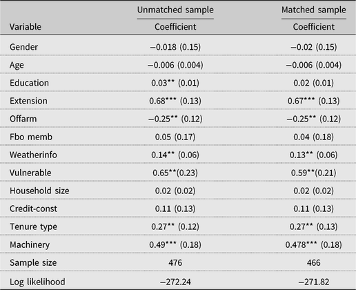
Notes: Asterisks (*, **, and ***) refer to 10%, 5%, and 1% significance levels, respectively. Values in parentheses are standard errors.
Table A3. Distribution of efficiency scores by adoption status


 Open access