


1. Introduction
Ice-sheet surface elevation responds to a variety of time-varying subglacial phenomena, including subglacial-lake volume change, basal-drag variations, and melting or freezing at the ice-water interface. Active subglacial lakes (i.e., those that experience observable volume change in the observational record) in particular have received much attention due to the localized perturbations they produce in ice-sheet surface elevation during volume-change events (e.g., Gray and others, Reference Gray2005; Wingham and others, Reference Wingham, Siegert, Shepherd and Muir2006; Fricker and others, Reference Fricker, Scambos, Bindschadler and Padman2007). NASA's Ice, Cloud, and land Elevation Satellite (ICESat) mission (2003-2009) and the European Space Agency's CryoSat-2 satellite altimetry mission (2010-present) facilitated the detection of over one hundred active subglacial lakes beneath the Antarctic Ice Sheet (e.g., Smith and others, Reference Smith, Fricker, Joughin and Tulaczyk2009; Wright and Siegert, Reference Wright and Siegert2012; Fricker and others, Reference Fricker, Siegfried, Carter and Scambos2016; Livingstone and others, Reference Livingstone2022), driving investigations into their possible relation to fast ice flow (e.g., Stearns and others, Reference Stearns, Smith and Hamilton2008; Scambos and others, Reference Scambos, Berthier and Shuman2011; Siegfried and others, Reference Siegfried, Fricker, Carter and Tulaczyk2016) and into their ability to host microbial ecosystems (e.g., Christner and others, Reference Christner2014; Achberger and others, Reference Achberger2016; Davis and others, Reference Davis2023). Fewer subglacial lakes have been discovered beneath the Greenland Ice Sheet based on ice-surface changes, suggesting that there may be significant differences in subglacial hydrological conditions there relative to the Antarctic Ice Sheet (e.g., Bowling and others, Reference Bowling, Livingstone, Sole and Chu2019; Livingstone and others, Reference Livingstone2019, Reference Livingstone2022).
High-resolution satellite altimetry data from NASA's ICESat-2 mission (2018-present) presents a valuable opportunity to continue investigating dynamic conditions and constraining water budgets beneath ice sheets (e.g., Markus and others, Reference Markus2017; Neckel and others, Reference Neckel, Franke, Helm, Drews and Jansen2021; Siegfried and Fricker, Reference Siegfried and Fricker2021). ICESat-2's temporal resolution (91 day repeat cycle) and spatial resolution (~3.3 km across-track between beam pairs and ~90 m between beams within the pairs) provide unprecedented coverage of active subglacial lakes, which are typically greater than ~10 km in diameter and fill or drain over multiple years (Smith and others, Reference Smith, Fricker, Joughin and Tulaczyk2009; Siegfried and Fricker, Reference Siegfried and Fricker2021; Stubblefield and others, Reference Stubblefield, Creyts, Kingslake, Siegfried and Spiegelman2021a). Modeling has shown that accurately estimating subglacial-lake volume change, areal extent, and highstand or lowstand timing from altimetry alone can be complicated by the effects of viscous ice flow (Stubblefield and others, Reference Stubblefield, Creyts, Kingslake, Siegfried and Spiegelman2021a). Basal vertical velocity anomalies associated with subglacial lake activity can manifest with a wider areal extent and smaller amplitude at the ice-sheet surface when ice flows laterally toward or away from the lake during volume-change events. Ice viscosity, ice thickness, and basal drag exert strong control on ice flow and, therefore, also influence the surface expression of subglacial lake activity (Stubblefield and others, Reference Stubblefield, Creyts, Kingslake, Siegfried and Spiegelman2021a). Although satellite altimetry data has been incorporated in basal-drag inversions (e.g., Larour and others, Reference Larour2014; Arthern and others, Reference Arthern, Hindmarsh and Williams2015; Goldberg and others, Reference Goldberg, Heimbach, Joughin and Smith2015; Mosbeux and others, Reference Mosbeux, Gillet-Chaulet and Gagliardini2016), inverse methods that quantify subglacial-lake activity from altimetry and account for ice-flow effects have not yet been developed.
Inversion of time-varying altimetry data necessitates leveraging reduced-order models to alleviate the computational cost associated with repeatedly solving the forward problem. Dimensionality reduction is often achieved using ice-flow models that are based on depth-integrated approximations of the Stokes equations (e.g., Greve and Blatter, Reference Greve and Blatter2009). Solving the linearized Stokes equations on simplified domains with spectral methods is an alternative way to achieve computational efficiency when the full stresses in the ice must be resolved (e.g., Budd, Reference Budd1970; Hutter and others, Reference Hutter, Legerer and Spring1981; Balise and Raymond, Reference Balise and Raymond1985; Gudmundsson, Reference Gudmundsson2003; Sergienko, Reference Sergienko2012). Previous inversions relying on perturbation methods have not included time-varying data (Gudmundsson and Raymond, Reference Gudmundsson and Raymond2008; Thorsteinsson and others, Reference Thorsteinsson2003). Likewise, a computational method for inverting time-varying elevation data with perturbation-based models would be a valuable step toward quantifying time-varying subglacial lake perturbations. We use this small-perturbation approach as subglacial lake activity typically only induces small perturbations in ice-surface elevation (e.g., a few meters) relative to ice thickness.
Here, we derive, test, and apply an altimetry-based inverse method for quantifying basal vertical velocity perturbations that arise from subglacial lake activity. First, we outline the forward model for the perturbation in ice-surface elevation that is produced by a basal vertical velocity forcing. We then derive the inverse method from a least-squares optimization problem. To verify and validate the method, we present tests with synthetic data from both the linearized and nonlinear models. We then apply the method to a collection of active subglacial lakes in Antarctica (Fig. 1). The results show that ice flow can produce significant discrepancies between the inverse method and a traditional altimetry-based estimation method for calculating changes in subglacial water volume over the current ICESat-2 time period. We conclude by discussing limitations, extensions, and further applications of the method.

Figure 1. Map of ICESat-2 ATL15 gridded product (Smith and others, Reference Smith2022) showing the elevation change of the Antarctic Ice Sheet between October 2018 and April 2022. The map-plane (x, y) coordinates in the ATL15 dataset correspond to the Antarctic Polar Stereographic Projection (EPSG:3031). Insets show the locations of the subglacial lakes targeted as examples in this study. Subglacial lake boundaries derived from surface altimetry are shown as gray lines (Siegfried and Fricker, Reference Siegfried and Fricker2018). Regional thinning occurs around Thwaites Lake 170 (Thw170) and regional thickening occurs around Mercer Subglacial Lake (SLM). Regional elevation-change trends around Slessor Glacier (lake Slessor23), MacAyeal Ice Stream (lake Mac1), and Byrd Glacier (lake Byrds10) are less pronounced. We remove regional trends to produce elevation-change anomalies that are used in the inversions.
2. Method
In this section, we derive the forward model and the associated inverse method. First, we outline the general Stokes flow problem to highlight the governing equations and simplifying assumptions. Then, we outline a derivation of the small-perturbation model that is used in the inverse method. Finally, we derive the inverse method with a least-squares optimization approach.
2.1. Stokes flow
We assume that ice deforms as a viscous fluid according to the incompressible Stokes equations, which are given by


where ρ i is the ice density, $\pmb {u} = [ u,\; \, v,\; \, w] ^{\rm T}$ is the ice velocity, and $\pmb {g} = g[ 0,\; \, 0,\; \, -1] ^{\rm T}$
 denotes gravitational acceleration with magnitude g = 9.81 m s−2 (Greve and Blatter, Reference Greve and Blatter2009; Stubblefield and others, Reference Stubblefield, Spiegelman and Creyts2021b). We have excluded possible elastic components of ice deformation by assuming a viscous rheology and revisit this choice in the discussion. The stress tensor $\pmb {\sigma }$
 is defined via

where p is the pressure, ${\sf I}$ is the identity tensor, and η is the viscosity. At the ice-bed boundary we assume a sliding law of the form

where β is the basal drag coefficient, $\pmb {n}$ is an outward-pointing unit normal to the boundary, and ${\sf T} = {\sf I} - \pmb {n}\pmb {n}^{\rm T}$
 is a projection tangential to the ice-sheet surface (Stubblefield and others, Reference Stubblefield, Spiegelman and Creyts2021b). Although the small-perturbation model used in the inversions assumes a Newtonian viscosity and linear sliding law (i.e., constant η and β), we will also consider synthetic data produced by a fully nonlinear model with Glen's law viscosity (Glen, Reference Glen1955) and a nonlinear Weertman-style sliding law (Weertman, Reference Weertman1957) to test the validity of these simplifications.
The upper surface of the ice-sheet z = h(x, y, t) evolves over time according to the kinematic equation

where the velocity components are evaluated at the surface (z = h). We assume that a stress-free condition,

holds at the upper surface of the ice sheet. We approximate the spatial domain as a horizontally unbounded slab because the ice-sheet extent is much greater than areal extent of the subglacial lakes. Away from the lake, we assume that all quantities approach an appropriate far-field reference state that is based on data and available ice-sheet model output.
2.2. Small-perturbation model
Now we will describe the forward model that is used in the inverse method. Although small-perturbation models have been derived previously, we outline a derivation here to highlight the assumptions underlying the inverse method (Balise and Raymond, Reference Balise and Raymond1985; Gudmundsson, Reference Gudmundsson2003). Our goal is to find the basal vertical velocity perturbation w b that produces the surface elevation-change anomaly Δh a under the assumption that these anomalies arise from subglacial lake activity (Fig. 2). We could also incorporate a basal drag anomaly to represent a slippery spot over a lake in the small-perturbation framework (e.g., Gudmundsson, Reference Gudmundsson2003; Stubblefield, Reference Stubblefield2022), but the resulting dipolar elevation-change anomaly (Sergienko and others, Reference Sergienko, MacAyeal and Bindschadler2007) is not discernible in any of the active lakes considered herein. We revisit this idea in the discussion.

Figure 2. Sketch of linearized model setup. The horizontal (map-plane) coordinates are (x, y) with the y direction pointing into the page. The basal vertical velocity anomaly w b produces an elevation-change anomaly Δh a. The ice thickness is $\bar {H}$ and the horizontal surface velocity is $\bar {\pmb {u}}$
 in the reference flow state. The ice flow is aligned with the x axis here for simplicity but generally also has a component in the y direction. The volume change estimated from the elevation-change anomaly Δh a can deviate significantly from the subglacial water-volume change (Stubblefield and others, Reference Stubblefield, Creyts, Kingslake, Siegfried and Spiegelman2021a).
To derive a simplified model for this system, we assume that Δh a and w b are small perturbations from a known reference state that is (approximately) characterized by a constant ice thickness $\bar {H}$ , horizontal surface velocity $\bar {\pmb {u}} = [ \bar {u},\; \, \bar {v}] ^T$
 , ice viscosity $\bar {\eta }$
 , and basal drag coefficient $\bar {\beta }$
 . We further assume that the basal surface is horizontal in the reference state and that the ice pressure equals the cryostatic pressure. Strictly speaking, an advective component is only present in the free-slip limit ($\bar {\beta } = 0$
 ) under the assumption of a horizontally uniform Stokes flow over a flat bed subject to the stress boundary conditions (4) and (6). However, we retain a background advective velocity in all cases for consistency with the data.
Letting [u h, v h, w h]T denote the perturbation in ice-sheet surface velocity, we insert perturbations to the reference states, $h = \bar {H} + \Delta h_{\rm a}$ and $\pmb {u} = [ \bar {u},\; \, \bar {v},\; \, 0] ^T + [ u_h,\; \, v_h ,\; \, w_h] ^T$
 , into the kinematic equation (5) to obtain

We have neglected terms involving products of perturbations in (7) under the assumption of small perturbations. We solve equation (7) by taking Fourier transforms with respect to the horizontal coordinates (x, y) to obtain

where $\pmb {k} = [ k_x,\; \, k_y] ^{\rm T}$ is the horizontal wavevector. The vertical surface velocity is assumed to satisfy the Stokes flow problem (1)–(6), subject to the above simplifications, which allows us to derive a closed-form expression of the solution operator (Balise and Raymond, Reference Balise and Raymond1985; Gudmundsson, Reference Gudmundsson2003; Stubblefield and others, Reference Stubblefield, Creyts, Kingslake, Siegfried and Spiegelman2021a).
We algebraically solve the Fourier-transformed Stokes problem to obtain an expression for the transformed vertical surface velocity,

in terms of the basal vertical velocity and surface elevation anomalies (e.g., Stubblefield and others, Reference Stubblefield, Creyts, Kingslake, Siegfried and Spiegelman2021a, Supporting Information). In Eqn. (9), ${\cal R}$ is a relaxation function that controls the decay rate of the elevation anomaly, and ${\cal T}$
 is a transfer function that maps the basal vertical velocity anomaly to its surface expression. These functions depend on the scaled wavevector magnitude $k' = \vert \pmb {k}\vert \bar {H}$
 and drag coefficient $\gamma = {\bar {\beta } \bar {H}} / ( {2\bar {\eta } k'} )$
 through the relations

and

For a detailed derivation of the expressions (10) and (11) see, for example, Stubblefield and others (Reference Stubblefield, Creyts, Kingslake, Siegfried and Spiegelman2021a, Supporting Information) and Stubblefield (Reference Stubblefield2022, Appendix E).
Substituting the expression (9) into (8), we find that the ice-surface elevation anomaly Δh a evolves in frequency space via

The solution to equation (12) is given by

where * denotes convolution over time and Δh 0 is the elevation perturbation at the initial time t = 0. The kernel ${\cal K}$ , defined by

controls the decay of the elevation-change anomaly and transfer of the basal anomaly to the surface. The characteristic time scale for the decay of surface-elevation anomalies is

which controls the magnitude of the relaxation function ${\cal R}$ (cf. Turcotte and Schubert, Reference Turcotte and Schubert2014, Chapter 6). The effects of viscous ice flow influence the surface expression of lake activity when the viscous relaxation time t relax is comparable to the lake filling or draining timescale (Stubblefield and others, Reference Stubblefield, Creyts, Kingslake, Siegfried and Spiegelman2021a). We highlight the importance of the viscous relaxation time in the examples below.
2.3. Inverse method
Now we will outline the inverse method. We let ${\sf F}$ denote the (map-plane) Fourier transform operator and define the relative elevation-change anomaly via

which has the contribution from the initial value in equation (13) removed. From equation (13), we define the operator ${\sf G}$ that maps w b to the relative elevation change d via

where the kernel ${\cal K}$ is defined in equation (14).
We consider a regularized least-squares objective functional,

where t f is the final time and the parameter $\varepsilon$ controls the strength of the regularization term. While the regularization in (18) promotes smoothness, other regularizations could be chosen to promote sparsity of the basal forcing, for example (Stadler, Reference Stadler2009). The minimizer of the objective (18) satisfies the normal equation

which can be derived with variational calculus (Vogel, Reference Vogel2002; Hanke, Reference Hanke2017). The adjoint operator ${\sf G}^\ast$ in (19) is given by

for any function f, where $\star$ denotes cross-correlation over time.
We solve the equation (19) with the conjugate gradient method to obtain the basal vertical velocity w b. In using the conjugate gradient method to solve this operator equation, we avoid explicitly constructing matrices corresponding to the forward and adjoint operators, and instead simply require the action of these operators on functions (Atkinson and Han, Reference Atkinson and Han2009, Section 5.6). We implemented the discretized inverse method in Python with SciPy's fast Fourier transform and convolution algorithms (Virtanen and others, Reference Virtanen2014). The code is openly available (https://doi.org/10.5281/zenodo.8371416).
2.4. Estimation of water-volume change
To compare the inversion with previous estimation methods, we will focus on estimating subglacial water-volume changes. Given the basal vertical velocity inversion w b, the basal water-volume change over a map-plane area B can be computed via

Alternatively, the volume-change has often been estimated in previous studies by integrating the elevation change anomaly over the static outline of a lake (Fricker and Scambos, Reference Fricker and Scambos2009; Smith and others, Reference Smith, Fricker, Joughin and Tulaczyk2009). Using this approach, the water-volume change is estimated by

where we have integrated over the same map-plane area B. Although an alternative lake boundary could be identified with the inversion, we use the same boundary to calculate both estimates for consistency in comparison. We revisit this problem in the discussion.
In the limits ${\cal R}\to 0$ and ${\cal T}\to 1$
 , equation (12) implies that these volume changes are equivalent (i.e., ΔV inv = ΔV alt). This “rigid-ice” limit is approached when the ice is viscous enough for the relaxation timescale, t relax (eq. (15)), to greatly exceed the volume-change timescale (Stubblefield and others, Reference Stubblefield, Creyts, Kingslake, Siegfried and Spiegelman2021a). Although incompressibility causes these volume changes to be equal when integrating over the entire areal extent of a glacier, this approach is impractical for the Antarctic Ice Sheet due to the presence of multiple lakes and regional thickening or thinning trends. We explore the discrepancy between the inversion-derived estimate (21) and surface-derived estimate (22) for a range of parameters in the examples below.
3. Synthetic examples
Before applying the method to the ICESat-2 altimetry data, we first solve two problems with synthetic data to validate the method and illustrate the range of behaviors found in the ICESat-2 examples below. First, we verify the implementation by inverting synthetic data that is produced by prescribing the linearized model with a known basal vertical velocity field and then adding Gaussian white noise to the resulting elevation change. For consistency with the ICESat-2 examples, we remove a small off-lake elevation-change component, Δh off, from the elevation change as detailed in the next section. For this example, we choose a basal vertical velocity field that is a Gaussian bump undergoing sinusoidal oscillations in time. The inverse method is able to reconstruct the basal vertical velocity and volume-change time series from the synthetic data (Fig. 3). We find that there is little deviation ($\lesssim 5\%$ ) between the volume-change estimates (21) and (22) on short timescales (i.e., less than ~2.5 years), whereas large deviations occur over decadal timescales. This behavior arises because the viscosity is $\bar {\eta } = 10^{15}$
 Pa s for this example, leading to characteristic relaxation timescale of t relax ≈ 2.8 yr. These results highlight that there will not be significant deviations between the altimetry-based and inversion-based volume-change estimates over the current ICESat-2 time period if the ice viscosity reaches this magnitude. We provide an example of this behavior below. In all examples herein, we set the regularization parameter to $\varepsilon = 1$
 in equation (19), which results in accurate reconstructions of the synthetic examples without over-fitting the data.
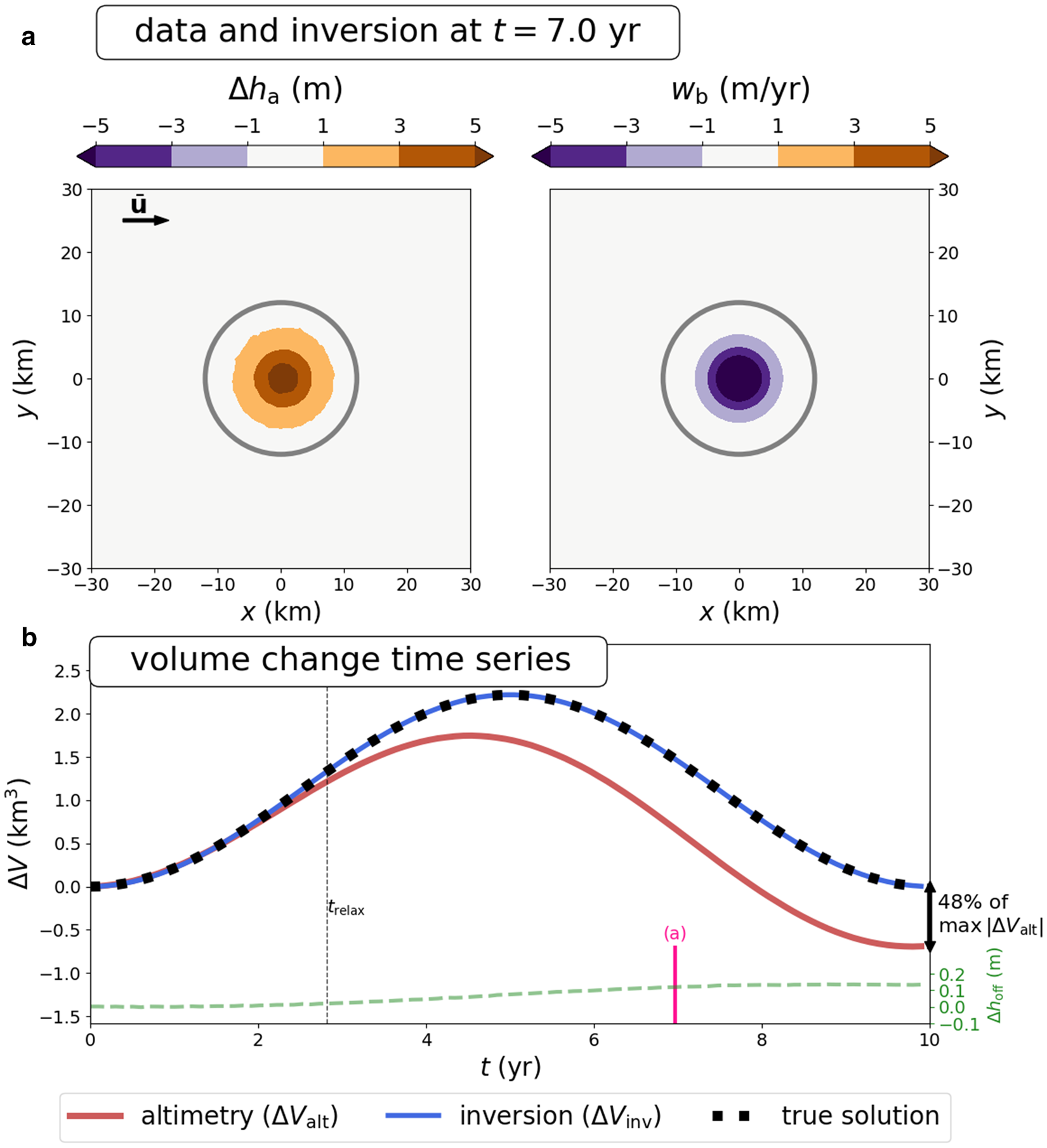
Figure 3. Inversion results for synthetic data produced with the linearized model. (a) Map-plane elevation anomaly and inversion at t = 7 yr. (b) Time series of the surface-derived volume change (ΔV alt), the inversion-based volume change (ΔV inv), and the off-lake component (Δh off) that is removed prior to inversion. The gray contours in (a) and (b) show the boundaries used to compute the volume-change time series. The ice flow direction is shown by the black arrow in (a). The maximum deviation between the surface-derived volume change and the inversion in (b) is 0.83 km3, or 48% of the maximum amplitude of the surface-derived estimate. The inversion accurately recovers the true water-volume change (dashed black line). The parameters for this example are $\bar {H} = 2500$ m, $\bar {\eta } = 10^{15}$
 Pa s, $\bar {\beta } = 10^{11}$
 Pa s m−1, $\bar {u} = 200$
 m yr−1, and $\bar {v} = 0$
 m yr−1. The viscous relaxation time associated with these parameters is t relax = 2.82 yr. The pink line marks the time step shown in (a). See Movie S1 for an animation of the inversion over all time steps.
Next, we show an example with synthetic data produced by a fully nonlinear model to test the assumptions underlying the small-perturbation approach (Stubblefield and others, Reference Stubblefield, Spiegelman and Creyts2021b, Reference Stubblefield, Creyts, Kingslake, Siegfried and Spiegelman2021a). The nonlinear model assumes a Glen's law viscosity (Glen, Reference Glen1955; Cuffey and Paterson, Reference Cuffey and Paterson2010), a nonlinear Weertman-style sliding law (Weertman, Reference Weertman1957), fully nonlinear surface kinematic equations, and vanishing basal drag over the lake. For this example, we have assumed radial symmetry with respect to the map-plane coordinates (x, y) to facilitate numerical solution in three spatial dimensions. We also prescribe a more complex volume-change time series with a duration of three years in accordance with the current ICESat-2 time span and choose a lower viscosity for this example, $\bar {\eta } = 10^{14}$ Pa s (Fig. 4). Despite the simplifications inherent to the inverse method, the inversion accurately recovers the volume change time series that is produced by the nonlinear model (Fig. 4). Most importantly, the inversion is much more accurate than the surface-based volume change for this parameter regime. This example shows that ice viscosities on the order of $\bar {\eta } = 10^{14}$
 Pa s can result in significant volume-change deviations over the current ICESat-2 time span. In particular, the examples in Figure 3 and Figure 4 show that the altimetry-based estimate tends to underestimate the magnitude of the true water volume change, regardless of whether the volume change is positive or negative. Next, we describe the data and preprocessing steps before discussing examples of ICESat-2 inversions.
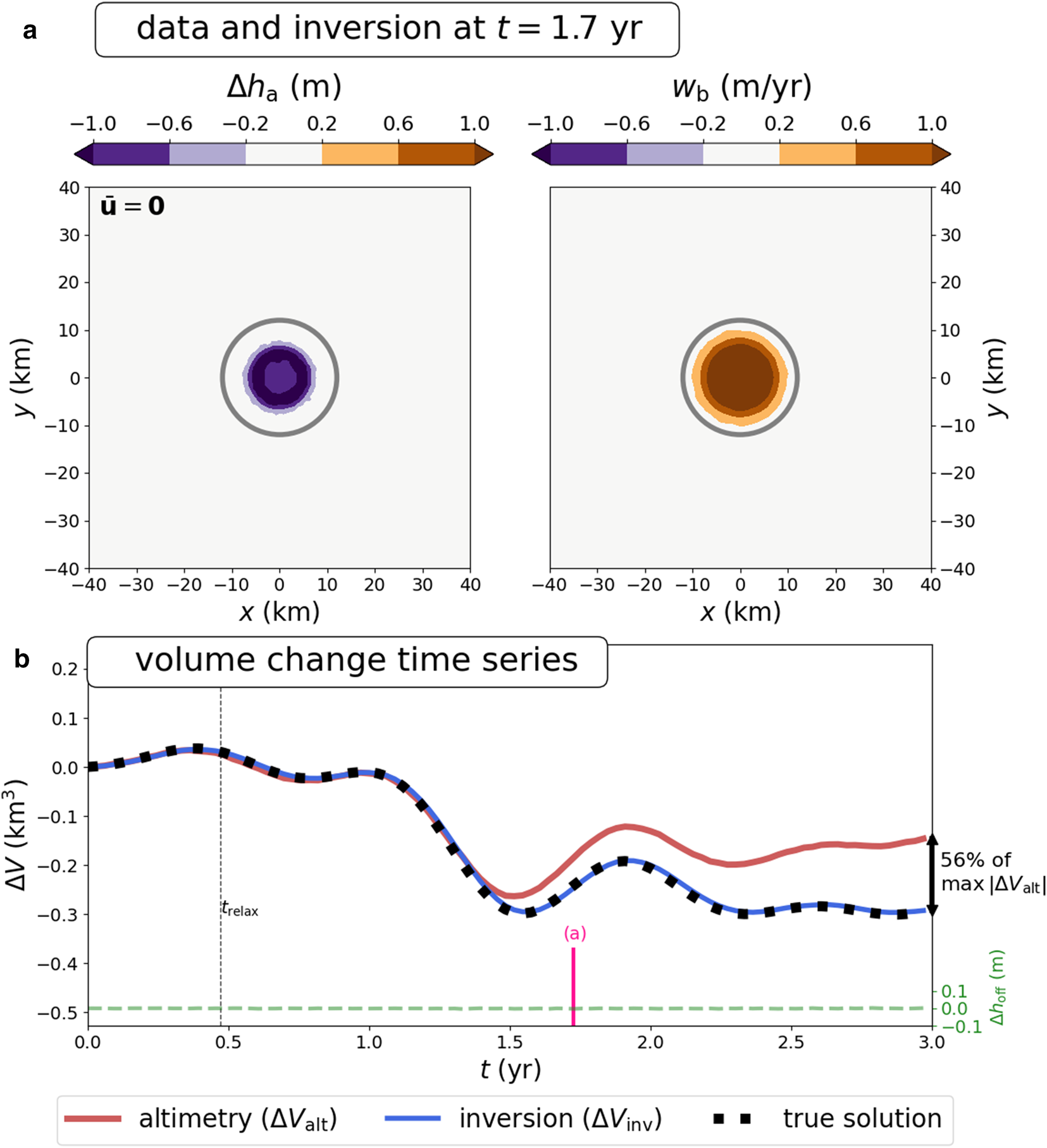
Figure 4. Inversion results for synthetic data produced with a radially-symmetric nonlinear Stokes model (Stubblefield and others, Reference Stubblefield, Spiegelman and Creyts2021b). (a) Map-plane elevation anomaly and inversion at t = 1.7 yr. (b) Time series of the surface-derived volume change (ΔV alt), the inversion-based volume change (ΔV inv), and the off-lake component (Δh off) that is removed prior to inversion. The gray contours in (a) and (b) show the boundaries used to compute the volume-change time series. The maximum deviation between the surface-derived volume change and inversion in (b) is 0.15 km3, or 56% of the maximum amplitude of the surface-derived estimate. The inversion accurately recovers the true water-volume change (dashed black line). The parameters for this example are $\bar {H} = 1500$ m, $\bar {\eta } = 10^{14}$
 Pa s, $\bar {\beta } = 10^{10}$
 Pa s m−1, $\bar {u} = 0$
 m yr−1, and $\bar {v} = 0$
 m yr−1. The viscous relaxation time associated with these parameters is t relax = 0.47 yr. The pink line marks the time step shown in (a). See Movie S2 for a detailed animation of the nonlinear model and Movie S3 for an animation of the inversion over all time steps.
4. Data and preprocessing
We use the ICESat-2 ATL15 L3B Gridded Antarctic and Arctic Land Ice Height Change (Version 2) data product (Smith and others, Reference Smith2022) to obtain elevation-change anomalies above the Antarctic subglacial lakes shown in Figure 1. The map-plane (x, y) coordinates in the ATL15 dataset correspond to the Antarctic Polar Stereographic Projection based on the WGS-84 ellipsoid (EPSG:3031). For the examples explored here, we interpolated the ICESat-2 ATL15 data onto a space-time grid with 100 points in each direction (t, x, y) to obtain the same resolution as the numerical model. Alternatively, we could restrict the model-data misfit in (18) to the discrete set of data points, but this could require additional temporal regularization that we have not included in this study. We remove any regional thickening or thinning trends by subtracting the spatially averaged off-lake component, Δh off, as described below. We also have to establish a reference elevation profile to define the elevation-change anomaly. By default, the elevation changes in ATL15 are relative to the ice-surface elevation on January 1, 2020. In general, the elevation anomaly can be defined relative to any of the ATL15 time points by subtracting the elevation surface at a particular reference time t ref. Therefore, the elevation change anomaly is derived from the ATL15 elevation change product Δh via

where Δh off is the (time-varying) spatial average of Δh away from the lake. Here, the spatial average is taken over all points that are at a distance greater than $80\%$ from the centroid of the lake to the boundary of the computational domain.
Based on previously identified lake activity, an appropriate reference time t ref to define the anomalies happens to be the initial time in the ATL15 product, October 1, 2018, for all of the lakes considered here except Mercer Subglacial Lake (SLM). SLM reached an apparent highstand near the end of 2017 before beginning a drainage event during the ICESat-2 period (Siegfried and Fricker, Reference Siegfried and Fricker2021), so the initial time in the ICESat-2 data does not correspond to an elevation anomaly of zero. We elaborate on this decision for each lake in more detail below and provide further commentary on preprocessing considerations in the discussion.
To invert the elevation-change data, we also must supply the approximate ice thickness $\bar {H}$ , ice viscosity $\bar {\eta }$
 , basal drag coefficient $\bar {\beta }$
 , and horizontal ice velocity $\bar {\pmb {u}} = [ \bar {u},\; \, \bar {v}] ^{\rm T}$
 that describe the reference ice-flow state (Fig. 2). The viscosity and basal drag estimates are derived from the inversions presented in Arthern and others (Reference Arthern, Hindmarsh and Williams2015), which relied on the ALBMAP ice thickness (Le Brocq and others, Reference Le Brocq, Payne and Vieli2010) and the MEaSUREs InSAR-Based Antarctic Ice Velocity Map (Version 1) (Rignot and others, Reference Rignot, Mouginot and Scheuchl2011; Mouginot and others, Reference Mouginot, Scheuchl and Rignot2012). However, we obtain horizontal surface velocity from the MEaSUREs Phase-Based Antarctic Ice Velocity Map (Version 1) (Mouginot and others, Reference Mouginot, Rignot and Scheuchl2019a, Reference Mouginot, Rignot and Scheuchl2019b) and ice thickness from MEaSUREs BedMachine Antarctica (Version 3) (Morlighem and others, Reference Morlighem2020; Morlighem, Reference Morlighem2022) for greater compatibility with the ICESat-2 epoch. All parameter values are obtained by calculating the mean of these data over the extent of the computational domain. The parameter values for each example are reported in Table 1 and the figure captions. To define the boundaries B in the volume estimation equations (21) and (22), we use the latest subglacial boundary inventory (Siegfried and Fricker, Reference Siegfried and Fricker2018), which is a compilation of static active subglacial lake outlines from a variety of sources that used mixed delineation methods.
Table 1. Parameters used in the inversions of the Antarctic subglacial lakes shown in Figure 1

Data sources are described in the “Data and Preprocessing” section. The velocity and centroid are listed in terms of the Antarctic Polar Stereographic Projection coordinates (EPSG:3031).
5. ICESat-2 examples
Next, we will invert ICESat-2 data (ATL15 gridded elevation-change product) for the subglacial lakes shown in Figure 1: Lake Mac1 beneath the MacAyeal Ice Stream (e.g., Fricker and others, Reference Fricker2010; Siegfried and Fricker, Reference Siegfried and Fricker2018, Reference Siegfried and Fricker2021), Mercer Subglacial Lake at the confluence of Mercer Ice Stream and Whillans Ice Stream (e.g., Fricker and others, Reference Fricker, Scambos, Bindschadler and Padman2007; Siegfried and Fricker, Reference Siegfried and Fricker2018, Reference Siegfried and Fricker2021; Siegfried and others, Reference Siegfried2023), Slessor23 beneath Slessor Glacier (Siegfried and Fricker, Reference Siegfried and Fricker2018; Siegfried and others, Reference Siegfried, Schroeder, Sauthoff and Smith2021), Thw170 beneath Thwaites Glacier (Smith and others, Reference Smith, Gourmelen, Huth and Joughin2017; Hoffman and others, Reference Hoffman, Christianson, Shapero, Smith and Joughin2020) and Byrds10 beneath Byrd Glacier in East Antarctica (Smith and others, Reference Smith, Fricker, Joughin and Tulaczyk2009; Wright and others, Reference Wright2014). These lakes have been the subject of numerous previous investigations and represent a wide range of filling-draining patterns, physical conditions, and locations across the Antarctic Ice Sheet (Table 1). For these examples, it is important to consider the reference time t ref used to define the elevation anomaly in equation (23). We base our choices on the lake activity leading up to the ICESat-2 epoch. For example, subglacial lake Mac1 showed little activity since the beginning of the ICESat-2 epoch in 2018 (Siegfried and Fricker, Reference Siegfried and Fricker2021), suggesting that the initial time in the ATL15 data is an appropriate choice of reference time. For Mac1, there is a maximum discrepancy of ~0.12 km3 between the surface-based and inversion-based volume-change estimates, or 24% of the maximum amplitude of the surface-derived estimate (Fig. 5).

Figure 5. Inversion results for subglacial lake Mac1. (a) Map-plane elevation anomaly and inversion at t = 1.5 yr. (b) Time series of the surface-derived volume change (ΔV alt), the inversion-based volume change (ΔV inv), and the off-lake component (Δh off) that is removed prior to inversion. The gray contours in (a) and (b) show the boundaries used to compute the volume-change time series (Siegfried and Fricker, Reference Siegfried and Fricker2018). The ice flow direction is shown by the black arrow in (a). The maximum deviation between the surface-derived volume change and inversion is 0.09 km3, or 24% of the maximum amplitude of the surface-derived estimate. The parameters for this example are $\bar {H} = 926$ m, $\bar {\eta } = 2.3\times 10^{14}$
 Pa s, $\bar {\beta } = 7.4\times 10^{10}$
 Pa s m−1, $\bar {u} = 334$
 m yr−1, and $\bar {v} = -178$
 m yr−1. The viscous relaxation time associated with these parameters is t relax = 1.73 yr. The pink line marks the time step shown in (a). See Movie S4 for an animation of the inversion over all time steps.
We also show inversions of Mercer Subglacial Lake (SLM), which displays multiple oscillations over the ICESat-2 period (Fig. 6). We set the reference time to be t = 1.3 yr after the initial time (i.e. around the second peak in the time series), as this more closely corresponds to the long-term mean of Mercer Subglacial Lake's oscillation pattern (Siegfried and Fricker, Reference Siegfried and Fricker2021). For this example, we find a maximum discrepancy of ~0.05 km3 between the surface-based and inversion-based volume-change estimates, or 19% of the maximum amplitude of the surface-derived estimate.

Figure 6. Inversion results for Mercer Subglacial Lake (SLM in Fig. 1). (a) Map-plane elevation anomaly and inversion at t = 2.5 yr. (b) Time series of the surface-derived volume change (ΔV alt), the inversion-based volume change (ΔV inv), and the off-lake component (Δh off) that is removed prior to inversion. The gray contours in (a) and (b) show the boundaries used to compute the volume-change time series (Siegfried and Fricker, Reference Siegfried and Fricker2018). The ice flow direction is shown by the black arrow in (a). The maximum deviation between the surface-derived volume change and inversion in (b) is 0.05 km3, or 19% of the maximum amplitude of the surface-derived estimate. The parameters for this example are $\bar {H} = 1003$ m, $\bar {\eta } = 2.2\times 10^{14}$
 Pa s, $\bar {\beta } = 3.7\times 10^{11}$
 Pa s m−1, $\bar {u} = 172$
 m yr−1, and $\bar {v} = -65$
 m yr−1. The viscous relaxation time associated with these parameters is t relax = 1.56 yr. The pink line marks the time step shown in (a). See Movie S5 for an animation of the inversion over all time steps.
We also invert elevation anomalies from Slessor Glacier (lake Slessor23) and Thwaites Glacier (lake Thw170). Slessor23 shows a discrepancy of ~0.52 km3 between the volume-change estimates, which is 62% of the maximum amplitude of the surface-derived estimate (Fig. 7). Thw170 also shows a large discrepancy of ~0.21 km3, or $49\%$ of the maximum in the altimetry-based estimate (Fig. 8). For Slessor23, the initial time in the ICESat-2 data appears to be close to the midpoint of a filling stage, so this reference time seems appropriate for defining the elevation anomaly (Siegfried and Fricker, Reference Siegfried and Fricker2018). On the other hand, Thw170 appears to be coming out of a quiescent post-drainage period at the beginning of the ICESat-2 period, so choosing the correct reference time is more ambiguous in this case (Hoffman and others, Reference Hoffman, Christianson, Shapero, Smith and Joughin2020; Malczyk and others, Reference Malczyk, Gourmelen, Goldberg, Wuite and Nagler2020). For example, setting the reference time to t = 1.5 yr instead results in a maximum discrepancy of ~0.075 km3 between the volume-change estimates for the Thw170 inversion. This discrepancy arises because the magnitude of the elevation-change anomaly is diminished when choosing the different reference time and less of the signal is attributed to the basal forcing. We quantify the sensitivity to the reference time more thoroughly in Appendix A and highlight the main issues in the discussion.

Figure 7. Inversion results for subglacial lake Slessor23. (a) Map-plane elevation anomaly and inversion at t = 2.7 yr. (b) Time series of the surface-derived volume change (ΔV alt), the inversion-based volume change (ΔV inv), and the off-lake component (Δh off) that is removed prior to inversion. The gray contours in (a) and (b) show the boundaries used to compute the volume-change time series (Siegfried and Fricker, Reference Siegfried and Fricker2018). The ice flow direction is shown by the black arrow in (a). The maximum deviation between the altimetry-derived volume change and inversion in (b) is 0.52 km3, or 62% of the maximum amplitude of the surface-derived estimate. The parameters for this example are $\bar {H} = 1735$ m, $\bar {\eta } = 2.4\times 10^{14}$
 Pa s, $\bar {\beta } = 2.7\times 10^{10}$
 Pa s m−1, $\bar {u} = -141$
 m yr−1, and $\bar {v} = -146$
 m yr−1. The viscous relaxation time associated with these parameters is t relax = 0.97 yr. The pink line marks the time step shown in (a). See Movie S6 for an animation of the inversion over all time steps.

Figure 8. Inversion results for subglacial lake Thw170. (a) Map-plane elevation anomaly and inversion at t = 2.8 yr. (b) Time series of the surface-derived volume change (ΔV alt), the inversion-based volume change (ΔV inv), and the off-lake component (Δh off) that is removed prior to inversion. The gray contours in (a) and (b) show the boundaries used to compute the volume-change time series (Smith and others, Reference Smith, Gourmelen, Huth and Joughin2017). The ice flow direction is shown by the black arrow in (a). The maximum deviation between the altimetry-derived volume change and inversion is 0.21 km3, or 49% of the maximum amplitude of the surface-derived estimate. The parameters for this example are $\bar {H} = 2558$ m, $\bar {\eta } = 5.7\times 10^{14}$
 Pa s, $\bar {\beta } = 1.3\times 10^{10}$
 Pa s m−1, $\bar {u} = -130$
 m yr−1, and $\bar {v} = -78$
 m yr−1. The viscous relaxation time associated with these parameters is t relax = 1.58 yr. The pink line marks the time step shown in (a). See Movie S7 for an animation of the inversion over all time steps.
The common theme of the preceding examples is that they have ice viscosities on the order of $\bar {\eta } = 10^{14}$ Pa s (Table 1) and volume-change discrepancies that are at least $\sim 20\%$
 of the maximum of the altimetry-based estimate (Figs. 5–8). The range of basal drag coefficients and ice thicknesses across these examples (Table 1) suggests that the ice viscosity is the primary parameter controlling the volume-change discrepancies. At higher viscosity values, the volume-change discrepancies diminish over the current ICESat-2 time period because the viscous relaxation time exceeds the oscillation timescale. To illustrate this behavior, we inverted ICESat-2 data over subglacial lake Byrds10 and found a much smaller discrepancy ($\sim 4\%$
 ) between the surface-based and inversion-based volume estimates (Fig. 9). This lack of discrepancy arises because the ice over this lake has a viscosity of $\bar {\eta } = 5\times 10^{15}$
 Pa s, an order of magnitude higher than the preceding ICESat-2 examples. In this case, the surface and basal motion correspond more closely because the viscous relaxation time, t relax = 13 yr, is much longer than the current ICESat-2 time span. However, over decadal timescales larger discrepancies are still possible for this parameter regime (e.g., Fig. 3) unless the lake oscillation period is small compared to the relaxation time (Stubblefield and others, Reference Stubblefield, Creyts, Kingslake, Siegfried and Spiegelman2021a).

Figure 9. Inversion results for subglacial lake Byrds10. (a) Map-plane elevation anomaly and inversion at t = 2.5 yr. (b) Time series of the surface-derived volume change (ΔV alt), the inversion-based volume change (ΔV inv), and the off-lake component (Δh off) that is removed prior to inversion. The gray contours in (a) and (b) show the boundaries used to compute the volume-change time series. The ice flow direction is shown by the black arrow in (a). The maximum deviation between the altimetry-derived volume change and inversion is 9 × 10⁻³ km3, or 4% of the maximum amplitude of the surface-derived estimate. The parameters for this example are $\bar {H} = 2676$ m, $\bar {\eta } = 5\times 10^{15}$
 Pa s, $\bar {\beta } = 1.4\times 10^{11}$
 Pa s m−1, $\bar {u} = -9.4$
 m yr−1, and $\bar {v} = -9.8$
 m yr−1. The viscous relaxation time associated with these parameters is t relax = 13 yr. The pink line marks the time step shown in (a). See Movie S8 for an animation of the inversion over all time steps.
6. Discussion
Several practical and technical challenges are worth considering when applying the inverse method. From a practical viewpoint, the primary challenge is deriving the elevation anomaly from the altimetry data. For example, the inversion results may be sensitive to the details of how any regional thickening or thinning trends are separated from the lake-related elevation changes (Fricker and Scambos, Reference Fricker and Scambos2009; Smith and others, Reference Smith, Fricker, Joughin and Tulaczyk2009; Siegfried and Fricker, Reference Siegfried and Fricker2018, Reference Siegfried and Fricker2021). The reference elevation profile that is used to define the elevation anomaly from the data can also influence the inversion results, as we discussed in the case of subglacial lake Thw170. Likewise, choosing an appropriate reference elevation profile may be difficult when the ice-sheet surface profile is heavily textured or the initial time in the data is during a volume-change event. In the latter case, we have relied on records of lake oscillations from previous satellite altimetry missions to choose appropriate reference times (Siegfried and Fricker, Reference Siegfried and Fricker2018, Reference Siegfried and Fricker2021). In Appendix A, we quantify the sensitivity of inversion results to the choice of reference time for the synthetic data (Fig. 10) and Thw170 (Fig. 11). The results highlight the importance of carefully considering the reference time or elevation profile that is used to define the elevation-change anomaly (Appendix A). We leave further exploration of the sensitivity of inversion results to preprocessing steps for future work.

Figure 10. Inversion of synthetic data from Figure 3 after redefining the reference time t ref in equation (23) to a range of incorrect values. The correct reference time in this example is t ref = 0. Significant deviations between the inversion and true solution can occur if an incorrect reference time is chosen.

The primary technical limitations of the perturbation-based inverse method is that the associated forward models are inherently linear, posed on geometrically simple domains, and cannot deviate significantly from the specified reference state. Although we have tested the validity of the method by inverting synthetic data from a simple radially symmetric nonlinear problem (Fig. 4), more complex problems could require alternative methods. For example, we would caution against applying the method to complex stress regimes like an ice-stream shear margin, which is the case for Engelhardt Subglacial Lake that lies beneath the margin of the Whillans Ice Stream (Fricker and others, Reference Fricker, Scambos, Bindschadler and Padman2007; Siegfried and others, Reference Siegfried, Fricker, Carter and Tulaczyk2016). We have also neglected any elastic components of ice deformation by assuming that ice flows as a viscous fluid because the filling-draining events considered herein span multiple years. However, elastic deformation can arise on shorter timescales near grounding lines when lake activity is related to tidal cycles (Milillo and others, Reference Milillo2017). Subglacial lakes have also been observed to drain on sub-weekly timescales during jökulhlaups in Iceland (Björnsson, Reference Björnsson2002; Evatt and Fowler, Reference Evatt and Fowler2007). Moreover, we have assumed that all of the elevation anomaly is driven by ice deformation rather than surface mass balance anomalies, which could arise, for example, from snow infilling the lake depression (Malczyk and others, Reference Malczyk, Gourmelen, Goldberg, Wuite and Nagler2020).
We have also assumed that, to first order, the subglacial lakes do not coincide with reductions in basal drag because the characteristic dipolar elevation anomaly associated with such slippery spots is not discernible in the examples considered herein (e.g., Gudmundsson, Reference Gudmundsson2003; Sergienko and others, Reference Sergienko, MacAyeal and Bindschadler2007). However, some large, inactive Antarctic subglacial lakes are known to coincide with slippery spots where the ice surface is flat over most of the lake except on the upstream side where thinning occurs and the downstream side where thickening occurs (Bell and others, Reference Bell, Studinger, Fahnestock and Shuman2006, Reference Bell, Studinger, Shuman, Fahnestock and Joughin2007; Wright and Siegert, Reference Wright and Siegert2012). On the other hand, several West Antarctic ice streams also have both subglacial lakes and localized regions of anomalously high basal drag (sticky spots) in close proximity (Winberry and others, Reference Winberry, Anandakrishnan and Alley2009; Sergienko and Hulbe, Reference Sergienko and Hulbe2011; Winberry and others, Reference Winberry, Anandakrishnan, Alley, Wiens and Pratt2014; Siegfried and others, Reference Siegfried, Fricker, Carter and Tulaczyk2016). This coupling can arise when enhanced basal traction provides a meltwater source for the lakes or when lake drainage causes channelization that removes water from surrounding regions of the bed (Sergienko and Hulbe, Reference Sergienko and Hulbe2011). Joint inversion for basal drag variations and lake activity would help to further refine our understanding of these coupled systems and may be tractable if an additional data source like surface velocity is available.
In this study, we have focused primarily on estimating subglacial water-volume changes. Another application of the inverse method will be estimating subglacial lake shorelines or areal extent. Lake boundaries are currently defined using ice-surface deformation extent to generate static lake boundaries (Siegfried and Fricker, Reference Siegfried and Fricker2018); however, these static boundaries were typically generated using lower spatial resolution altimetry instruments than are available today. This static view of lake boundaries has resulted in a number of lake re-delineation attempts (e.g., Fricker and others, Reference Fricker, Carter, Bell and Scambos2014; Siegfried and Fricker, Reference Siegfried and Fricker2018) and more recent suggestions of time-variable lake boundaries (e.g., Neckel and others, Reference Neckel, Franke, Helm, Drews and Jansen2021; Siegfried and Fricker, Reference Siegfried and Fricker2021). In our study, it is clear that static subglacial lake boundaries do not dependably encompass the ICESat-2 surface height change observations (Figs. 5–9) likely because lake shorelines vary temporally. Additionally, recent numerical modeling shows the surface-derived boundaries can have a larger areal extent than the true lake boundary at the base (Stubblefield and others, Reference Stubblefield, Creyts, Kingslake, Siegfried and Spiegelman2021a). With our inverse method, we could attempt to reconstruct subglacial shoreline evolution by tracking the areal extent of the basal forcing rather than the surface deformation. Improving the accuracy of subglacial-lake shoreline estimates in this way could be valuable for site selection in future subglacial drilling projects (Tulaczyk and others, Reference Tulaczyk2014; Priscu and others, Reference Priscu2021) and thereby provide stronger constraints on subglacial microbial and geochemical processes (Christner and others, Reference Christner2014; Achberger and others, Reference Achberger2016; Davis and others, Reference Davis2023).
The inverse method could be extended to estimate other subglacial hydrological quantities besides water-volume changes. For example, the temporal derivative of the volume change can be related to the relative volumetric water discharge into (or out of) the lake (Evatt and Fowler, Reference Evatt and Fowler2007). The water discharge naturally appears in models of glacial lakes that are coupled to subglacial channel evolution (Fowler, Reference Fowler1999, Reference Fowler2009; Kingslake, Reference Kingslake2015; Carter and others, Reference Carter, Fricker and Siegfried2017; Stubblefield and others, Reference Stubblefield, Creyts, Kingslake and Spiegelman2019; Jenson and others, Reference Jenson, Amundson, Kingslake and Hood2022). Finally, an alternative to prescribing a basal vertical velocity anomaly would have been prescribing a basal pressure anomaly. In particular, converting between vertical velocity and pressure perturbations is straightforward with the spectral method employed here (e.g., Gudmundsson, Reference Gudmundsson2003, equation 54). Pressure perturbations could possibly be related to the subglacial effective pressure, the difference between the cryostatic pressure and water pressure in the lake, since we have assumed that the pressure in the reference state is cryostatic (cf. Evatt and Fowler, Reference Evatt and Fowler2007; Stubblefield and others, Reference Stubblefield, Spiegelman and Creyts2021b). Estimating the effective pressure or other hydrological quantities with altimetry would be valuable for further constraining the physics of subglacial drainage systems.
7. Conclusions
We have introduced and applied an inverse method for estimating the basal forcing associated with subglacial lake activity from ice-sheet altimetry. We have provided some validation of the small-perturbation approach by inverting synthetic data from a nonlinear subglacial lake model to obtain a basal vertical velocity field and water-volume change time series that agree with the nonlinear model. We then applied the method to a collection of Antarctic subglacial lakes by inverting satellite altimetry data from NASA's ICESat-2 mission. These results illustrate that there can be significant discrepancies between surface-based estimation methods and the inversion due to the effects of viscous ice flow. In particular, the results show that surface-based estimation methods can underestimate changes in subglacial water volume. The inverse method provides a simple way to refine basal water budget contributions derived from active subglacial lakes and further illuminate the physics of subglacial hydrological systems with satellite altimetry.
Supplementary material
The supplementary material for this article can be found at https://doi.org/10.1017/jog.2023.90
Data
All data used in this study are openly available:
ICESat-2 ATL15, Version 2 (https://doi.org/10.5067/ATLAS/ATL15.002),
WAVI ice-sheet model output (https://doi.org/10.5285/5F0AC285-CCA3-4A0E-BCBC-D921734395AB),
MEaSUREs Phase-Based Antarctica Ice Velocity Map, Version 1 (https://doi.org/10.5067/PZ3NJ5RXRH10),
MEaSUREs BedMachine Antarctica, Version 3 (https://doi.org/10.5067/FPSU0V1MWUB6),
Subglacial lake inventory from Siegfried and Fricker (Reference Siegfried and Fricker2018) (https://doi.org/10.5281/zenodo.4914107). The code used to produce the results is openly available (https://doi.org/10.5281/zenodo.8371416).
Acknowledgements
Aaron Stubblefield thanks Jonathan Kingslake, Meredith Nettles, Ian Hewitt, and Brent Minchew for discussions about the inverse problem. Aaron Stubblefield was supported by NSF (2012958). Colin Meyer was supported by NSF (2012958); ARO (78811EG); and NASA (80NSSC21M0329). Matthew Siegfried and Wilson Sauthoff were supported by NASA (80NSSC21K0912).
APPENDIX A. Sensitivity to reference time
As noted in the results and discussion, the primary challenge of applying the inverse method in practice is defining the elevation-change anomaly from the data. We must choose a reference time t ref to define the anomaly through equation (23). To explore this sensitivity further, we inverted the synthetic data (Fig. 3) after re-defining the anomaly to be zero at a range of incorrect reference times. The results show that choosing an appropriate reference time has a strong influence on the validity of the inversion. Choosing an incorrect reference time can cause significant deviations between the inversion and the true solution (Fig. 10).
We repeated the experiment by inverting the Thw170 data after re-defining the anomaly to be zero at a range of alternative reference times (Fig. 11). We find that none of the options correspond exactly to the altimetry-based estimate over the ICESat-2 time period, although the earlier reference times (t ref ≤ 1) correspond more closely to the expected behavior of a lake undergoing a filling stage (e.g., Fig. 3). Even so, it not entirely clear based on previously published data which option is the most valid (Hoffman and others, Reference Hoffman, Christianson, Shapero, Smith and Joughin2020). Further investigation to determine when local perturbations in glacier surface elevation reach a viscously relaxed state in more complex settings (e.g., Thwaites Glacier) would be valuable.


 Open access