


Symbols and Nomenclature

Table I. Conversion Factors for SI Units used in this Paper
Much of the literature on which this paper is based is expressed in British or American engineering units, such as gallons and horse-power. Table I is to facilitate comparison with this literature.

Introduction
The thesis of this paper—that icebergs can be towed to locations remote from the Polar Regions and used there as sources of fresh water—is an intriguing idea which is not new. It may date from the winter of 1853–54, when a ship supplying San Francisco with Alaskan lake ice was forced, by the lack of satisfactory lake ice at Sitka, to load glacier ice from the Baird Glacier north of Petersburg (Reference Keithahn and SherwoodKeithahn, 1967). The direct towing of icebergs is merely an expansion of this operation; and indeed, between 1890 and 1900, small icebergs were both towed by ship and sailed from Laguna San Rafael, Chile (c. 45° S.), to Valparaiso and even to Callao, Peru (c. 12° S.), a distance of 3 900 km.Footnote *
As far as we are aware, a critical appraisal of this idea has never been published. Recent interest in the problem has been stimulated by the increasing need for inexpensive fresh water throughout the world and by an unpublished study of Isaacs (Burt, 1965[a], [b]; Reference EngelEngel and others, 1961, p. 171–72), which concluded that such an idea was feasible. Other interesting but less serious proposals dealing with this general problem have been advanced by Reference Novick and KraftNovick (1966) and Reference KraftKraft (1966).
The problem can be divided into four main parts: (a) locating a suitable supply of icebergs, (b) calculating the power requirements necessary to transport the icebergs to a location where fresh water is needed, (c) calculating the amount of ice that will be melted in transit, and (d) estimating the overall economic feasibility of the venture. This paper is a preliminary look at each of these aspects of the problem.
A Source of Icebergs
To evaluate the feasibility of utilizing icebergs as a fresh-water source, one must first locate a suitable supply of large, tabular icebergs. The tabular shape would effectively reduce the hazards associated with the icebergs rolling. To be able to select an iceberg of given dimensions, a location must be found that consistently produces tabular icebergs with a wide variety of sizes and shapes. In the Arctic, the only source of tabular icebergs is the Ward Hunt Ice Shelf. Unfortunately iceberg production there is erratic and the icebergs normally remain in the Beaufort Sea gyre and do not exit into the Greenland Sea where they could be towed.
In the Southern Hemisphere the major sources of tabular icebergs are the large ice shelves that fringe the Antarctic continent. Prime sites are the Amery Ice Shelf, which could supply icebergs to Australia, and the Ross Ice Shelf, which could supply icebergs to arid areas along the west coast of South America. Another possibility is the Filchner Ice Shelf although frequent heavy concentrations of pack ice in the Weddell Sea would severely limit its use even in late summer (Reference Heap and HathertonHeap, 1965). The icebergs produced by the Filchner Ice Shelf could be transported to the Namib desert area on the south-west coast of Africa.
We are aware of no data which suggest that the icebergs produced by one Antarctic ice shelf have more desirable characteristics than those produced by another. There will, of course, be large local variations in the rate of iceberg production along a given shelf depending upon the relative activity of the ice in that particular area. A sampling of the size distributions of Antarctic icebergs is shown in Figure 1 (Reference GordiyenkoGordiyenko, 1960). The observations on which this figure is based were made off the coast of East Antarctica in the vicinity of the Amery Ice Shelf. Although the mean iceberg length noted was only 1 100 m, icebergs with lengths up to 21 km were sighted and do not appear to be uncommon. The largest Antarctic iceberg on record was 170 km long. Iceberg heights between 30 and 50 m are particularly common (Reference NazarovNarazov, 1962), indicating total ice thicknesses between 170 and 280 m. These thicknesses are in good agreement with actual ice thicknesses measured near the edge of the Amery Ice Shelf (Reference Budd, Budd, Landon-Smith, Wishart and ŌuraBudd and others, 1967).

Fig. 1. Iceberg lengths and heights above water versus probability of occurrence based on observations off the coast of East Antarctica (Reference GordiyenkoGordiyenko, 1960).
As one approaches the edge of an ice shelf from the open ocean, the average spacing between the icebergs decreases (Reference GordiyenkoGordiyenko, 1960) making it easier to locate suitable icebergs. However, plots of iceberg sightings by ships (Reference NazarovNazarov, 1962) show that in the past many icebergs have been sighted north of lat. 50° S. Ideally, one should look for an optimum combination of iceberg size, shape, and location. The selection problem should be further simplified in the next few years by the availability of greatly improved imagery from polar orbiting satellites. In the new ERTS satellite imagery, iceberg dimensions as small as 100 m are identifiable. This information should make it possible to guide towing vessels directly to areas where a maximum number of suitable icebergs are located. An example of tracking two very large icebergs (45 km × 100 km and 70 km × 100 km) from the Amery Ice Shelf to the Weddell Sea using currently available ESSA-3 satellite photographs is given by Reference SwithinbankSwithinbank (1969). In short, the icebergs are there; the problem is only in arranging suitable transportation.
In the following discussion we will take 250 m as a representative initial thickness for the tabular icebergs produced by calving from the Antarctic ice shelves (Reference Swithinbank, Zumberge and HathertonSwithinbank and Zumberge, 1965) and 850 kg m−3 as an average density (Reference GowGow, 1963). With this ice density, 82.5%, or roughly 5/6, of the iceberg (200 m) is below sea-level.
Towing
In estimating the requirements for towing an iceberg it is useful to calculate the approximate Reynolds (Re) and Froude numbers that will apply to the towing situation. If the iceberg has an initial draft of 200 m and moves at 0.25 m/s (≈ 0.5 knot), the Reynolds number is 2.8 × 10⁷ for a reasonable choice of the kinematic viscosity. Therefore, the Reynolds number for towed icebergs is well past the transition zone which occurs in the neighborhood of 3 × 10⁵ in plots of the drag coefficient C D versus the Reynolds number. This indicates that the flow in the vicinity of an iceberg can always be taken as fully turbulent. For these same conditions the Froude number is ≈ 10−3 indicating that the wave drag is negligible.
A simple way to estimate the force required to tow an iceberg is to calculate the total drag at a given velocity. The total drag is the sum of the form drag and the skin-friction drag. The relation is
where D is the drag, ρ w is the density of the sea-water, C D is the drag coefficient, and v is the free-stream velocity. In calculating the form drag, the frontal area of the body is taken as A; for the skin-friction drag, A is the area of the iceberg sides (wetted) and bottom. One must then choose the most relevant values of the respective drag coefficients. The shape of a tabular iceberg is hardly desirable if one wishes to minimize D; therefore, it is difficult to find experimental observations which are pertinent. However, the plots of the form drag coefficient, C D(form), versus the shape of a number of blunt objects (Reference HoernerHoerner, 1965, chap. 3, fig. 20–23; chap. 10, fig. 4; chap. 11, figs. 4 and 5) indicate that 0.9 should be a good first choice. It should also be noted that the rounding-off of the edges of the iceberg by melting rapidly reduces C D(form) to roughly 0.4. Similar conclusions have been reached by Budinger (unpublished) who suggests that for icebergs 0.2 ⩾ C D(form) ⩾1.0. Thus, we will use C D(form) = 0.9 in calculating the size of the iceberg that can initially be towed by a given tug and C D(form) = 0.6 for the average value in transit. To calculate the skin-friction drag coefficient, C D(skin), we will use the relation
Equation (2) approximates the Schoenherr equation to within ±2% (Reference HoernerHoerner, 1965).
Figure 2 shows the drag or towing resistance as a function of relative towing velocity for icebergs that are square in plan view and have a draft of 200 m. The total drag is indicated by the solid lines, and the flat plate drag by the dashed lines. The square iceberg is the least desirable shape as far as the total drag is concerned. The tow-rope pull, or towing force F, required to move such icebergs at appreciable speeds is very high. We can, of course, lower the total drag by choosing a more “ship-shape” iceberg. Assuming that the general plan view for tabular Antarctic icebergs will be roughly rectangular, Figure 3 shows the decrease in the total drag for a tabular iceberg (draft 200 m) with a plan area of 1 km2 as the length: width ratio changes from 1 to 10. The advantage of choosing an iceberg with a large length: width ratio is quite apparent. Such a choice is, however, not completely arbitrary because we are limited by the available natural iceberg shapes. Observations by Reference NazarovNazarov (1962) on the lengths and widths of a large number of Antarctic icebergs indicate that length: width ratios of 4 are the highest that may be expected to occur frequently. Figure 4 gives the drag at different velocities for icebergs with this length: width ratio, a draft of 200 m, and assumed C D(form) values of 0.9 (Fig. 4a) and 0.6 (Fig. 4b). In all the iceberg shapes considered in this paper, the form drag is appreciably larger than the skin-friction drag. This is in contrast to conventional hull forms such as found on large tankers where skin-friction drag is 70 to 80% of the total drag. This suggests that it could be advantageous to somehow shape icebergs for towing. Considering that the icebergs are 250 m thick this would, however, be a formidable task and will not be considered in the present paper.

Fig. 2. Drag of square icebergs of different sizes as a function of relative towing velocity. The iceberg draft is assumed to be 200 m. The dimensions given on the figure are for the sides of the squares. The total drag is indicated by the solid lines and the skin friction drag by the dashed lines. The form drag coefficient is assumed to be 0.9.

Fig. 3. Drag of a rectangular iceberg at several different relative towing velocities as a function of the length: width ratio of the iceberg. The total drag is indicated by the solid lines and the skin friction drag by the dashed lines. The form drag coefficient is taken as 0.9 and the plan area as 1 km2.

Fig. 4. Drag of rectangular icebergs with length: width ratios of 4 and form drag coefficients of 0.9 (a) and 0.6 (b) respectively. The dimensions given are for the iceberg widths. The iceberg drafts are assumed to be 200 m. The total drag is indicated by the solid lines and the skin friction drag by the dashed lines. The skin friction drag is the same in (b) as in (a).
When a tug starts towing an iceberg, the tug and the iceberg accelerate, causing the drag of the iceberg to increase. The steady-state towing speed occurs at that velocity at which the towing force F of the tug equals the drag of the iceberg. If we know the F that can be exerted by a given tug, we can then determine from Figure 4a the initial steady-state velocities possible for icebergs of different sizes. Because drag is proportional to v 2, there is a great advantage, as far as the power requirements are concerned, in towing as slowly as possible. On the other hand, enough power must be available to maneuver the iceberg under adverse conditions. It should also be kept in mind that along both the Australian and Atacama routes the winds and currents are very favorable. We estimate that a towing force sufficient to achieve an initial steady-state towing velocity of 0.5 m/s (≈ 1 knot) would be adequate and that even a force sufficient to produce a velocity of 0.25 m/s should suffice. Examination of the surface current velocity charts in the Atlas Antarktiki (Reference TolstikovTolstikov, 1966) shows that near the Antarctic continent, velocities do not exceed 0.25 m/s and, at worst, the direction of these currents is oriented at right angles to the towing direction. Maneuvring of the iceberg would only be necessary just prior to the final docking at the delivery point. By this time in-transit melting of the iceberg will have sufficiently reduced its size so that much higher velocities can be obtained.
Now that we have an estimate of the relationship between iceberg size, towing speed, and towing force F, the required power P of the tug can be calculated if we know the F/P ratio. Estimates of this ratio available in the literature vary widely (Reference ArgyriadisArgyriadis, 1957). The estimates used in the present paper will be based on a relation developed by Reference KimonKimon (1957) for the bollard pull condition:
whereF B, the towing force under bollard conditions, is in newtons; d, the propeller diameter, is in meters; and power (equivalent to shaft horsepower) is in watts. The parameters K t and K q are the dimensionless thrust and torque coefficients. For propellers designed for towing, the ratio (K t/K q 2/3) has a value of approximately 3.0 at zero speed of advance. Equation (3) also shows that the greater the power, the less the towing force per unit power.
We will consider two towing cases: one using a large tug of a size that is currently in operation, and a second using a hypothetical super-tug. One of the largest operational tugs is the Oceanic with a total power of 1.3 × 10⁷ W on two screws. The stated bollard pull of this vessel is 1.3 × 10⁶ N. At a velocity of 0.5 m/s, the Oceanic could only tow an iceberg with a width of 55 m and a length of 220 m (assuming the ice thickness is 250 m, this is 3.03 × 10⁶ m3 of ice). An iceberg with such a width: thickness ratio would not be stable against rolling. However, at an initial velocity of 0.25 m/s, an iceberg with a width of 230 m and a length of 920 m (5.29 × 10⁷ m3 of ice) could be towed. If we were able to deliver this ice without significant losses and if we estimate the value of the water from the current estimated production costs of large desalination plants that are being proposed, this iceberg is worth $8.6 million ($0.19/m3 of water; U.S. Office of Saline Water, 1972).
Next consider a hypothetical super-tug with a power plant similar to power plants contemplated for large icebreaking tankers. Assume three propellers with diameters of 11 m and 5.2 × 10⁷ W on each shaft, for a total of 1.56 × 10⁸ W. The thrust of each propeller is calculated using Equation (3) as 6.15 × 10⁶ N giving a total of 1.85 × 10⁷ N for the tug. At 0.5 m/s. this super-tug could tow an iceberg with a width of 750 m and a length of 3 000 m. At 0.25 m/s, the iceberg width would be 2.8 km and the length 11.2 km. These icebergs contain 5.6 × 10⁸ m3 and 7.8 × 10⁹ m3 of ice, respectively, corresponding to 4.8 × 10⁸ m3 and 6.6 × 10⁹ m3 of water. Again assuming a value of $0.19/m3, these icebergs would be worth $91 and $1 254 million if they could be delivered with no losses.
We have now made a favorable answer to the second of our questions: it is within the capabilities of current marine technology to build tugboats able to tow icebergs that are both extremely large and economically interesting. For example, the nuclear aircraft carrier Enterprise has 50% more power than the hypothetical tug we discussed.
Melting in Transit
In the transits that will be examined, great-circle distances vary between 5 500 and 7 800 km. Therefore, even if sufficient power were available to transport an iceberg at an average of 2.57 m/s (5 knots), the transit times would range from 24 to 35 d. At a more realistic average speed of 0.5 m/s (1 knot), times of 127 to 180 d would be required. Also, surface water temperatures at the northern ends of the transits exceed + 15° C, and temperatures during more than half of the transits are in excess of +5° C, melting is clearly a problem of major importance. A detailed analysis of the melting of an iceberg is quite involved and has been discussed by Reference KollmeyerKollmeyer (1966). He calculated that the amount of heat contributed by radiation can be considered as negligible, because it is only roughly 1/500 of the amount of heat transferred by convection and conduction. He also attempted to calculate deterioration times by evaluating two constants characteristic of the heat transfer from the water and the air to the iceberg. Unfortunately, an adequate evaluation of these constants proved impossible with the available data. The problem considered by Kollmeyer is made additionally difficult by the fact that during normal iceberg drift the differential velocity between the ice and the water is both small and poorly known. The local water turbulence caused by the rolling of the iceberg is also an important factor. This turbulence would vary with the sea state and the overall stability of the iceberg. In the problem discussed in the present paper, the iceberg is propelled through the water at a significant velocity and these problems are avoided. Also the icebergs we will discuss have simple shapes compared with the North Atlantic icebergs treated by Kollmeyer.
Because of the very large sizes of the icebergs under consideration, the heat exchange on the iceberg sides will be approximated by calculating the average heat-transfer coefficient h for the fully turbulent flow of fluid over a flat plate (Reference Eckert and DrakeEckert and Drake, 1959). The relation is
Here
Nu
, the average Nusselt number, is given by ![]() , where x is the length of the side of the iceberg (total distance from the leading edge) and k is the thermal conductivity of sea-water. The Reynolds number (Re) = vx/v, where v is the free stream relative velocity and v is the kinematic viscosity. The Prandtl number (Pr) is given by (Pr) = c
p
μ/k, where c
p
is the specific heat and μ is the dynamic viscosity. In evaluating Equation (4) we have used the following values of these parameters (Reference Fofonoff and HillFofonoff, 1962): k = 0.563 J/(s m K); v = 1.826 × 10⁻⁶ m2/s and (Pr) = 13.1. For our purposes k, v, c
p
and μ can be considered as effectively constant. Therefore, Equation (4) can be expressed as
, where x is the length of the side of the iceberg (total distance from the leading edge) and k is the thermal conductivity of sea-water. The Reynolds number (Re) = vx/v, where v is the free stream relative velocity and v is the kinematic viscosity. The Prandtl number (Pr) is given by (Pr) = c
p
μ/k, where c
p
is the specific heat and μ is the dynamic viscosity. In evaluating Equation (4) we have used the following values of these parameters (Reference Fofonoff and HillFofonoff, 1962): k = 0.563 J/(s m K); v = 1.826 × 10⁻⁶ m2/s and (Pr) = 13.1. For our purposes k, v, c
p
and μ can be considered as effectively constant. Therefore, Equation (4) can be expressed as
where h , v and x are given in J/(s m2 K), m/s, and m respectively. The heat flow rate q for a given face of the submerged portion of the iceberg is then given by
where A is the area of the face and ΔT is the temperature difference between the ice and the water. The rate of melting R of this face is
where L is the latent heat of fusion of ice (3.34 × 10⁵ J/kg) and ρ i is the average density of the ice (850 kg/m3). Therefore, R can be expressed as
where R is given in m/s. We will consider that the iceberg is completely immersed in the water except for its upper surface and that the upper surface experiences no ablation. While this is undoubtedly crude, nevertheless, it should give a reaonable approximation to reality. In actuality, undercutting of the submerged portion of the iceberg will cause the above water portion to calve. Figure 5 shows the variation in R with changes in v and x for an iceberg being towed through water with a ΔT value of + 1.0 deg.

Fig. 5. Variation in the average rate of melting R of a face of an iceberg with changes in the free stream relative velocity v and the length of the side of the iceberg x 1. A temperature difference of 1.0°C between the ice and the water is assumed.
To obtain a general feel for the importance of melting, we will first consider a greatly simplified situation: towing at a constant velocity along a great-circle route with the velocities of both the wind and the sea-water equal to zero. Water temperatures along the different transit routes were estimated from the 20 m temperature data available in Reference Gordon and GoldbergGordon and Goldberg (1970) and the surface temperature data in Reference SverdrupSverdrup and others (1946) by assuming that the water is not thermally stratified over the depth of the iceberg. Austral summer temperatures were used in the calculations. We have not considered the fact that the initial average temperature of the icebergs near the edges of the ice shelves is close to −10° C (Reference Swithinbank, Zumberge and HathertonSwithinbank and Zumberge, 1965). Also, because a constant velocity is assumed for the whole transit, the time necessary to move through the warm water north of the Antarctic convergence is overestimated, and the time spent in the cold water south of the convergence is underestimated. The result should be an overestimation of the total amount of melting.
Figure 6 shows the total average amount of ablation on the submerged face of an iceberg (1 km long at pick-up) as a function of the relative towing velocity. Curve (a) represents the transit between the Amery Ice Shelf and north-west Australia, and curve (b) that between the Ross Ice Shelf and the Atacama Desert. Only at relative velocities of less than 1 m/s are there pronounced increases in the amount of ablation. Note also that the total amount of ablation only doubles as the transit time varies by a factor of 40 (in the case of the shorter Amery–Australia transit from a total of 15.6 d to 625 d). This results from the fact that the power of v in Equation (8) is close to 1: if v entered Equation (8) as a linear term, the total amount of ablation during the transit would be independent of transit time. The effect of variations in the lateral dimensions of the iceberg on the amount of ablation for the Amery–Australia traverse is shown in Figure 7 assuming that v = 0.5 m/s. There is a pronounced increase in the total amount of melting only if the initial length of the side of the iceberg is less than ≈ 1 km (if the initial dimensions of the iceberg are such that the final dimensions of the iceberg are quite small). An examination of the previous calculations suggests that in-transit melting losses will be large and may be excessive for small icebergs. For example a 55 m × 220 m × 250 m iceberg that could be started by the tug Oceanic at 0.5 m/s would clearly melt completely in transit. If, however, a large enough iceberg could be towed, large volumes of ice could still be delivered, even considering the melting losses.
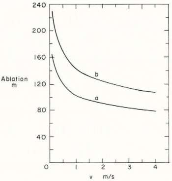
Fig. 6. Total average amount of ablation on a submerged face of an iceberg as a function of the relative towing velocity v which is here assumed to be constant over the complete transit. Curves (a) and (b) represent the great-circle routes for the Amery–Australia and the Ross–Atacama transits respectively. The ocean is assumed to be motionless and the initial lateral dimension of the iceberg is taken as 1 000 m.

Fig. 7. Total average amount of ablation for the Amery–Australia traverse as a function of the initial lateral dimensions of the iceberg face x 1. It is assumed that v = 0.5 m/s and that the ocean is motionless.
Trajectories, Towing Times, and Ice Delivered
The previous discussion of melting along great-circle routes is, of course, not realistic. Although the great-circle distances for the Amery–Australia and the Ross–Atacama transits are the shortest, they are not the easiest because of the winds and currents along the routes. In addition as the iceberg moves north, the decrease in size caused by melting will permit higher towing velocities. To estimate properly towing times and the amount of ice that can be delivered, it is necessary to consider all these factors simultaneously. The basic steady-state equation which applies is
where F is the towing force, τ a the air stress, τ w the water stress (drag), C the Coriolis force, and G the gradient current force. This equation must be solved simultaneously with the melt equation (8) to find the optimum towing path and towing force for each iceberg of a given size and shape. In order to solve this difficult system of equations, several assumptions are made. The first of these is that the towing force remains constant. This is a reasonable approximation as long as the velocity change along the route is small, as will be seen to be the case. Second, it is assumed that it is meaningful to use the mean wind velocity and gradient current fields of the Antarctic seas given by the U.S. Weather Bureau Antarctic Summary and the Atlas Antarktiki (i.e. the equations are solved only for seasonal mean fields and not for short-term phenomena such as individual cyclones).
Wind velocity vectors were plotted for a wide variety of possible routes between given collection and delivery sites. It was then assumed that along the route the wind stress plus the towing force was equal to the drag or water stress. As was discussed earlier, both the τ a and the τ w terms have a form drag as well as a skin drag term. If the iceberg has dimensions of x w (width), x 1 (length), x f (freeboard), x d (draft) and x t = x f + x d (thickness), it is assumed that the form drag component of τ a and τ w will act on the smallest face of the iceberg, that is on x w x f and x a x w respectively since x w ⩽ x 1. The skin drag term of τ a and τ w acts both on lateral faces and on the top and bottom faces (skin air stress acts on x w x 1+2x f x 1and skin water stress acts on x w x 1+2x d x 1). Considering Equations (1) and (2) and assuming that a Prandtl logarithmic boundary layer exists on the top and lateral freeboard sides of the iceberg, we can write the equation τ w = F + τ a as follows

where ρ a and ρ w are the air and water densities, C Da and C Dw are the form drag coefficients for air and water, v is the magnitude of the iceberg velocity relative to that of the surface water, v a is the wind velocity, z is the height of the wind-velocity measurement, z 0 is the surface roughness, κ 0 is the von Kármán’s constant, and v is the dynamic eddy viscosity. Equation (10) must be solved simultaneously with Equation (8) to estimate melting and to calculate v along each route. At each point the gradient current is known, and the velocity of the iceberg relative to the Earth’s coordinate system, which we will refer to as the transit velocity v t, is given by the vector sum
where G c, is the gradient current vector. The Coriolis force at each point along each route is then given by
where ω is the angular velocity of the Earth, ϕ is the latitude, and ρ i is the density of the ice.
A field of v t was computed for each iceberg choice and route area by graphically including the Coriolis and gradient current forces. At an array of points adjacent to and along possible optimum towing routes, the direction of the towing force F was varied so that the vector sum of Equation (9) provided the greatest v t in the desired direction. Then the optimum transit route was chosen by trying successive solutions to a string of v t solutions such that

Although this is a difficult operation, the fact that the gradient current and wind vectors are almost colinear and do not vary greatly along the optimum towing paths greatly simplifies the process. The reason we performed this combined numerical and graphical solution to Equations (8) through (13), rather than attempt a full numerical solution, is that such a solution would have been both laborious and costly. It also would not have resulted in a significantly improved analysis considering the limited data available on both the winds and currents of the Southern Ocean and on the change in the form drag coefficient of the iceberg as towing and melting progresses. However, as better data become available, we plan to make a time-dependent study of the full vector equations. Indeed, we feel that such calculations are essential before field towing tests are initiated.
Equations (8) through (13) were then solved for a variety of iceberg sizes assuming a constant initial ice thickness of 250 m and a length: width ratio of 4. The optimum paths for the Amery–Australia and the Ross–Atacama routes lie in two well-defined envelopes shown in Figure 8. Representative distances are 6 940 km and 8 990 km respectively as compared with distances of 5 550 km and 7 770 km by the great-circle routes. The following values were used for the constant terms: C Dw = C Da = 0.6, ρ w = 1 030 kg/m3, ρ i = 850 kg/m3, z = 10 m, z 0 = 2.0 × 10⁻⁴ m, v = 1.826 × 10⁻⁶ m2/s and κ 0 = 0.4. In Figure 9, the variations in the volume of the iceberg, the transit velocity along the route and the ice thickness are plotted against the distance along the towing route for the Amery–Australia and the Ross–Atacama transits for a towing force of 18.4 × 10⁶ N. The values shown are for an iceberg whose initial dimensions were 2 800 m × 11 200 m × 250 m. As expected, the melting during transit causes a significant loss of ice (the final dimensions of the icebergs are 2 703 m × 11 072 m × 202 m and 2 675 m × 11 034 m × 187 m respectively). This melting, in turn, causes a reduction in the drag along the route, and an associated general increase in the towing velocity. The fact that the highest transit velocities do not occur at the end of the towing period is caused by high winds and gradient currents during the middle portion of the transit. Figure 10 shows the volume of ice delivered as a function of the initial iceberg width. The widths of the “ice delivered” curves show the variation in the ice delivered as the towing force changes from 1.3 × 10⁶ N to 18.4 × 10⁶ N. Also, as anticipated earlier, major changes in the towing capability of the tug make only minor changes in the amount of ice delivered. In Figure 11, the amount of ice delivered is expressed as a percentage of the initial volume at time of pick-up. Again, as anticipated by Figures 5 and 7, the importance of melting in reducing the volume of icebergs whose initial dimensions are less than 1 km is clearly shown.

Fig. 8. Optimum towing paths between the Amery Ice Shelf and Australia and the Ross Ice Shelf and the Atacama Desert.

Fig. 9. Changes in iceberg volume V, iceberg thickness x t and transit velocity v t as a function of distance travelled along the towing routes between the Amery Ice Shelf and Australia and the Ross Ice Shelf and the Atacama Desert. The initial iceberg dimensions are 2 800 m × 11 200 m × 250 m and the towing force is 18.4 × 10⁶ N.

Fig. 10. Volume of ice delivered as a function of initial iceberg width. The initial thickness is assumed to be 250 m and the initial length is four times the width. Envelope width denotes variations caused by different towing forces.

Fig. 11. Amount of ice delivered expressed as a percentage of the initial volume of ice at the time of pick-up versus the initial iceberg width. The initial length and thickness are taken to be four times the width and 250 m respectively. Envelope width denotes variations caused by different towing forces.
Although changes in the towing force do not make large differences in the volume of ice delivered, they do make large changes in the transit times and, therefore, in the delivery rates. Figures 12 and 13 show transit times as a function of initial iceberg width and towing force while Figure 14 shows the ice delivery rate (assuming continuous ship operation) measured in cubic kilometers per year as a function of the same two parameters. The reader will note that for the case of the smallest towing force (1.3 × 10⁶ N), both Figures 12 and 13 show that for initial iceberg widths above a critical width, 2.7 km for the Amery–Australia route and 1.7 km for the Ross–Atacama route, the transit times decrease for icebergs of increasing width. This is so because the form and skin air stresses acting on the iceberg increase as its width increases and when a certain critical width is reached relative to the towing force, F is no longer the predominant driving force as it is for small iceberg widths.

Fig. 12. Transit times for the Amery–Australia tow as a function of initial iceberg width and towing force for initial lengths of four times the width and initial thicknesses of 250 m.

Fig. 13. Transit times for the Ross–Atacama Desert tow as a function of initial iceberg width and towing force for initial lengths of four times the width and initial thicknesses of 250 m.

Fig. 14. Ice delivery rate as a function of initial iceberg width and towing force for initial lengths of four times the width and initial thicknesses of 250 m.
As expected, the delivery rate is appreciably higher on the Australian traverse than on the Atacama traverse. In both cases, however, the volume of ice that can be delivered each year is impressively large, in the tens of cubic kilometers. A large delivery rate does not, however, necessarily mean an economically interesting delivery rate. The final question that remains is whether or not such a towing operation is economically attractive.
In concluding this section, we would like to stress that we feel that our analysis of the towing problem is a very crude first approximation at a quantitative analysis of a geophysically difficult problem. In particular, it can be argued that the use of seasonally averaged maps of Antarctic winds and ocean surface currents, produced as they were from an admitted scarcity of data, will give results that would not hold for the actual case of iceberg drift under the influence of short time-scale events; i.e. when a passing cyclone causes icebergs to drift in loops and other irregular trajectories. This may be. However, since no wind or current data exist for other than the seasonal case, an initial analysis of iceberg towing can only be made in some framework such as we have suggested. In addition, since such major parameters as suitable drag coefficients are at present only informed guesses, it would seem reasonable to acquire greatly improved data on these parameters before attempting a detailed analysis of icebergtowing on a small time scale. Later in this paper more will be said about studies necessary to improve the towing calculations.
Economics
An adequate economic analysis of “icebergs as a fresh-water source” is difficult. It clearly depends on a large number of factors, many of which are peculiar to the specific site that is selected. An appreciation of the complexity of the problem can be gained by studying recent planning documents that discuss the feasibility of large scale desalination projects in various parts of the world (United Nations, 1964; Oak Ridge National Laboratory, 1968). Such a study is clearly beyond our capability. However, in the present report we wish to appraise only the economics of transporting icebergs to suitable coastal sites. If this portion of the total operation can be shown to be very inexpensive relative to the price the processed water would command, then this should serve as an incentive for further research on the overall problem of the development of agro-industrial complexes that utilize iceberg water. It should also be noted that because we will discuss the economics of iceberg towing as if it were a wholly privately financed venture, it does not mean that we feel that such a case is likely. Indeed the large amounts of land required by such a project would necessitate, at least, partial governmental participation. However, if the venture can be shown to be attractive as a private venture, it certainly should be attractive as a governmental venture.
Our problem, therefore, amounts to estimating the operating costs of tugs that are appreciably larger than tugs currently in existence. Let us consider first the operating cost of the 1.56 × 10⁸ W super tug that was discussed earlier (towing force 18.4 × 10⁶ N). This cost consists of construction, crew and administration, maintenance, fuel, and interest. Fortunately, a design exercise has been completed on an Arctic icebreaking ship with identical powering (Reference Voelker and SlocumVoelker, 1972). Estimates of the construction cost (foreign) of a tug with a similar power are $60 million. To estimate the average cost of capitalization, we will assume a 25-year life for the tug (one twenty-fifth of $60 million or $2.4 million). To this we must add interest on the unpaid balance (using the approximate cost during the middle year of operation) which amounts to $3 million if a 10% interest rate is assumed. Therefore our total capitalization cost is roughly $5.4 million/year or $14 795/day. Here we neglect any financial advantage that might result from a favorable tax structure for the venture. In addition we have a crew cost of $2.1 million/year ($5 750/day) assuming a crew of 60 and a total salary-plus-administrative cost of $35 thousand/crewman-year. Maintenance and repair would come to an additional $1 million/year ($2 740/day).
The principal operational expense would, of course, be fuel. If the propulsion plant is gas turbine, the fuel consumption can be estimated from the relation (0.24 kg of diesel/kWh) giving roughly 900 000 kg of fuel/day. Assuming a cost of $2.80/barrel (114 kg), we have an estimated fuel cost of $22 100/day operating at full power. Therefore, the daily cost of the tug during towing is $45 400. During the return part of the cruise, when the tug is not towing, a great reduction in power is possible. For instance if 2.6 × 10⁷ W are utilized in open-sea cruising, this corresponds to a daily fuel cost of $3 680 and an operating cost of $27 000. At a cruising speed of 18 knots (800 km/d) the return trip to the Antarctic from Australia would take 7d and from the Atacama, 10 d. The daily cost while the tug is in port or in a shipyard is correspondingly $23 300. If we assume 10% port and shipyard time, we obtain a total yearly cost for tug operation of $15.5 million. There is no appreciable change in this cost between the Amery–Australia and the Ross–Atacama transits.
A similar exercise was completed for both a 4.5 × 10⁷ W tug with an estimated construction cost of $ 17 million and the tug Oceanic which has 1.1 × 10⁷ W and a construction cost of $2.5 million ( New York Times, 1969). The resulting total costs were $5.6 million and $1.8 million/year respectively. These figures were then used to develop a crude curve relating total operational cost per year to the power of the tug.
Now we know from Figure 14 the delivery rate in terms of cubic kilometers of ice per year for four different sized tugs. These estimates were first reduced by 10% to allow for shipyard time. Then the volume of ice was converted to an equivalent volume of water by multiplying by 0.85. Next curves were plotted for a variety of initial iceberg widths giving the delivery cost of ice, expressed in terms of the equivalent amount of water, versus the towing force (Figs. 15 and 16). In looking at these figures, it should be remembered that a towing force of 1.3 × 10⁶ N corresponds to the Oceanic, 6 × 10⁶ N to a tug with powering similar to the U.S. Coast Guard Icebreaker Polar Star which is currently under construction, and 18.4 × 10⁶ N to a 1.56 × 10⁸ W super-tug.

Fig. 15. Delivery cost per cubic meter of water delivered as ice to Western Australia expressed as a function of towing force and initial iceberg width, initial length four times the initial width. The dashed cross-curves give the sizes of icebergs that can be towed at the indicated steady-state velocities as a function of the towing force if a form drag coefficient of 0.9 is assumed.
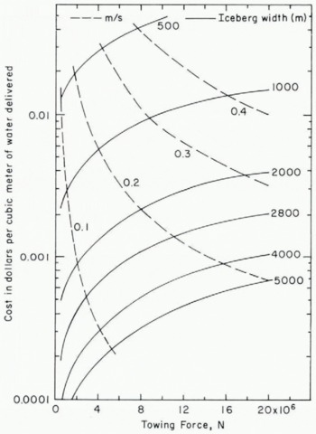
Fig. 16. Delivery cost per cubic meter of water delivered as ice to the Atacama Desert expressed as a function of towing force and initial iceberg width, initial length four times the initial width. The dashed cross-curves give the sizes of icebergs that can be towed at the indicated steady-state velocities as a function of the towing force if a form drag coefficient of 0.9 is assumed.
Figures 15 and 16 tell us a great deal about the economics of iceberg transportation. At first glance, delivery costs appear amazingly low. Costs in the range of a fraction of a mill (1 mill = $0.001) per cubic meter of water are certainly competitive by any standard even if delivered in the form of ice. However one must realize that the whole range of values shown in Figures 15 and 16 is not available. If the towing force is so small that only extremely low speeds can be achieved, the tug will not be able to control the iceberg. This restriction is indicated in the figures by the dashed cross-curves which give the sizes of icebergs that can be towed at the specified steady-state velocities as a function of the towing force. These cross-curves are based on the calculations that are summarized in Figure 4a (i.e., a form drag coefficient of o.g and an iceberg length: width ratio of 4 are assumed). Therefore only prices “above” the appropriate minimum control-speed cross-curves can be realized. Clearly to minimize our delivery costs we should use as large a tug as possible. This tug should then tow the largest possible iceberg at the lowest velocity that still allows it to maintain control over the tow. We do not know what the lowest possible control velocity is, but its value for the large tows considered here is clearly critical. For instance, if we have a super-tug capable of exerting a towing force of 18.4 × 10⁶ N, the delivery costs are 7 mills/m3 of water if the control velocity is 0.4 m/s and on the order of 0.04 mills/m3 if the velocity is 0.1 m/s. In the following discussion we will consider 0.25 m/s as the lowest permissible towing velocity. Therefore, using a super-tug, costs would be 1.3 and 1.9 mills/m3 for water delivered as ice to Australia and the Atacama Desert, respectively.
We could now use the current estimated production costs of large desalination plants as a measure of the price of water ($0.19/m3). This would allow us to spend the difference between the selling price and the delivery cost on processing the ice. Because our delivery costs are less than 2 mills/m3, we could afford to spend up to $0.18/m3 on processing. Attractive as these figures are, they clearly are not realistic. Although water prices under certain situations may clearly equal or exceed $0.19/m3 (prices in excess of $2.50/m3 occur in a number of areas served by desalination plants; United Nations, 1964), such water is usually utilized for municipal water supply or special purpose projects. From our previous analysis, it appears that iceberg towing as a water supply mechanism becomes most attractive when very large volumes of ice are involved. That is not to say that iceberg water could not be used for municipal water supply. It certainly could, but probably only as a small part of an operation designed to supply much larger volumes of water to an irrigation or a large industrial complex. We therefore believe that the economic appraisal of iceberg water should be based on the price of irrigation water.
A realistic price for irrigation water is, in itself, difficult to establish. This is true even in areas where the utilization of irrigation water is well developed (Reference Clawson, Clawson, Landsberg and AlexanderClawson and others, 1969, Krous and others, 1969). We could use the U.S. Federal price goal for irrigation water produced by desalination ($0.03/m3). This is roughly the production cost for surface water, and values in this range have been used recently in planning studies (Oak Ridge, 1968). However, current studies suggest that even this value is high and that a value of 8 mills/m3 is a much more realistic planning standard (Reference Clawson, Clawson, Landsberg and AlexanderClawson and others, 1969). This is in the range of the cost of producing ground water from a large, high-quality well ( Water Newsletter, 1969). In short, if water can be delivered at a cost of a few mills per m3, the development of large irrigation projects would indeed appear to be highly attractive. As has been shown, this is the case for both Western Australia and the Atacama Desert region. In these two locales, one can use, respectively, 6 and 4 times the delivery cost of the ice at the coast to moor the iceberg, melt the ice, and pump the melt water inland.
Our discussion of the towing problem is in most cases a “worst case” analysis. In particular, we have calculated travel times and en-route melting from the edge of the Amery and Ross Ice Shelves. In fact, the nearest suitable icebergs, as located by satellite surveillance would be utilized with significant savings in delivery costs over those estimated in this paper. Available information on iceberg sightings (Reference NazarovNazarov, 1962) suggests that cost savings of 25% might easily be realized. The data required to perform an analysis of this aspect of the towing problem will soon be available based on studies of the imagery from the ERTS and NIMBUSE satellites. It is also to be expected that by the time of pick-up, melting would have caused an appreciable reduction in the form drag coefficient of those “weathered” icebergs from the value of 0.9 assumed for initial towing in the present paper. These considerations suggest to us that the costs of iceberg towing to Australia and the Atacama Desert are probably lower than the values suggested here.
Problems Related to Iceberg Transport
It would be easy to present a long “shopping list” here. We are certain that each reader feels that at least one of his pet problems has been neglected or even ignored. In this discussion we will only mention problems that we consider to be major.
First, additional information should be collected on iceberg distribution and geometry. As discussed earlier, by 1973 satellite imagery having direct bearing on this problem should be available. The recently obtained ERTS imagery of ice in Hudson Bay and Beaufort Sea has a resolution better than 100 m. Complete coverage of the Southern Ocean should soon be available every 18 d (weather and sunlight permitting). Field observations should also be made on the condition of the icebergs that are located at the more northerly latitudes. When this work is completed, it should be possible to base a towing analysis on the distance from the most probable pick-up location to the delivery site.
The towing analysis itself could be greatly improved. First, it would be very useful to have better form drag coefficients for Antarctic icebergs. These values are important because they determine the largest iceberg that a given tug can tow at a controllable speed at pick-up. As shown, the size of this iceberg fixes much of the resulting economics. If these drag coefficients cannot be determined by direct towing because of cost, at least studies could be made with model icebergs. Because of the highly irregular shapes of most “Greenland” icebergs, we doubt that data currently being collected on them will prove to be readily applicable to the Antarctic towing problem. Secondly, a more realistic appraisal of in-transit melting should be made. In the present treatment we simply calculated an average melting rate and assumed parallel recession of the walls. This is, of course, incorrect. The most rapid melting occurs at the front of a face and gradually decreases toward the rear. The result of this uneven melting is a rapid streamlining of the iceberg as it is towed. Not only should the change in shape be calculated, experimental observations should also be made so that these changes can be used to estimate changes in the form drag coefficient as melting progresses. In addition a check should be made of the applicability of Equation (4). Recent studies of the melting of the lower surface of river ice (Reference Ashton, Landis and HordemannAshton, 1972, unpublished) have shown that the ice surface does not remain smooth but develops a series of ripples. The presence of the rippled ice surface appears to be associated with an increase in both the heat transfer rate and in the flat-plate drag. If a similar phenomenon occurs during the melting of icebergs, it definitely should be taken into account. Methods have been suggested (personal communication from J. Hult) that would minimize in-transit melting by utilizing a plastic shield to maintain a layer of cold water at the ice surface. This certainly is conceptually possible. However, considering the size of the proposed tows, such a shield, even if utilized only on the forward end of the iceberg, would be both costly and difficult to emplace. The shield would probably be even more difficult to keep in place while towing. At least the possibility of such a scheme should be explored, particularly if iceberg tows to delivery sites nearer to or across the equator are contemplated.
Once the information discussed above is available, a revised towing calculation should be performed that takes these new factors into account. This improved calculation should also include the acceleration of the iceberg at the start of the tow and the deceleration at the end. It would, as mentioned earlier, be nice to have sufficiently detailed information to permit a time-dependent towing analysis that includes the effects of short-term meteorological and oceanographic events. It is, however, doubtful that such detailed information will be available in the near future. An analysis of existing meteorological information should, nevertheless, be adequate to permit a crude estimate of the towing time that would be lost as the result of high seas. This lost time will, undoubtedly, be related to the size of both the tug and the tow. If all the above information can be combined with a correction factor that estimates the amount of ice that will probably be lost during a tow by the calving of fragments from the main iceberg, we would guess that the result would serve as quite an adequate base for an economic analysis of the towing aspect of an iceberg delivery system.
Processing
The problem of processing the iceberg once it has been delivered at the coast is clearly one in which a great deal of ingenuity could be exercised. This is primarily an engineering problem that is outside our area of expertise. We will, however, discuss the general problems that can be anticipated. Because of the deep draft of most icebergs at their time of arrival, many operations will probably have to take place at some distance from the coast unless a suitable deep harbor is available. Once the iceberg is moored, a scheme suggested by Isaacs (Reference BurtBurt, 1956[b]) would seem to be a very attractive way to separate the melt water. In this approach the iceberg is surrounded by a floating fence-like baffle that extends some distance below sea-level. The fresh melt water would form a stable layer on top of the sea-water inside the baffle. From there it could be pumped to a coastal station. It is also possible that some method of quarrying the ice and moving a slurry to the coast could be useful although this would require the processing of ice on an unprecedented scale.
It should also be remembered that the total volume of water produced by a given iceberg is appreciably greater than the volume of water produced by the melted ice. During the melting process there will be a continual condensation of water on the cold iceberg surface as the result of the contact cooling of the warm, humid air at the delivery site. If an iceberg is allowed to melt slowly, the amount of water that would be produced by this process could be very significant. This would be particularly true for the Atacama Desert docking site. Experimental studies have been undertaken recently at the Universidad del Norte de Antofagasta (United Nations, 1964, p. 104–05) to develop methods for collecting fresh water from the dense fogs that are formed every night by the cool Humboldt Current.
Irrigation water can contain an appreciable impurity concentration. The melted ice is, however, extremely pure, containing usually less than 10 p.p.m. impurities (Reference GowGow, 1968). The melt water can, therefore, be mixed with sea-water to bring the impurity concentration up to the allowable level, thereby increasing the volume of water that can be delivered. Irrigation water containing 400 p.p.m. impurities is considered to be excellent for all crops, while 900 p.p.m. water can be tolerated by most crops (comparable to the salinity of the water in the lower reaches of the Colorado River). A few crops such as cotton can be raised even with impurity levels as high as 1 500 p.p.m. (Reference Krous, Krous, Wagner and FerneliusKrous and others, 1960). To achieve these concentration levels 1.1, 2.6 and 4.5% (by volume) sea-water can be added to the melt water. There will, of course, also be water losses during the melting process. These are difficult to estimate because they depend on the details of how the iceberg is handled, a matter which is at present not resolved. Therefore, we will neglect the water additions and assume that they will roughly balance the water losses.
One other aspect of the processing of the ice should be remembered. Regardless of the engineering details, the iceberg during processing serves as an extremely large heat sink. The iceberg towing scheme could, therefore, be most favorably coupled with a major power generation project. The thermal pollution associated with the power generation would then become a valuable asset in the conversion of ice to water. Such a combined major nuclear energy center with associated industrial and agro-industrial complexes has been discussed by the Oak Ridge National Laboratory (1968) in conjunction with the desalination of sea-water. Based on the present study, it would appear that the development of such a complex in association with an iceberg transportation scheme could have great economic as well as environmental advantages.
At the present we do not see any major engineering obstacles to processing icebergs that could not be overcome with existing technology. We would guess that it would be a rare engineer who would not consider the design of an iceberg processing facility, within the economic constraints that we have outlined, to be an interesting problem indeed.
The environmental effects of an iceberg towing program should also be investigated. Although the in-transit effects would be expected to be minimal, the icebergs would definitely cause localized thermal pollution with an associated drop in the sea temperature near the delivery site. In addition there would be a decrease in the salinity of the sea-water as the result of the mixing of “escaped” fresh water during the melting process. There is also the possibility of changes in the local climate in the vicinity of the moored icebergs; for instance the increased occurrence of fog and rain. It is difficult to quantitatively analyze these changes. However, we do not believe that they would prove to be major problems. The undesirable environmental effects upon the marine biota associated with a drop in the sea or air temperature below normal values would probably be less than expected from a similar rise in temperatures above the normal. There would, however, undoubtedly be significant local changes in the marine life around the delivery site. If a near steady-state temperature and salinity are developed in the vicinity of the delivery site, a new ecosystem would develop that might be more biologically productive.
Conclusion
We would like to stress that we, in no way, feel that the present study is an adequate look at the “iceberg” problem. It is merely a first approximation at a quantitative assessment of the availability and transportation aspects of the problem. Unless our analysis is grossly in error, the results of this portion of the study are very exciting. The possibility of delivering ice to coastal sites in Australia and western South America for costs of a few mills per cubic meter is certainly sufficient motivation to explore the problem in considerably more detail. We have also tried to outline where research is needed and what aspects of the problem should be considered next. In addition, we have discussed some approaches that have been suggested for processing the iceberg once it has reached the coastal site. Although there are a number of major engineering problems that must be overcome, it is our impression that they are within the reach of existing technology. The problems are, however, sufficiently varied (oceanography, meteorology, glaciology, fluid mechanics, naval architecture, marine biology, agriculture, economics) that an adequate appraisal of the problem is beyond the capability of a few individuals or even one major research group. We hope that our efforts on this subject will interest other specialists in giving the problem the detailed analysis that it appears to merit.
If our preliminary appraisal is approximately correct, the development of an operational iceberg transportation scheme offers the possibility of efficiently utilizing some arid coastal areas in the Southern Hemisphere for large-scale agriculture and perhaps for large agro-industrial complexes. The amount of land that could be placed under irrigation is very large. For instance if only one super-tug (18.4 × 10⁶ N) delivers ice to Western Australia, the steady-state amount of melted water (≈ 12 × 109 m3 of water per year) would irrigate over 16 × 103 km2 of land. This corresponds to a square field 126 km on a side. This assumes that 0.76 m3 of water is required per m2 of land (Reference ToddTodd, 1970). The amount of water (12 × 109 m3) is roughly four times the amount provided by the Snowy Mountains Project (Reference OvermanOverman, 1969, p. 82) and can be increased to virtually any larger amount by simply constructing more tugs.
The best aspect of the scheme discussed in the present paper is that its principal resource, the icebergs, are currently being completely wasted as regards man’s needs. They calve from the Antarctic ice shelves and slowly drift in the Southern Ocean until they eventually melt. The towing proposal simply utilizes small amounts of power to break selected icebergs through the “barrier” of the Antarctic convergence and deliver them to points where large volumes of fresh water are needed. There, the water, after being utilized for irrigation, eventually returns to the sea. The end result is the same, only the path is different. We would guess that the potential rewards to man of the more tortuous path will prove to be well worth the additional energy expenditure, not only in terms of increased food production but as a more ecologically sound way of alleviating water scarcity than the more frequently mentioned sea-water desalination techniques with their resultant great positive thermal pollution. Indeed, iceberg towing in temperate and sub-tropical waters may help to counter the increasing warming of surface waters due to man’s energy production.
Acknowledgements
The authors would like to thank Dr H. Bader for interesting them in this general problem. A. Rassmussen, U.S.G.S., made the towing calculations. Numerous other people provided technical and historical information. Among these should be mentioned G. Ashton, A. Assur, C. Clark, A. Cook, R. Edwards, L. Giordano, J. Hult, J. Isaacs, C. I. Jackson, P. Kimon, A. Kohn, R. D. Parkhurst, H. Richardson, B. Roberts, T. Savill, Jr., R. Schwartzlose, R. Voelker and Y. C. Yen. A. Johnson and S. Bowen helped with the editing of the final manuscript.


