


Introduction
The worldwide geothermal power capacity amounts to 15.4 gigawatts (GW) as of 31 December 2019 (Richter, Reference Richter2019). In the Netherlands, 24 geothermal doublets have been realized as of 1 January 2019 (Mijnlieff, Reference Mijnlieff2020). The geothermal reservoirs in the Netherlands are the same as the ones targeted for oil and gas. With a geothermal gradient of approximately 31°C/km and an average surface temperature of 10°C (Bonte et al., Reference Bonté, van Wees and Verweij2012), the subsurface between 1.5 and 3.0 km depth is considered suitable for geothermal exploitation with temperatures ranging between 60 and 100°C. The majority of the installed doublets in the Netherlands target porous and permeable sandstone reservoirs including the Rotliegend, the Lower Germanic Triassic and the Upper Jurassic/Lower Cretaceous primarily in the West Netherlands Basin (Bekesi et al., Reference Bekesi, Struijk, Bonte, Veldkamp, Limberger, Fokker, Vrijlandt and Wees2020).
In this study, the Slochteren formation (part of the Permian deposits of the Upper Rotliegend group) was selected as the primary sedimentary geothermal reservoir of interest, because it is widely used for geothermal energy production and it extends throughout the Netherlands. Additionally, the Delft sandstone member (Lower Cretaceous), as a local porous sedimentary reservoir, and the Dinantian limestone (Carboniferous), as deep fracture/karst dominated geothermal reservoir, were investigated in this study. The latter formation could potentially serve as a target for a future enhanced geothermal system (EGS). Currently, no such projects are in operation in the Netherlands. However, the large potential of these systems, ongoing research (e.g. Moore et al., Reference Moore, McLennan, Allis, Pankow, Simmons, Podgorney and Rickard2019; Huenges et al., Reference Huenges, Ellis, Welter, Westaway, Min, Genter, Brehme, Hofmann, Meier, Wassing and Marti2020) and recent breakthroughs in EGS technology (Norbeck et al., Reference Norbeck, Latimer, Gradl, Agarwal, Dadi, Eddy, Fercho, Lang, McConville, Titov, Voller and Woitt2023) could lead to a future use of the Dinantian limestone.
No major induced seismic events have yet been recorded in any of the Dutch geothermal sites in hot sedimentary aquifers Buijze (Reference Buijze2020). The only reported seismicity related to geothermal operations in the Netherlands are events with a maximum magnitude of 1.7 at the Californië site, which accesses a deep fault zone in the Dinantian limestones (Vörös & Baisch, Reference Vörös and Baisch2022). Nevertheless, the possibility of induced seismicity inhibits an even faster development of the geothermal sector. Induced seismicity refers to seismic events caused by human interventions (Foulger et al., Reference Foulger, Wilson, Gluyas, Julian and Davies2018). These seismic events are a direct result of changes of the stress state in the subsurface causing rapid slip along a pre-existing region of weakness (faults/fractures). If the in situ stresses are close to a critical state with respect to the orientation of major faults, even a relatively small change in stresses may lead to seismic (or aseismic) failure of a fault.
In this study, coupled thermo-hydro-mechanical (THM) simulations were carried out to analyse the impact of various geological and operational parameters on the failure potential of a pre-existing fault in typical Dutch geothermal reservoirs. The THM computations were performed with the multi-physics, multi-component open source simulator GOLEM (Jacquey & Cacace, Reference Jacquey and Cacace2017; Cacace & Jacquey, Reference Cacace and Jacquey2017). The relative influence of key geological and operational parameters on the slip tendency of pre-existing faults was investigated with a sensitivity analysis in a synthetic geothermal reservoir model of the Slochteren sandstone formation, the Delft sandstone formation and the Dinantian limestone formation in the Netherlands. Among those parameters, a focus of our study is on the effect of re-injection temperature and related stress changes on fault stability, which likely plays a major, yet often ignored, role in injection-induced seismicity (Ghassemi et al., Reference Ghassemi, Tarasovs and Cheng2007; De Simone et al., Reference De Simone, Vilarrasa, Carrera, Alcolea and Meier2013; Wassing et al., Reference Wassing, Candela, Osinga, Peters, Buijze, Fokker and Van Wees2021; Kivi et al., Reference Kivi, Pujades, Rutqvist and Vilarrasa2022).
Numerical approach
The simulation code GOLEM uses a Galerkin Finite Element technique to solve for the parallel implicit non-linear coupled initial-boundary value problem. Balance equations of fluid and solid mass, heat and momentum serve as the base for the numerical formulations of the governing equations for fluid-flow, heat transport and elastic deformation (Cacace and & Jacquey, Reference Cacace and Jacquey2017).
Darcy’s law correlates the Darcy’s flow rate per unit of surface area or Darcy velocity ( q D ) with porosity (n), fluid velocity ( v f ) and solid velocity ( v s ) and by expansion with the reservoir permeability ( k ), fluid viscosity (μ f ), pore-fluid pressure (p f ), fluid density (ρ f ) and acceleration due to gravity ( g ).
 $${{\boldsymbol{q}}_{\boldsymbol{D}}} = n\left( {{{\boldsymbol{v}}_{\boldsymbol{f}}} - {{\boldsymbol{v}}_{\boldsymbol{s}}}} \right) = - {{\boldsymbol{k}} \over {{\mu _f}}}.\left( {\nabla {p_f} - {\rho _f}{\boldsymbol{g}}} \right)$$
The mechanical governing equation is given by
 $$\nabla .\left( {\sigma ^\prime - \alpha {\mkern 1mu} {p_f}{\boldsymbol{I}}} \right) + {\rho _b}g = 0$$
where σ′ denotes the effective stress, α denotes the Biot’s coefficient of the reservoir rock, ρ b denotes the bulk density of the rock-fluid system and I is an identity matrix. The effective stress is given by Equation (3).
 $$\sigma ^\prime = \sigma + \alpha {\mkern 1mu} {p_f}{\boldsymbol{I}}$$
The change in the effective thermal stress for non-isothermal deformation is proportional to the drained thermal expansion coefficient (β d ), the material stiffness matrix ( C ) and the change in temperature (ΔT).
 $$\Delta {\sigma ^\prime }_T = {1 \over 3}{\boldsymbol{C}}{\beta _d}\Delta T{\boldsymbol{I}}$$
The equation of internal energy conservation consists of the temporal, convective and conductive parts.
 $${\left( {\rho c} \right)_b}{{\partial T} \over {\partial t}} + {(\rho c)_f}{q_D}\nabla T - \nabla \ .\ ({\lambda _b}{\mkern 1mu} \nabla T) = 0$$
where (ρc) b denotes the bulk specific heat, (ρc) f is the fluid specific heat and λ b denotes bulk thermal conductivity.
The problem variables are pore fluid pressure, temperature and solid displacement, which results in a system of non-linear coupled equations. A detailed derivation of the formulations is described in Cacace & Jacquey (Reference Cacace and Jacquey2017). A weighted residual method is then applied to the system of equations to obtain the weak forms of these governing equations. The weak forms of the governing equations are solved either by Newton–Raphson or Free Jacobian Inexact Newton Krylow schemes (Cacace & Jacquey, Reference Cacace and Jacquey2017).
The fault failure potential is estimated in terms of a parameter referred to as ‘slip tendency’ ( ${\rm {ST}}$
), which is defined as the ratio of the resolved shear stress (τ) and the effective normal stress (
${\rm {ST}}$
), which is defined as the ratio of the resolved shear stress (τ) and the effective normal stress ( ${\sigma _n ^\prime}$
= σ
n
− p
f
) on the fault plane (Morris et al., Reference Morris, Ferrill and Henderson1996; Ramsay & Lisle, Reference Ramsay and Lisle2000).
${\sigma _n ^\prime}$
= σ
n
− p
f
) on the fault plane (Morris et al., Reference Morris, Ferrill and Henderson1996; Ramsay & Lisle, Reference Ramsay and Lisle2000).
 $${\rm{ST}} = {\tau \over {\sigma _n ^\prime}}$$
The Mohr–Coulomb criterion is used to determine the failure of a fault plane. It states that slip occurs when the shear stress along the fault plane exceeds the static shear strength of the fault, which is given in terms of the fault friction coefficient (μ s ) and cohesion (S o ) as follows:
 $$\tau \ge {S_o} + {\mu _s}\,.\,\sigma _n ^\prime$$
For a cohesionless fault (S 0 = 0) slip occurs when
 $${\rm{ST}} \ge {\mu _s}$$
In this study, the static friction coefficient of the fault was taken as 0.6. A slip tendency value higher than 0.6 was therefore considered as an indication of fault failure.
We note that the slip tendency only gives a probability of (re)activation of the fault without providing information on whether the resulting fault is seismic or aseismic. Therefore, we performed an additional study, considering a rate and state formalism to describe the frictional behaviour of the fault, which we discuss in the supplementary text (Figures S1–S4). In addition, we refer to a companion study by Hutka et al. (Reference Hutka, Cacace, Hofmann, Zang, Wang and Ji2023) that uses the same model geometry and a different method introduced by Cacace et al. (Reference Cacace, Hofmann and Shapiro2021) to quantify the seismic response of the reservoir in the same scenarios presented in this study.
Model setups and scenarios
The THM simulation including slip tendency analysis with GOLEM has been validated at the Groß Schönebeck (GrSk) EGS site (Blöcher et al., Reference Blöcher, Cacace, Jacquey, Zang, Heidbach, Hofmann, Kluge and Zimmermann2018). This site accesses the Rotliegend formation below ∼3900 m.
The validated model was adapted to the condition in the different formations of interest in the Netherlands. All reservoir models were setup in a similar fashion. The coordinates of the model were aligned with the maximum (SHMax) and minimum horizontal stress directions (Shmin). This was done to avoid any shear stress accumulation along the edges of the model and the resulting distortion of the original model geometry. The finite element mesh was generated with the open source software MeshIt (Cacace & Blöcher, Reference Cacace and Blöcher2015). Mesh refinement was applied around the wellbores, along the fault and inside the reservoir unit. We used an adaptive time stepping, where the time step size increases with the number of nonlinear iterations at each time step with an upper bound of 1 year. A steady-state simulation run first to initialize the model in terms of pore pressure, temperature and relative displacements, consistent with the in situ reservoir conditions. This steady-state model was then used as starting model (initial conditions) for the subsequent transient runs covering a 30-year simulation period with cold water injection and production with the same flow rate.
Slochteren sandstone reservoir
The Slochteren sandstone model was simplified to three horizontal geological units: Zechstein (top seal unit), Slochteren (reservoir unit) and Limburg (bottom seal unit). All three units are intersected by a two-dimensional fault. The two wells are represented by one-dimensional line elements representing the open hole sections of the injection and production well, which intersect the entire reservoir unit. Figure 1 illustrates the top and side views of the Slochteren base case model. Figure 2 is a snapshot of the base case model mesh. Mechanical, hydraulic and thermal properties of the rock matrix of reservoir, top and bottom unit as well as fault properties can be found in Table 1. Fluid properties are summarized in Table 2. A summary of the model geometry and wellbore information is provided in Table 3. Detailed information on the boundary conditions are presented in Table 4.

Figure 1. Top view (top left) and side view (top right) for the Slochteren base case model (not to scale).

Figure 2. 3D view of the Slochteren base case mesh. Mesh refinement is applied around the injection and production wells and in the fault plane within the reservoir unit.
Table 1. Mechanical, thermal and hydraulic properties of geological units and the fault in the Slochteren sandstone base case model.

Table 2. Fluid properties of the Slocheren sandstone, Delft sandstone and Dinantian limestone models. The viscosity for the Slochteren and Dinantian models is a function of pressure and temperature derived from the data from the Groß Schönebeck Rotliegend reservoir fluid. In the Delft models, a pressure and temperature dependent viscosity function for pure water was used.

Table 3. Geometrical and wellbore properties of the Slochteren sandstone model (base case scenario).

Table 4. Slochteren sandstone, Delft sandstone and Dinantian limestone base case model boundary conditions.

Model geometry and boundary conditions
The top of the Slochteren reservoir varies between 1500 and 3000 m and its thickness varies between 100 and 250 m (Mijnlieff, Reference Mijnlieff2020). We chose the Middenmeer site with a top Slochteren depth of 2200 m and a thickness of 200 m as representative for the base case model (DESTRESS, 2021). The thickness of the overlying Zechstein group varies between <100 m (in marginal settings) and >1200 m (in the salt basin; TNO-GSN, 2021; Duin et al., Reference Duin, Doornenbal, Rijkers, Verbeek and Wong2006). The underlying Limburg group has typically a thickness of ∼600 m which can reach up to 1300 m (Dinoloket, 2021). To avoid any boundary effects, we used a 1000 m thickness for both top and bottom layer.
Fault patterns are relatively homogeneous across the whole onshore part of the Netherlands with a main fault trend varying between NW-SE and NNW-SSE and faults dipping in different directions (Duin et al., Reference Duin, Doornenbal, Rijkers, Verbeek and Wong2006; de Jager, Reference De Jager, Wong, Batjes and de Jager2007). We do not consider secondary fault systems that strike in different directions and we consider only a dip towards NE. Cross-sections in de Jager (Reference De Jager, Wong, Batjes and de Jager2007) show that most faults are sub-vertical. Thus, we assume a typical fault dip of 80° and tested variations in the dip angle between 60° and 85°.
The average temperature gradient in the Netherlands can be considered as 31°C/km with a surface temperature of 10°C and an uncertainty of ±10°C/km (Bonté et al., Reference Bonté, van Wees and Verweij2012). We therefore use 31°C/km + 10°C for the base case, 20°C/km + 10°C as minimum and 40°C/km + 10°C as maximum temperature gradient. Despite the possibility of local fluid overpressures (Verweij et al., Reference Verweij, Simmelink, Underschultz and Witmans2012), we assume an initial hydrostatic pore pressure gradient in our simulations. For this, we assume a minimum density of 1020 kg/m³, representative for seawater, and a maximum density of 1220 kg/m³, representative for a brine with salinity of ∼400 g/l, which is rarely exceeded in the Dutch Rotliegend (Veldkamp et al., Reference Veldkamp, Goldberg, Bressers and Wilschut2016). This corresponds to minimum and maximum pore pressure gradients of 10 and 12 MPa/km. For the base case scenario, we chose 11 MPa/km, representative for the GrSk geothermal site with 265 g/l salinity (Blöcher et al., Reference Blöcher, Zimmermann, Moeck, Brandt, Hassanzadegan and Magri2010).
We assume a normal faulting regime (SV > SHmax > Shmin) according to Guises et al. (Reference Guises, Embry and Barton2015). According to Verweij et al. (Reference Verweij, Simmelink, Underschultz and Witmans2012), the vertical stress gradient in the Netherlands is frequently below the standard gradient of ∼23 MPa/km (corresponding to ∼2300 kg/m³ bulk density). Van Eijs (Reference Van Eijs2015) shows vertical stress gradients increase with depth from ∼19 to 21 MPa/km at 1 km depth to 22–24 MPa/km (at 3 km depth). We therefore assume an average vertical stress gradient of 22 MPa/km for the base case scenario with a possible variation between 21 and 23 MPa/km. Note that these are average gradients over the entire depth range and only the corresponding effective horizontal stress values at a point located at the centre of the Slochteren formation are used for model calibration. The actual stress gradients in the individual layers depend on the elastic rock properties.
According to TNO (2015), the standard minimum horizontal stress gradient can be considered as 0.6 times the standard vertical gradient of 23 MPa/km (ΔShmin = 13.8 MPa/km). They find that the leak-off pressure, which is representative for the minimum horizontal stress, is rarely below this standard gradient and is also bound by the lithostatic stress gradient. Osinga & Buik (Reference Osinga and Buik2019) propose a Shmin gradient of 18 MPa/km for the deeper Dinantian formation. Guises et al. (Reference Guises, Embry and Barton2015) determined minimum horizontal stress gradients of 15.4–16.7 MPa/km for the Groningen gas field. We assume a minimum horizontal stress gradient of 14 MPa/km for the base case scenario with 13 MPa/km and 20 MPa/km as lower and upper bound, respectively.
Van Eijs (Reference Van Eijs2015) found relatively low differences between the minimum and maximum horizontal stress gradients in the Groningen gas field. Different methods yield a variation of the ratio SHmax/Shmin between 1.02 and 1.42. Osinga & Buik (2019) suggested SHmax as ∼5–20% higher than Shmin as a reference. Guises et al. (Reference Guises, Embry and Barton2015) determined maximum horizontal stress gradients of 17.3–18.2 MPa/km for the Groningen gas field. We assume a typical SHmax/Shmin ratio of 1.07 for the base case scenario (ΔSHmax = 1.07 * 14 MPa/km = 15 MPa/km), a lower bound for the SHmax gradient equal to the minimum horizontal stress gradient (14 MPa/km) and an upper bound of the SHmax gradient equal to 20 MPa (ΔSHmax = 1.42 * 14 MPa/km = 20 MPa/km). Note that SHmax has the largest uncertainty among all stress magnitudes.
According to Mechelse (Reference Mechelse2017), the pre- and post-salt stress directions are similar. The maximum horizontal stress direction in the Netherlands is typically NW-SE with values ranging between N130°E and N5°E (Heidbach et al. Reference Heidbach, Rajabi, Reiter and Ziegler2016). Guises et al. (Reference Guises, Embry and Barton2015) determined the maximum horizontal stress direction to be N160°E in the Groningen gas field. We assume N160°E for the base case scenario and a typical range between N150°E and N170°E for the sensitivity analysis. Note that stress directions may strongly vary locally since stress rotations can be expected near salt domes and fault zones, which we do not consider in our sensitivity analysis.
According to Mijnlieff (Reference Mijnlieff2020), the flow rate of geothermal wells accessing the Slochteren reservoir ranges from ∼40 to ∼100 l/s. We chose these values as lower and upper limits, respectively, and their median value of 70 l/s as representative for the base case scenario.
The well spacing (distance between production and injection well) is typically calculated as to avoid thermal breakthrough during the projected lifetime of the doublet. The well spacing of Dutch geothermal doublets is up to 1.5 km (Mijnlieff, Reference Mijnlieff2020). We therefore use 1.5 km as maximum well spacing. For the base case, we use a typical well spacing of 1 km and 0.5 km represents our lower bound for the sensitivity analysis.
Typically, a re-injection temperature of 25–35°C can be assumed for Dutch geothermal wells (Hurter & Schellschmidt, Reference Hurter and Schellschmidt2003; Wang et al., Reference Wang, Khait, Voskov, Saeid and Bruhn2019; Willems et al., Reference Willems, Nick, Weltje and Bruhn2017). We use a re-injection temperature of 30°C for the base case scenario. To evaluate the effect of the re-injection temperature, we use 20°C and 70°C as lower and upper bound.
We do not model the entire geothermal wellbores explicitly but approximate them as open 1D elements going through the entire reservoir layer. Therefore, we do not consider the wellbore diameter in our sensitivity analysis. However, we use a typical geothermal wellbore diameter of 8 ½” for the open hole section in all models.
We use a relatively short distance between wells and fault of 250 m for the base case scenario in order to easily see effects of different parameters on the temperature, pressure and stress distribution on the fault. For the sensitivity analysis, we vary this distance between 0 m (well intersects the fault) and 1000 m.
Rock matrix, fault and fluid properties
Geomechanical rock properties
Solid bulk modulus
The Slochteren reservoir sandstone primarily consists of quartz. According to Schmitt (Reference Schmitt and Schubert2015), the solid bulk modulus of Quartz is 37.8 GPa (α-Quartz) and 42.97 GPa (β-Quartz). We assume a solid bulk modulus of 40 GPa for the Rotliegend sandstone in the base case model. The Zechstein group may consist of calcite, dolomite, anhydrite and halite with a solid bulk modulus of 73.3 GPa, 94.9 GPa, 54.9 GPa and 24.9 GPa, respectively (Schmitt, Reference Schmitt and Schubert2015). We assume a solid bulk modulus of 30 GPa for the Zechstein formation in the base case model. Claystones, which we assume representative for the Carboniferous in our model, primarily consist of illite, smectite (Montmorillonite) and kaolinite. The solid bulk modulus of muscovite, dry Na montmorillonite, wet montmorillonite and kaolinite is 58.2 GPa, 82 GPa, 36 GPa and 71.1 GPa, respectively (Schmitt, Reference Schmitt and Schubert2015). We assumed a solid bulk modulus of 50 GPa, representative for clay according to Delage (Reference Delage2013) for the Carboniferous Limburg claystone formation.
Young’s modulus and Poisson’s ratio
Lele et al. (Reference Lele, Garzon, Hsu, DeDontney, Searles and Sanz2015) performed a geomechanical modelling study of the Groningen gas field.
For the Rotliegend reservoir Lele et al. (Reference Lele, Garzon, Hsu, DeDontney, Searles and Sanz2015), use a porosity-dependent Young’s modulus and Poisson’s ratio with values of 10 GPa and 0.18, respectively, at 20% porosity and a variation between 1 and 35 GPa and between 0.05 and 0.25, respectively. Zang et al. (Reference Zang, Wagner and Dresen1996) determined the Young’s modulus of several Flechtingen sandstone samples and found values between 14 and 29 GPa for dry samples and between 12 and 24 GPa for wet samples. Pijnenburg et al. (Reference Pijnenburg, Verberne, Hangx and Spiers2019) determined Young’s moduli between 3 and 22 GPa for Slochteren sandstone depending on the porosity and the effective confining pressure. They also find typical values for Poisson’s ratio close to 0.2. We therefore assume base case values for the Slochteren sandstone unit of E = 10 GPa and ν = 0.2 with upper and lower bounds between 3 and 30 GPa for Young’s modulus and 0.1 and 0.25 for Poisson’s ratio.
For the Zechstein Halite Lele et al. (Reference Lele, Garzon, Hsu, DeDontney, Searles and Sanz2015) use a Young’s modulus of 30 GPa and a Poisson’s ratio of 0.35 while they use a Young’s modulus of 40 GPa and a Poisson’s ratio of 0.2 for the Carboniferous. We use the same parameters for the base case model in our study except for the Poisson’s ratio of the Zechstein, where we used 0.3 for consistency with the Biot coefficient α.
Biot coefficient
Biot’s coefficient α is not a direct parameter assigned to the model, but it is computed internally as a function of the drained bulk modulus K = E/(3(1 − 2ν)) (with Young’s modulus E and Poisson’s ratio ν) and solid bulk modulus Ks (measured), as: α = 1 − K/Ks . Using these formulas, we determined the drained bulk modulus and the Biot coefficient in Table 1 and checked all values for internal consistency and consistency with literature values.
For the Slochteren sandstone model this yields a Biot coefficient of 0.86 for the base case model and a range between 0.5 and 0.97. This is consistent with the values used by Lele et al. (Reference Lele, Garzon, Hsu, DeDontney, Searles and Sanz2015).
Based on laboratory experiments, Zhang et al. (Reference Zhang, Jeannin, Hevin, Egermann, Potier and Skoczylas2018) found that rock salt may actually show a weak poromechanical behaviour corresponding to relatively low values of the Biot coefficient in the order of 0.2–0.3. Missal (Reference Missal2019) reported a Biot coefficient of intact rock salt of ∼0.4 and that of damaged rock salt as ∼1. However, Biot’s coefficient of rock salt may be as low as 0.12 according to Kansy (Reference Kansy2007). Using a solid bulk modulus of 30 GPa, a Young’s modulus of 30 GPa and a Poisson’s ratio of 0.3 yields a Biot coefficient of 0.17 for the Zechstein, consistent with a low-porosity rock salt formation.
The Biot coefficient of the Limburg group is difficult to assess. However, the Young’s modulus of 40 GPa, Poisson’s ratio of 0.2 and solid bulk modulus of 50 GPa yield a Biot coefficient of 0.56 for the Limbourg group (claystone). Both elastic properties of the Zechstein and Limburg groups may vary significantly depending on the local mineralogical composition.
Hydraulic rock properties
Porosity and permeability
The (horizontal) permeability of the exploited Rotliegend reservoirs is between 50 and 350 mD according to Mijnlieff (Reference Mijnlieff2020). Given that a minimum tranmissivity (permeability*thickness) of 10–15 Dm is required for a successful project (Mijnlieff, Reference Mijnlieff2020) and considering a typical thickness of 200 m, we assume 100 mD as a representative base case scenario, corresponding to 20 Dm transmissivity. However, the vertical permeability is typically 2–10 times lower compared to the horizontal permeability (e.g. Doddema, Reference Doddema2012; Mohammed, Reference Mohammed2020). We use a ratio between horizontal and vertical permeability of 2 for the base case scenario and a range between 1 and 10 in the sensitivity analysis. According to Lele et al. (Reference Lele, Garzon, Hsu, DeDontney, Searles and Sanz2015) and Pijnenburg et al. (Reference Pijnenburg, Verberne, Hangx and Spiers2019), Rotliegend sandstone porosity may range approximately between 10 and 30%. We use 20% for the base case scenario. Both Zechstein rock salt and Limburg claystone can be considered as nearly impermeable formations. Therefore, we assume a horizontal and vertical permeability of 0.001 mD and a porosity of 1% for both formations.
Thermophysical rock properties
Thermal conductivity
For the Rotliegend reservoir, Daniilidis et al. (Reference Daniilidis, Doddema and Herber2016) use a wet thermal conductivity of 2.9 W/m/K. Doddema (Reference Doddema2012) found values for sandstone mostly between ∼2.5 and ∼3.5 W/m/K and used 3.0 W/m/K as wet heat conductivity of the Rotliegend reservoir layer. Considering a porosity of 20% and a thermal conductivity of 0.63 W/m/K (water at 20°C), one arrives at solid heat conductivities between ∼3 and 4.2 W/m/K. Blackwell & Steele (Reference Blackwell and Steele1989) provide thermal conductivity values of sandstones between 2.5 and 4.2 W/m/K. Fuchs et al. (Reference Fuchs, Balling and Förster2015) report thermal conductivity values of 7.7 W/m/K for quartz, 2–2.33 W/m/K for micas and 1.9–2.25 W/m/K for feldspars. We assume a solid heat conductivity of the Slochteren sandstone reservoir of 3.5 W/m/K with a possible range between 3.0 and 7.7 W/m/K.
The thermal conductivity of halite crystals is ∼5.5 W/m/K at 50°C. It varies between ∼4.5 W/m/K at 100°C and ∼6 W/m/K at 25°C (Urquhart & Bauer, Reference Urquhart and Bauer2015). Fuchs et al. (Reference Fuchs, Balling and Förster2015) even report 6.5 W/m/K for halite. Daniilidis et al. (Reference Daniilidis, Doddema and Herber2016) use a wet heat conductivity of 3.5 W/m/K for the Zechstein salt in their model, while Doddema (Reference Doddema2012) use a value of 5.5 W/m/K. We assume a solid thermal conductivity of 4.5 W/m/K for the Zechstein salt layer.
The Limburg layer is assumed to consist preferentially of claystone in our model. Clays have thermal conductivities between 1.8 and 1.85 W/m/K (montmorillonite and Illite) and 2.7 W/m/K (kaolinite) according to Fuchs et al. (Reference Fuchs, Balling and Förster2015). Daniilidis et al. (Reference Daniilidis, Doddema and Herber2016) use a wet heat conductivity of 2.65 W/m/K and Doddema (Reference Doddema2012) uses 2.0 W/m/K for the Limburg group. While claystone thermal conductivities are ∼2 W/m/K in the literature study of Doddema (Reference Doddema2012), they also find higher values of 2.5–4 W/m/K for the Carboniferous. We assume a thermal conductivity of 2.0 W/m/K for the Limburg group.
Solid heat capacity
The heat capacity of quartz generally increases with temperature. Waples & Waples (Reference Waples and Waples2004) report a solid heat capacity of quartz of 740 J/kg/K at 20°C. Feldspars have heat capacities of 630–800 J/kg/K at 20°C (Waples & Waples, Reference Waples and Waples2004) and plagioclase has a heat capacity between 711 and 837 J/kg/K at 20°C (Waples & Waples, Reference Waples and Waples2004). For Quartzite and Microquartzite Waples & Waples (Reference Waples and Waples2004) report values of 1013 J/kg/K and 950 J/kg/K at 20°C. Daniilidis et al. (Reference Daniilidis, Doddema and Herber2016) use a heat capacity of 827 J/kg/K for their Rotliegend reservoir model and Doddema (Reference Doddema2012) use 870 J/kg/K with a range of values determined from literature sources mainly between ∼700 and ∼1050 J/kg/K for sandstones. Given that our reservoir has an elevated temperature, we assume a base case solid heat capacity of the Slochteren sandstone reservoir of 830 J/kg/°C with possible values between 650 and 1050 J/kg/°C.
The solid heat capacity of halite crystals lies between 1920 J/m³/K (885 J/kg/K) and 2050 J/m³/K (945 J/kg/K) with no temperature dependence (Urquhart Bauer, Reference Urquhart and Bauer2015). Waples & Waples (Reference Waples and Waples2004) report a solid heat capacity of 926 J/kg/K at 25°C. Daniilidis et al. (Reference Daniilidis, Doddema and Herber2016) and Doddema (Reference Doddema2012) adopt a heat capacity of 1050 J/kg/K in their model of the Zechstein salt layer (combined heat capacity of solid and fluid). We use a solid heat capacity of 925 J/kg/K for the Zechstein layer.
The heat capacity of clay is 860 J/kg/K at 20°C according to Waples & Waples (Reference Waples and Waples2004). Daniilidis et al. (Reference Daniilidis, Doddema and Herber2016) use a heat capacity of 840 J/kg/K for the Limburg formation and Doddema (Reference Doddema2012) used a value of 870 J/kg/K for the Carboniferous. We therefore assume a solid heat capacity of 860 J/kg/K for the Limburg formation.
Thermal expansion coefficient
The volumetric solid thermal expansion coefficient is approximately three times the linear solid thermal expansion coefficient for isotropic rocks and minerals. The undrained bulk thermal expansion coefficient can be expressed as α bu = α s + ΦB(α f −α s ), with porosity Φ, Skempton coefficient B, solid (mineral) volumetric thermal expansion coefficient αs and the volumetric thermal expansion coefficient of the fluid αf (McTigue, Reference McTigue1986). This would be representative of heating or cooling of rock with isolated (non-connected) pore space. In our model, this is representative for the top seal (Zechstein) and the basement (Limburg). Since the porosity of these formations is negligible (1%), the effective bulk thermal expansion coefficient of the rock can be considered approximately equal to the solid volumetric thermal expansion coefficient.
The drained bulk thermal expansion coefficient of a fluid-saturated rock is equal to the bulk thermal expansion coefficient of dry rock (Jaeger et al., Reference Jaeger, Cook and Zimmerman2007). The drained bulk thermal expansion coefficient is representative for a porous and permeable geothermal sandstone reservoir, in our case the Slochteren sandstone reservoir. The drained volumetric bulk thermal expansion coefficient can be determined in the laboratory. The solid grain volumetric thermal expansion coefficients are also known.
The effect of the thermal expansion on the pore pressure is governed by the difference between the thermal expansion coefficients of pore fluid αf and pore volume αp (Zimmerman, Reference Zimmerman2000). This coupling is neglected in our simulations.
The volumetric thermal expansion coefficient of quartz is equal to 33.4e-6 1/°C (Palciauskas & Domenico, Reference Palciauskas and Domenico1982). At higher temperatures, this value slightly increases (37.2e-6 1/°C at 80°C based on Falzone & Stacey, Reference Falzone and Stacey1982). The average thermal expansion coefficient of feldspars is 11.1e-6 1/°C (Fei, Reference Fei, Physics and Crystallography1995), the solid thermal expansion coefficient of clay is 34e-6 1/°C (McTigue, Reference McTigue1986) and the solid thermal expansion coefficient of salt is between 120e-6 1/°C (McTigue, Reference McTigue1986) and 140e-6 1/°C (Skinner, Reference Skinner1966). For calcite, similar values are reported as for quartz (Srinivasan, Reference Srinivasan1955). Somerton (Reference Somerton1992) report a linear thermal expansion coefficient of quartz of 16 e-6 1/°C and linear thermal expansion coefficients of Berea, Bandera and Boise sandstone of 15e-6 to 16e-6 1/°C under dry conditions and 13e-6 to 20e-6 1/°C under saturated conditions. The drained bulk volumetric thermal expansion coefficient of Rothbach sandstone was measured as 28e-6 1/°C and calculated as 29.7e-6 1/°C by Ghabezloo & Sulem (Reference Ghabezloo and Sulem2009). Hassanzadegan et al. (Reference Hassanzadegan, Blöcher, Zimmermann and Milsch2012) determined a solid volumetric thermal expansion coefficient of a 10% porosity Flechtinger Sandstone to be 27.2e-6 1/°C. Plevová et al. (Reference Plevová, Vaculiková, Kozusníková, Danek, Pleva, Ritz and Martynková2011) determined thermal expansion coefficients of different Czech sandstones to be ∼20e-6 1/°C. Zoback (Reference Zoback2007) reports linear thermal expansion data from Griffith (Reference Griffith1936). These values include ∼10e-6 1/°C (αv ∼ 30e-6 1/°C) for Sandstones, ∼11e-6 1/°C (αv ∼ 33e-6 1/°C) for quartzites and cherts, ∼6.5e-6 1/°C (αv ∼ 19.5e-6 1/°C) for andesites and ∼8e-6 1/°C (αv ∼ 24e-6 1/°C) for slates. Zoback (Reference Zoback2007) states that the linear thermal expansion coefficient of silica is ∼10e-6 1/°C (αv ∼ 30e-6 1/°C) while it is ∼1e-6 1/°C (αv ∼ 3e-6 1/°C) for most other rock forming minerals. Slizowski et al. (Reference Slizowski, Nagy, Burliga, Serbin, Polanski, Roberts, Mellegard and Hansen2015) determined volumetric thermal expansion coefficients of 43e-6 to 54e-6 1/°C for polish Zechstein salt aggregates in laboratory experiments for the temperature range 20–100°C. The volumetric thermal expansion coefficient of anhydrite at room temperature was determined as 36.6e-6 1/°C by Evans (Reference Evans1979). Zhang et al. (Reference Zhang, Rothfuchs, Jockwer and Komischke2007) use a thermal expansion coefficient of Monfared et al. (Reference Monfared, Sulem and Delage2011) who determine the solid thermal expansion coefficient of Opalinus claystone as 30e-6 1/°C.
Zhang et al. (Reference Zhang, Rothfuchs, Jockwer and Komischke2007) modelled experiments on Opalinus clay with bulk (‘wet’) linear thermal expansion coefficients of 15e-6 1/°C by using a fluid volumetric thermal expansion coefficient of 340e-6 1/°C and a solid linear thermal expansion coefficient of 1.5e-6 1/°C.
As indicated above, for the low porosity Zechstein and Limburg formations, we assume that the bulk volumetric thermal expansion coefficient equals to the solid volumetric thermal expansion coefficient of the minerals as suggested by Palciauskas & Domenico (Reference Palciauskas and Domenico1982). The thermal expansion coefficients of liquid-saturated sandstones are not much different from dry sandstones (Somerton, Reference Somerton1992). Also, no large differences were found between the thermal expansion coefficients of quartz and sandstones. Therefore, we also assume that bulk thermal expansion coefficient is equal to solid thermal expansion coefficient for the Slochteren sandstone formation.
For the base case scenario, we use a bulk volumetric thermal expansion coefficient of 30e-6 1/°C for all three layers with a potential variability in the Slochteren sandstone between 20e-6 and 40e-6 1/°C. Even though Halite has a volumetric thermal expansion coefficient of 120e-6 1/°C, the Zechstein is a very complex formation including additionally anhydrite (αv ∼ 37e-6 1/°C), carbonates (αv ∼ 12-36e-6 1/°C) and claystones (αv ∼ 30e-6 1/°C). Additionally, a much lower volumetric thermal expansion coefficient was determined for Zechstein rock samples in laboratory experiments (αv ∼ 43-54e-6 1/°C) and most other rock forming minerals have much lower thermal expansion coefficients in the order of 3e-6 1/°C. Since the solid thermal expansion coefficient of clay is similar to that of quartz, we also use 30e-6 1/°C for the Limburg formation.
Solid density
Quartz has a solid density of 2650 kg/m3 (Blake, Reference Blake and Chesworth2008). This value is used for the Rotliegend reservoir layer in the base case model. Daniilidis et al. (Reference Daniilidis, Doddema and Herber2016) consider a density range of 2500–2700 kg/m³. We therefore adopt this range as approximate lower and upper bounds.
The solid density of halite is 2170 kg/m³. Daniilidis et al. (Reference Daniilidis, Doddema and Herber2016) use the same value for the Zechstein formation in their model. We therefore use a solid density of 2170 kg/m³ for the Zechstein layer. The actual solid density of the Zechstein layer may vary significantly (Doddema, Reference Doddema2012).
The density of clay minerals typically ranges between 2000 and 3000 kg/m³ while many are near 2650 kg/m³ (Blake, Reference Blake and Chesworth2008). We therefore use 2650 kg/m³ as solid density of the Limburg layer.
Fault properties
The fault is modelled as planar discontinuity with finite aperture. Fault asperities and roughness are not considered. In the base case scenario, we assume that the fault has the same properties as the reservoir rock (100 mD permeability and 20% porosity). The fault aperture a is calculated from the permeability k using the cubic law: a = √12k. As upper and lower bound, we assume 0 and 100% porosity and 0 and 10 D permeability.
Hunfeld et al. (Reference Hunfeld, Niemeijer and Spiers2017) determined fault friction coefficients of 0.66 for the Basal Zechstein, 0.37 for the Ten Boer claystone, 0.6 for the Rotliegend sandstone and 0.5 for the Carboniferous. Even though other researchers (Buijze et al., Reference Buijze, van den Bogert, Wassing, Orlic and ten Veen2017) use different fault friction coefficients for the different units as determined from these laboratory experiments (Hunfeld et al., Reference Hunfeld, Niemeijer and Spiers2017, Reference Hunfeld, Chen, Hol, Niemeijer and Spiers2020) and some fault cohesion between 0 and 3 MPa, we assume a cohesionless fault with a uniform fault friction coefficient of 0.6 that lies approximately between 0.5 and 0.7 due to the inherent uncertainty in these parameters.
Reservoir fluid properties
The reservoir fluid is saline water (brine) with pressure- and temperature-dependent fluid properties. For the base case model, we use fluid density, viscosity, heat capacity and bulk modulus determined for the Groß Schönebeck (GrSk) site (NaCl, KCl and CaCl2 molality of 1.815, 0.043 and 1.399, respectively) using the code BrineProp_0.7.3.1 (Francke et al., Reference Francke, Kraume and Saadat2013). A 5 mol NaCl/kg H2O solution, which has a similar salinity as the Groß Schönebeck fluid, was assumed for the volumetric thermal expansion coefficient and the thermal conductivity. Viscosity and thermal expansion coefficient have the largest temperature/pressure dependence. Additionally, considering the salinity is important for all other fluid properties. For the viscosity, a temperature and pressure dependent look-up table is used. Bulk modulus, density, thermal conductivity and heat capacity are almost not affected by pressure and temperature changes. Thus, constant values are assumed here. We do not explicitly implement fluid thermal expansion coefficients in the model, as these values are integrated into the pore thermal expansion coefficient.
For the sensitivity analysis we use the pressure and temperature dependent water properties from REFPROP (Lemmon et al., Reference Lemmon, Bell, Huber and McLinden2018) and typical variations within the expected salinity range of 0–400 g/l and pressure and temperature range.
Delft sandstone reservoir models
This section describes the hydrothermal reservoir properties above the Permian salt in the Netherlands. The considered reservoir formation is the Delft Sandstone Member. This massive sandstone sequence is overlain by the Rodenrijs Member, an organic rich claystone, which is used as the top layer in this model. The Alblasserdam Member (flood-plain deposits) is used as the bottom layer in this model.
Model geometry and boundary conditions
We simplify the geology to a conceptual model consisting of a horizontal claystone layer (Rodenrijs member) as top seal, a horizontal sandstone layer (Delft sandstone) as reservoir unit and a horizontal claystone layer (Alblasserdam member) lower bound. Again, all layers are intersected by a single inclined fault, and no fault offset is assumed. We note that, in contrast to our model, faults in nature usually share some degree of offset. Data from the Groningen gas field show that most mapped faults have an offset of up to 100 m, occasionally even more than 200 m (Buijze, Reference Buijze2020). However, with offset faults, there are discontinuities in the material properties on both sides of the fault, leading to peaks in shear and normal stresses at the intersections between formation and fault (e.g. Van Wees et al., Reference Van Wees, Fokker, Van Thienen-Visser, Wassing, Osinga, Orlic, Ghouri, Buijze and Pluymaekers2017). Numerical simulations amplify these stress peaks due to simplified geometry (e.g. sharp material boundaries, no damage zone, planar fault) and mechanics (homogeneous linear elastic medium). In addition, the mesh size can influence the amplitude of the observed peaks (Jansen & Meulenbroek, Reference Jansen and Meulenbroek2022).
We therefore assumed zero-offset faults in our study to avoid these simplifications leading to numerical artefacts in the calculation of the slip tendency. This simplification allows us to analyse the relative impact of certain geological and operational scenarios on the (re)activation potential of faults. However, when interpreting the absolute values of the calculated slip tendencies, it is important to consider these limitations of our model.
Hot water production and cold-water injection are also modelled through a typical Dutch geothermal well doublet. Both wells are vertical and intersect the entire Delft sandstone reservoir. They are assumed to be open to flow along the entire well path inside the reservoir formation.
The same geometry is used as for the Slochteren model (Fig. 3). The top layer was artificially extended to 1000 m to avoid boundary effects in the model, thus integrating all overlaying formations as well. The thickness of the Alblasserdam member varies significantly between <100 m and >1300 m. A thickness of 1000 m is chosen as representative for the bottom layer. The same temperature, pressure and stress gradients as well as heat flow values are used as in the Slochteren model. The same operational and wellbore data were used in the Delft sandstone model as in the Slochteren sandstone model. Variations in other model properties are described below (Table 5).
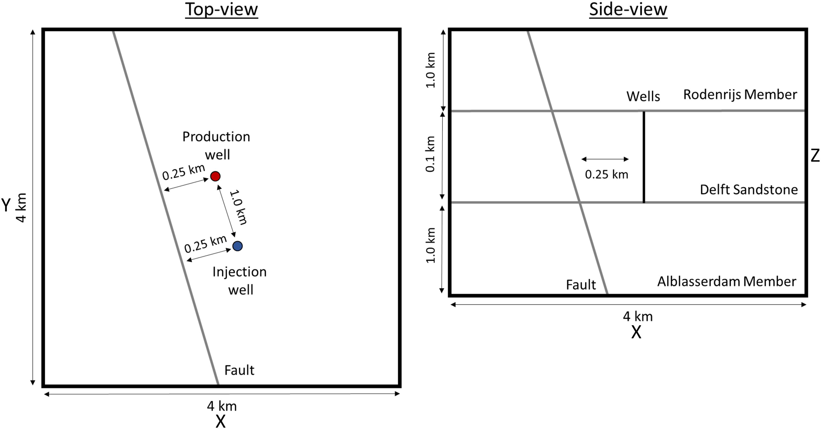
Figure 3. Top (left) and side (right) view of the Delft sandstone model (not to scale).
Table 5. Mechanical, thermal and hydraulic properties of geological units and the fault in the Delft sandstone base case model.

Rock matrix, fault and fluid properties
No consistent literature values were found for Rodenrijs, Delft sandstone and Alblasserdam. Therefore, the values from the Slochteren model were used for Sandstone and Claystone. For the Alblasserdam member approximately average values between Rodenrijs member and Delft Sandstone member were used.
Compared to the Slochteren reservoir, the Delft sandstone member has a higher permeability. The top and bottom layers have a higher porosity. Thermophysical properties of the Delft sandstone layer were based on the Slochteren sandstone model and adapted based on Willems et al. (Reference Willems, Vondrak, Mijnlieff, Donselaar and Van Kempen2020). Rodenrijs properties were based on the claystone properties from the Slochteren model and Alblasserdam properties were based on a mix between sandstone and claystone properties with specific information taken from Willems et al. (Reference Willems, Vondrak, Mijnlieff, Donselaar and Van Kempen2020). For the Delft sandstone model, the same fault properties as in the Slochteren sandstone model were used. Due to the lack of reservoir fluid data, we assume pure water as representative reservoir fluid for the Delft sandstone model.
Besides the base case Delft sandstone model, a small sensitivity analysis is performed for re-injection temperature and well-to-fault distance.
Dinantian limestone reservoir models
The Dinantian carbonate formation is the deepest formation we consider in our analysis. Here, we simplify the geology to a horizontal Limburg claystone layer as top seal, a horizontal Dinantian limestone layer as reservoir layer and a horizontal Devonian claystone-sandstone layer as bottom seal. Due to the low permeability of the rock matrix, we consider three models for geothermal exploitation of the Dinantian limestone: (a) wells intersect a high permeability fault (‘Dinantian fault model’), (b) wells intersect a fault zone (‘Dinantian fault damage zone model’) and (c) hydraulically fractured parallel horizontal wells are drilled next to the fault representing a multi-stage EGS (‘Dinantian EGS model’).
Model geometry and boundary conditions
The depth of the Dinantian varies between 2 and 9 km. For the considered Ultra Deep Geothermal development with temperatures >120°C, we use a 4.5 km deep Dinantian reservoir top. A thickness of 500 m is assumed. The same thickness is used for the top and bottom layers. Fault geometry and properties are the same as in the Slochteren model. All stress, pressure and temperature initial and boundary conditions are the same as in the Slochteren model adapted for the depth.
Operational and wellbore data is the same as in the other two models except that for one scenario, the two deviated wells are 1000 m apart and intersect the fault, and in another scenario two horizontal wells parallel to the minimum horizontal stress direction are 500 m apart and hydraulically connected by five hydraulic fractures with a spacing of 200 m. The distance between wells and fault is here 250 m.
Three models are setup for the Dinantian reservoir. Due to the low reservoir permeability geothermal exploitation needs to focus on existing fault zones (Scenarios S37 and S38) or stimulated fractures (Scenario S39). Figures 4, 5 and 6 display the geometries of the Dinantian limestone reservoir models.

Figure 4. Top (left) and side (right) view of the Dinantian limestone fault model (not to scale).

Figure 5. Top (left) and side (right) view of the Dinantian fault damage zone model (not to scale).
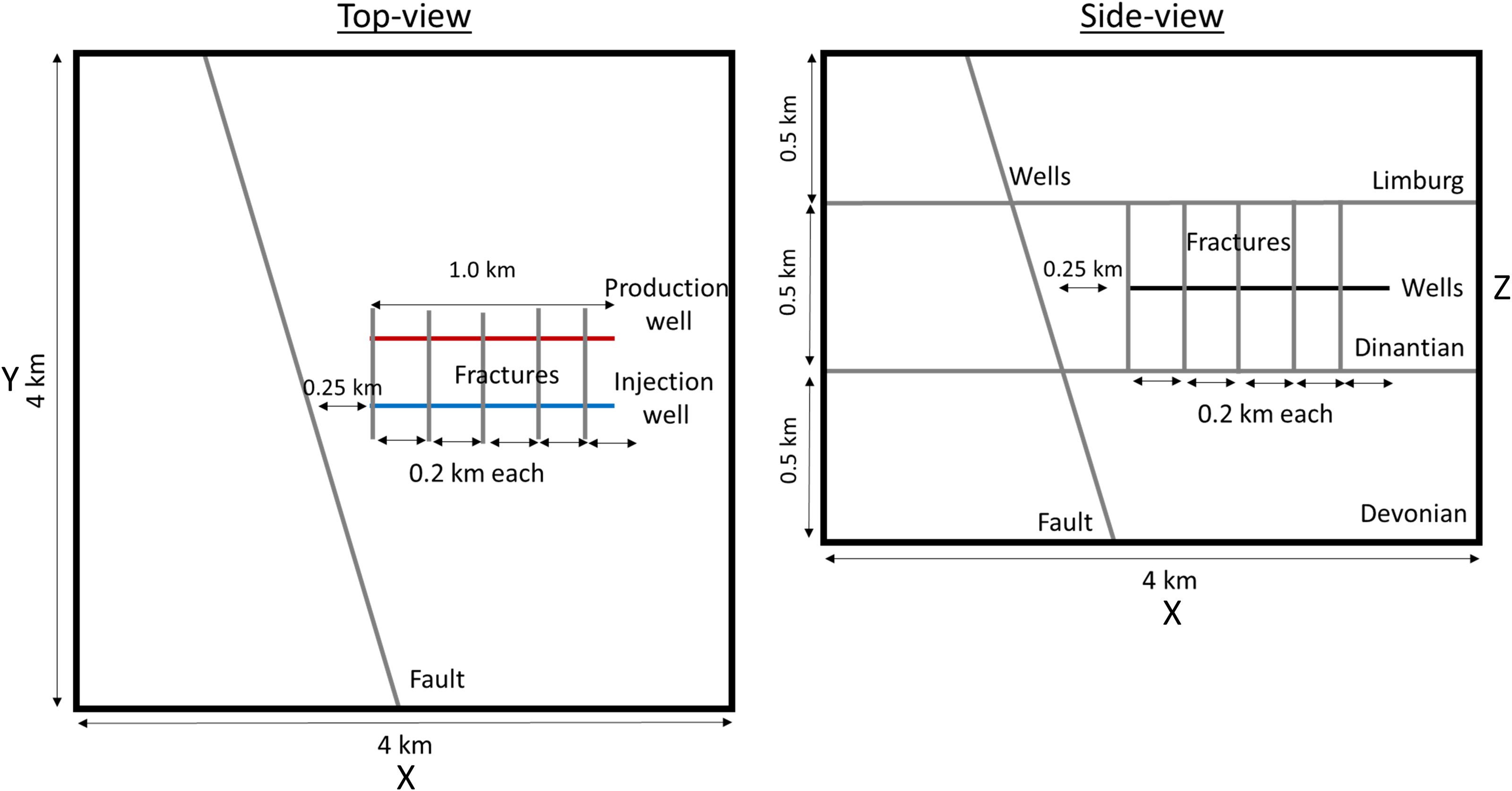
Figure 6. Top (left) and side (right) view of the Dinantian EGS model (not to scale).
Rock matrix, fault and fluid properties
The description of the Limburg properties can be found in the respective sections on the Slochteren model. The Devonian properties are an approximate average of claystone and sandstone and thus correspond to the Alblasserdam Member as defined above for the Delft model. For the Dinantian, typical values for limestone were used when no specific reservoir information was available (Table 6).
Table 6. Mechanical, thermal and hydraulic properties of geological units and the fault/fractures in the Dinantian limestone base case model.

Geomechanical rock properties
For the Dinantian limestone, a Young’s modulus of 40 GPa and a Poisson’s ratio of 0.2 were used according to the value for the Carboniferous in Lele et al. (Reference Lele, Garzon, Hsu, DeDontney, Searles and Sanz2015). According to Schmitt (Reference Schmitt and Schubert2015), the solid bulk moduli of Calcite and Dolomite are 73.3 GPa and 94.9 GPa, respectively. Assuming a calcite dominated limestone, we use a value of 80 GPa. The resulting drained bulk modulus and Biot coefficient are 22.2 GPa and 0.72, respectively.
Hydraulic rock properties
The Dinantian is a low porosity and low permeability limestone formation. Similar or even lower values can be expected for the top and bottom layers. Flow is governed by fracture flow.
Thermophysical rock properties
According to Fuchs et al. (Reference Fuchs, Balling and Förster2015), Calcite and Dolomite have a thermal conductivity of 3.4 and 5.4 W/m/°C, a heat capacity of 820 and 870 J/kg/°C and a density of 2710 and 2880 kg/m³, respectively. We use values closer to the ones of calcite. Srinivasan (Reference Srinivasan1955) reports similar values of thermal expansion coefficient for calcite and for quartz. Therefore, we use the same value of 30 1e-6/°C for the Dinantian limestone and for the Slochteren sandstone.
Fault and fracture properties
Fracture aperture, based on FMI logs in the Dinantian carbonates, were approximately 110 µm (Broothaers et al., Reference Broothaers, Bos, Lagrou, Harcouët-Menou and Laenen2019; Van Leverink & Geel, Reference Van Leverink and Geel2019). Assuming this fracture aperture to be equivalent to the hydraulic aperture, the cubic law yields a fracture permeability of 1000 mD. Thus, we use the same fault properties as in the Slochteren model except for a higher fault permeability of 1000 mD, a correspondingly higher aperture of 110e-6 m and a higher fault porosity of 100%. The same parameters were used for hydraulic fractures.
Reservoir fluid properties
No fluid information is available for the deep Dinantian limestone formation. We thus use high salinity fluid of the Groß Schönebeck reservoir as formation fluid. This is the same as in the Slochteren model.
Results
Slochteren sandstone
Base case model
With the base case model geometry and parameters, the model showed a potential fault failure after 11.45 years of cold-water injection when the maximum slip tendency on the fault reaches the critical value of 0.6 (Fig. 7). Figure 8 shows the temperature and pressure contours around the injection well and the slip tendency on the fault plane after 30 years of circulation. The slip tendency values increase systematically when the cold thermal front reaches the fault plane. The pressure perturbation due to the injection process on the other hand stabilizes relatively quickly and does play only a secondary role in the slip tendency on the fault plane. Figure 9 illustrates the initial and final absolute stresses, thermal stress, pore-pressure and temperature along x-axis and z-axis across the injection well after 30 years of geothermal operation. The figure shows an increased thermal stresses at the formation boundaries. This occurs due to the higher rock stiffness of the top and the bottom layers. It can also be observed from Fig. 9 that the maximum pore-pressure increase around the injection well is 3.8 MPa. The temperature around the injection well reaches the injection water temperature, that is, 30°C. Thermal stresses generated due to the temperature change affect the mechanical stress state of the rocks. The combined effect of the thermal, hydraulic and mechanical processes results in an increase in the computed slip tendency along the fault. After 30 years of cold water injection, ∼0.077 km2 fault area undergoes failure and the fault plane within the reservoir section experiences a maximum slip tendency of 0.85.

Figure 7. Maximum slip tendency on the fault and fault failure within the reservoir unit of the Slochteren base case model.

Figure 8. Temperature contours (in °C), pressure contours (in MPa) and slip tendency (unitless) on the fault in the Slochteren base case model after 30 years of circulation.

Figure 9. Temperature, pore-pressure and effective stresses (compression is negative) across the injection well (a) along x-axis and (b) along z-axis, initial (dash) and after 30 years (solid) of circulation in the Slochteren base case model.
Sensitivity analysis
To understand the impact of the most important reservoir geometries, geological and operational parameters, a sensitivity analysis was performed (Table 7). The results obtained from the sensitivity analysis cases were only analysed in the reservoir section to ensure the same initial stress state. Figure 10 shows that the parameters that constitute the thermal and mechanical governing equations have the highest impact on the fault failure potential. These parameters included the stress gradients; geo-mechanical reservoir properties like Young’s modulus and Poisson’s ratio; operational and wellbore data such as the distance between the wells and the fault, re-injection temperature, flow rate; other geological properties like temperature and pressure gradients, thermal expansion coefficient, fault dip, reservoir depth and porosity of the reservoir rock. Many of these parameters also impacted the magnitudes of maximum temperature change along the fault (Fig. 11). This indicates a strong correlation between the thermal stresses and the computed slip tendency values as dictated by Equation (3). However, such correlation was not observed with the maximum change in pressure values given in Fig. 12. Parameters such as pore-pressure differential, permeability and fluid viscosity did exert only a minor impact on the slip tendency of the fault, indicating how the hydraulic feedback coupling is not significant to determine the fault failure mechanism. A cross examination of Figs. 10 and 13 indicates that the cases with higher slip tendencies also resulted in a larger area of the fault with a potential to fail. Even by assuming the same amount of slip for the two cases, a larger area would result in a larger seismic moment and therefore in a higher magnitude of the potential induced event assuming that the slip would be seismic. Figure 14 shows that these cases also failed earlier than the cases with low slip tendency values.
Table 7. Modelling scenarios for the Slochteren sandstone, Delft sandstone and Dinantian limestone sensitivity analysis.


Figure 10. Results of the sensitivity analysis for the fault within the reservoir unit: Maximum slip tendency after 30 years of circulation in the Slochteren models.

Figure 11. Results of the sensitivity analysis for the fault within the reservoir unit: Maximum temperature change after 30 years of circulation in the Slochteren models.

Figure 12. Results of the sensitivity analysis for the fault within the reservoir unit: Maximum pore-pressure change after 30 years of circulation in the Slochteren models.

Figure 13. Results of the sensitivity analysis for the fault within the reservoir unit: Fault area with slip tendency exceeding the friction coefficient (0.6) of the fault after 30 years of circulation in the Slochteren models.

Figure 14. Results of the sensitivity analysis for the fault within the reservoir unit: Time to reach the critical slip tendency in the Slochteren models.
One simulation scenario was considered without thermo-elastic effects which resulted in a significant change in the slip tendency on the fault plane. The maximum slip tendency without thermo-elastic effects is only 0.27 instead of 0.85, highlighting the importance of thermal effects on slip tendency in our models. Two special case scenarios were also simulated: (a) a deep low porosity reservoir model and (b) a shallow high porosity reservoir model. The maximum slip tendencies observed in the reservoir layer in these cases after 30 years of geothermal operation were 0.7 and 0.4, respectively, indicating that deep low porosity reservoirs have a higher fault slip potential compared to shallow high porosity reservoirs.
Delft sandstone
Base case model
The Delft sandstone reservoir shows a potential fault failure after 3.95 years of cold-water injection. With 30 years of geothermal operation, the fault plane within the reservoir section experiences a maximum slip tendency of 1 and a fault area of 0.091 km2 potentially undergoes failure. The maximum change in the temperature at the fault section within reservoir unit is 54.2°C. As compared to the Slochteren sandstone base case model, the Delft sandstone model experienced a higher slip tendency and a quicker fault failure (Table 8). This can be attributed to the difference in the geometry of the two models. A smaller reservoir thickness of the Delft reservoir leads to a wider distribution of the thermal front.
Table 8. Comparison of Slochteren, Delft and Dinantian EGS models.

Sensitivity analysis
A sensitivity analysis was performed for different re-injection fluid temperatures: (a) 15°C, (b) 30°C (base case) and (c) 45°C. With 15°C re-injection temperature, the rock matrix experiences higher thermal stresses as compared to the base case and thus fault failure occurs earlier at 3.15 years. The change in temperature at the fault surface after 30 years is 69.6°C with a failure area of 0.10 km2. The scenario with re-injection water temperature of 45°C, on the other hand, experiences lower thermal stresses as compared to the base case. The fault failure occurs after 6.45 years. The maximum temperature change on the fault plane after 30 years is 38.8°C, and the critically stressed fault area is 0.056 km2.
In another sensitivity analysis scenario, the distance between the injection well and the fault was increased to 500 m. In this case, the fault failure was not observed within the operational period of 30 years. The maximum slip tendency was observed to be 0.51, the maximum temperature change on the fault to be 84.4°C and the maximum pressure change on the fault was 84.1 MPa.
Dinantian limestone
Fault-dominated exploitation
In the Dinantian base case model and the Dinantian damage zone model, the injection and production wells intersect the fault. In both the cases, fault failure is observed at the beginning of circulation. Figure 15 shows the cross-sections across the injection wells in each case. The injection water flows outwards into the reservoir unit in the base case model, whereas in the damage zone model, the cold injection water flows primarily through the fault damage zone also intersecting the top and bottom units.

Figure 15. Comparison of temperature distribution after 30 years of circulation in the (a) Dinantian fault model and (b) the Dinantian damage zone model.
Enhanced Geothermal Systems (EGS)
As compared to the fault-dominated exploitation of the Dinantian limestone reservoir, the EGS models shows significantly lower potential of fault failure. The injected water in the EGS models is distributed into the reservoir unit through the hydraulic fractures. As a result, the temperature changes primarily affect the immediate vicinity of the injection well and have little impact on the stress changes occurring on the fault plane. Figure 16 shows the slip tendency on the fault plane in the EGS models after 30 years of circulation. The EGS system with 500 m distance between the injection well and the fault shows no failure potential, whereas the EGS model with 250 m distance between the injection well and the fault shows failure potential after 28.7 years.

Figure 16. Comparison of temperature distribution on hydraulic fractures and slip tendency on the fault after 30 years of circulation in (a) the Dinantian EGS model with 250 m well-fault spacing and (b) 500 m well-fault spacing.
Discussion
The study suggests that for the given assumptions and boundary conditions, the changes in the slip tendency of a fault (2D planar discontinuity with zero cohesion) can largely be attributed to thermo-mechanical effects. Once a new equilibrium is reached in a doublet system after a few months, the direct influence of pore pressure on slip tendency remains constant, while the cold-water front will continue to expand around the injection well for as long as the well is in operation. A significant increase in the slip tendency was observed when this low temperature front reached the fault zone. Besides the obvious importance of the stress field and the local fault geometry, rock mechanical properties and operating conditions have a major influence on the induced stress changes and the related fault activation potential triggered by geothermal operations. Thus, careful selection of a suitable target formation and the operational parameters is crucial to minimize the risk of induced seismicity. The most important geological parameters that should be known while selecting the geothermal site are the regional stress gradients, temperature gradient, pressure gradient, geo-mechanical properties of the reservoir layer such as the Young’s modulus and Poisson’s ratio, thermal expansion coefficient of the formation, fault orientation, reservoir porosity, depth and thickness of the reservoir layer. Lower stress, temperature and pressure gradients, lower reservoir rock stiffness, shallower depth, higher reservoir porosity, larger reservoir thickness, lower thermal expansion coefficient and higher fault dip contribute to a low risk geothermal environment. Besides selecting a low-risk geothermal formation, the failure potential can further be minimized by optimizing operational parameters. The key planning and operational parameters to be considered include the distance between the injection well and existing known faults, re-injection temperature and injection flow rate. During the geothermal operations, the most effective measures to reduce the risk of induced seismicity are increasing the re-injection temperature and decreasing the injection rate. The EGS system with optimized well-to-fault distance can be an effective technique for the mitigation of induced seismicity in deeper reservoirs such as Dinantian limestone.
In this study, we did not consider fault offsets to avoid further complexity in the interpretation of the results and numerical artefacts in the form of stress concentrations on sharp geometrical edges, which are not found in reality, as described before. With a fault offset of less than 200 m (hydraulic connection between reservoir formation on both sides of the fault), the effect would be similar to the results of the sensitivity analysis of the reservoir thickness. Within the 0–200 m range, a larger fault offset would lead to a pressure increase and temperature reduction on the fault, leading to earlier fault slip and increasing slip tendencies. With larger fault offsets, the impermeable Limburg claystone formation on the other side of the fault would prevent flow and convective heat transfer across the fault, leading to higher pressures, but significantly less temperature changes on the fault and thus significantly lower slip tendencies. This case would thus be similar to the impermeable fault scenario.
We note again that although the slip tendency may indicate fault reactivation, it does not tell anything about the seismicity to be expected from this fault failure. Therefore, we performed an additional analysis by applying the rate-and-state friction (RSF) formalism to the same model to get some information about the dynamics of a potential fault slip (Supplementary material S1). The empirical constants describing the frictional properties of the fault in the RSF framework were taken from Hunfeld et al. (Reference Hunfeld, Niemeijer and Spiers2017). The RSF parameters provided in the cited study were determined by direct shear experiments performed on simulated Slochteren sandstone fault gouges. These experiments did not include fluid injection and did not consider the effect of long-term thermal stressing of the samples. Nevertheless, based on Hunfeld et al. (Reference Hunfeld, Niemeijer and Spiers2017), the Slochteren sandstone fault gouges show velocity strengthening behaviour in the direct shear experiments, and consequently our RSF model also resulted in slow, stable slip, which might be an indicator for aseismic slip (Guglielmi et al., Reference Guglielmi, Cappa, Avouac, Henry and Elsworth2015). Hunfeld et al. (Reference Hunfeld, Niemeijer and Spiers2017) have also indicated that the overlying Zechstein formation shows velocity weakening characteristics. Since in our model the pore pressure and cooling-induced stress changes are mainly limited to the fault area overlapping with the reservoir layer (see Fig. 8), we neglected the potentially different friction behaviour of the Zechstein caprock and characterized the entire fault with a single parameter set. This choice is justified by the fact that no significant seismicity (i.e. Mw > 2) is observed in the hydrothermal systems of the Netherlands and the velocity strengthening behaviour of the faults in these reservoirs could be one potential reason for this. Nevertheless, faults in the Netherlands may also exhibit velocity weakening behaviour and adapting the RSF parameters in our model accordingly would lead to seismic rather than a seismic slip. A thorough analysis of the frictional behaviour of reactivating faults in the Slochteren Sandstone formation (related to geothermal operation) has to be the subject of future studies based on field observation and site-specific geological models.
A limitation of the current model is the lack of validation with field observations from the Netherlands due to the lack of data. No induced seismicity has been observed in the conventional matrix-type geothermal reservoirs in the Netherlands, whereas a previously observed induced seismicity in the Dinantian limestone reservoir indicates the need of a detailed analysis of the geological and operational settings of EGS systems.
We note that we have chosen a simplified approach to include the Zechstein formation in our simulations by modelling it as a homogeneous linear elastic layer without considering secondary creep mechanism. This was done intentionally to avoid further model complexity since this study focuses mainly on the fluid injection induced seismicity inside the respective reservoir layers. In addition, considering the Zechstein formation as a homogeneous viscoelastic layer that consists of pure rock salt would also be a similarly strong assumption. However, it was shown in the case of the Groningen gas field that the presence of the viscoelastic Zechstein caprock can contribute to depletion-induced seismic slip (Wassing et al., Reference Wassing, Buijze, Ter Heege, Orlic and Osinga2017; Candela et al., Reference Candela, Osinga, Ampuero, Wassing, Pluymaekers, Fokker, van Wees, de Waal and Muntendam-Bos2019).
Therefore, the absolute values for slip tendency, failure area, temperature and pressure should be interpreted considering the limitations and assumptions of our model. Nevertheless, the absolute values demonstrate how the calculated slip tendency for this model changes when the input parameters are changed within realistic ranges that apply to the Netherlands.
Potential future studies can include site-specific model geometries, further refined meshes, a nonlinear failure criterion, poro-elastic coupling and a creep constitutive law for the Zechstein salt. It has to be noted that implementing more realistic fault systems (e.g. en echelon segmented) will have a major impact on the individual interplay of key impact factors and resulting slip and induced seismicity patches along the fault.
Conclusions
Our results of Dutch geothermal well doublet THM models indicate that thermal effects can play a major role in fault stability, supporting the observations of recent numerical modelling studies (Wassing et al., Reference Wassing, Candela, Osinga, Peters, Buijze, Fokker and Van Wees2021; Kivi et al., Reference Kivi, Pujades, Rutqvist and Vilarrasa2022). Cooling-induced thermal stresses cause tensile stresses, thereby reducing the magnitude of the resulting compressive stresses. This increases the slip tendency of the fault. Thermal stresses are highly sensitive to geo-mechanical reservoir rock properties, for example, Young’s modulus and Poisson’s ratio. The higher the rock stiffness, the higher the chances of failure during cold fluid injection. Within the range of investigated geometries, the Slochteren sandstone exhibits a more stable fault configuration when characterised by a higher fault dip and a fault strike that is oriented at a greater angle relative to the SHmax direction. According to the sensitivity analysis, a significant variation in stress gradients across different principal directions corresponds to elevated shear stresses, which increases the potential for fault failure. Among the thermal properties, bulk thermal expansion coefficient has the most significant effect on fault stability. Well-to-fault distance, re-injection temperature and injection flow rate are key parameters that can influence the seismic risk. Therefore, it is essential to carefully consider these parameters when planning a geothermal system. In the case of typical Slochteren deep geothermal systems, hydraulic parameters and fluid properties such as rock permeability, fluid viscosity and fluid density have minor impact on fault stability within their respective investigated ranges.
Supplementary material
The supplementary material for this article can be found at https://doi.org/10.1017/njg.2023.12
Acknowledgements
The authors are grateful for the financial support provided by the ‘Kennis Effecten Mijnbouw’ (KEM)-programme through the project ‘Risk of seismicity due to cooling effects in geothermal systems – KEM-15’, and input from Staatstoezicht op de Mijnen (SodM, Dutch State Supervision on Mines), particularly Richard Bakker, Niels Grobbe and Annemarie Muntendam-Bos. We also thank FUGRO for providing the expertise on the geological background. We kindly acknowledge the financial support of the Helmholtz Association’s Initiative and Networking Fund for the Helmholtz Young Investigator Group ARES (contract number VH-NG-1516).
Authors’ contributions
BM set up and carried out all simulations presented in the manuscript. HH gathered and compiled the reservoir and fluid data and supervised the study, MC helped set up and troubleshoot the simulation input files, GH supported the mesh refinement and time step optimization and performed the RSF analysis in the supplementary material and AZ supervised the study. All authors collaborated on the writing.
Competing interests
The authors declare no competing interests.


 Open access