


1. Introduction
For many low-income food deficit countries (LIFDCs),Footnote 1 swings in staple food prices are an important source of macroeconomic instability. Theory suggests that in the face of instable current accounts, attributable to relatively volatile export earnings and/or import bills, agents should seek to enhance savings, a move that enables smoothing consumption over time (Ghosh and Ostry, Reference Ghosh and Ostry1994). Still, the ability to increase the level of savings is rather limited in many poor net food importing developing countries, mainly because of weak domestic financial systems. Countries can also try to borrow funds from international markets to finance import requirements, thus balancing a current account deficit with higher capital inflows. This is possible provided countries still have the ability to sustain additional borrowing without prompting a rise in default risks.
In this context of limited access to savings and borrowing, cash crop export earnings can act as an automatic consumption smoothing mechanism for LIFDCs. This is because international demand for agricultural commodities (including cash crops) is generally inelastic, implying that movements in prices outweigh those of quantities (Food and Agriculture Organization of the United Nations [FAO], 2004). Hence, rising cash crop and staple food prices translate into increasing export earnings and import bills. A casual review of price data series shows that staple food and cash crop quotations tend to display synchronized behavior. For example, during the recent commodity price surge episode, wheat and rice prices went up by 17% and 65%, between 2006 and 2009, respectively, while international prices for coffee, tea, and sugar, grew by 26%, 45%, and 23%, over the same period, respectively.Footnote 2 Overall, between 2002 and 2008, the World Bank agricultural subindex increased by 102.9%. The rise in cash crop prices, together with staple food prices, means that export revenues from the commodities that many LIFDCs rely on could act as a good hedge against surges in food import bills and contribute to reducing current account instability.Footnote 3
This study looks at one particular aspect of current account instability that relates to the extent to which changes in cash crop prices can dampen the effect of higher food prices.Footnote 4 We explore the price relationship by examining comovements and dynamics in terms of price level and volatility. Although movements in quantities together with prices determine the direction and magnitude of export earnings, the focus in this article is exclusively on the price component of the equation given its relative importance. Volatility is important to study because it helps shed some light on the transmission of information/uncertainty from one market to another. Research also indicates that the prevalence of high volatility hinders investment and planning.
In order to gain further insights into the staple food–cash crops price relationship, we apply a wavelet analysis to decompose the series into three timescale levels corresponding to the short, medium, and long run. That is because policy implications differ depending on the nature of the price linkages at each time horizon. For instance, if the price dynamics are stronger in the long run, as opposed to the short run, cash crop earnings could potentially limit, or offset, rises in international food prices, whereas in the short run, measures may be required to address current account imbalances. Further, the application of wavelet analysis enables the detection of breaks or any sudden changes in the dynamics that may characterize the series.
After decomposing the series, a multivariate Baba, Engle, Kraft, and Kroner (BEKK)–generalized autoregressive conditional heteroskedasticity (GARCH) framework (Engle and Kroner, Reference Engle and Kroner1995) is applied to explore the dynamics of the volatility interaction and conditional correlation at various frequency levels. The advantage of using the BEKK framework is that it ensures a symmetric and positive definite conditional variance-covariance matrix. In addition, the model produces fewer parameter estimates compared with other multivariate GARCH (MGARCH) models when evaluating volatility transmission across markets (Gardebroek and Hernandez, Reference Gardebroek and Hernandez2013). To minimize the effect of model convergence issues that are often associated with BEKK-GARCH parameterization, we construct two price indices that we use for the estimation exercise. The first price index captures daily futures price changes for sugar, cotton, cocoa, and coffee and is referred to as the cash crop price index. The second index depicts daily futures price changes for wheat, maize, and soybeans and represents the staple food crop price index. Both price indices are volume weighted, with data on daily volumes obtained from the futures markets where the commodity is traded.Footnote 5 The idea of weighting by volume is to give prominence to the commodities in the price index that are traded the most.Footnote 6 Note that the data show a jump in the assigned weights as the contract expiry date nears. Nonetheless, these changes do not alter the relative importance of specific commodities in the index. That is, sugar and maize remain the most traded contracts regardless of the changes in weights because of the effect of expiring contracts. Scaling the estimated conditional covariances by the estimated conditional variances yields a series of conditional correlations, which permit the examination of conditional correlation patterns between the cash crop and staple food indices at different timescales.
In addition to easing model convergence, undertaking the analysis at the aggregate level offers some insights into the relationship between cash crop and staple food international prices, before deciding on whether it is “worth” exploring further the analysis at the country level, given the challenges associated with the data. Indeed, data series on cash crop and staple food prices for developing countries are often short, contain missing values, and are generally available at low frequency only, which makes it difficult to obtain robust results using a BEKK-GARCH approach.
Our research contributes to the literature in four aspects. First, as opposed to the bulk of the existing studies on the relationship between staple foods and cash crops, we examine the price level and volatility interaction from a global perspective. Hence, we contribute to providing evidence-based analysis of the potential contribution of cash crop export earnings to food import bills, particularly during periods when food prices are relatively high and volatile. Second, we use wavelet transforms to decompose the price series into different timescales, enabling an assessment of volatility dynamics otherwise hidden in the original series. Third, we estimate conditional correlations between cash crops and staple food indices at difference time frequency domains. This way, we evaluate the potential dampening effect of cash crop export earnings on current account variability because of rising food import prices. Finally, the literature on the linkages between balance of payments and commodity export/import is quite substantive, with marked contributions from international organizations, including the FAO (2016), the International Monetary Fund (IMF, 2008), and the United Nations Conference on Trade and Development (UNCTAD and FAO, 2017). As if often the case, member countries of these organizations (notably through the Group of 77, an intergovernmental group of developing countries) request that normative work be carried out on this topic, given its practical relevance. This article adds to that research stream.
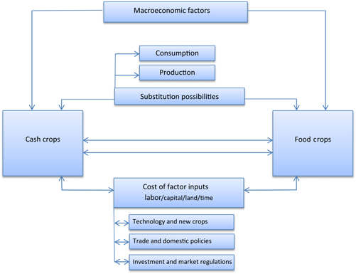
We should note that the observed synchronized movement between cash and staple food international prices cannot be explained by market fundamentals only, at least in the short term. That is because the substitution possibility in consumption and production between cash crops and staples in the physical market is limited and, hence, cannot explain the extent of price correlation. On the other hand, macroeconomic shocks, weather impacts affecting major producers of both commodity groups, changes in energy prices, and the potential influence of institutional investors could cause futures prices to comove. The influence of institutional investors on commodity markets still remains ambiguous (Fattouh, Kilian, and Mahadeva, Reference Fattouh, Kilian and Mahadeva2012; Hamilton and Wu, Reference Hamilton and Wu2015; Irwin and Sanders, Reference Irwin and Sanders2011). A causal attribution analysis is beyond the scope of this study. Figure A2 (see Appendix) describes the main linkages between cash crop and staple food markets and some of the possible factors underlying the relationship.
The rest of the article is organized as follows: Section 2 covers a short review of relevant studies on cash crops and staples and the use of the GARCH methodology. We then present a discussion on the methodology and data used in the analysis (Section 3), followed by a discussion about the main empirical results and observations (Section 4). Finally, a summary of the main conclusions and implications is provided in Section 5.
2. Literature review
The literature on the relationship between international staple food and cash crop prices is mostly concerned with farm resource allocation and, precisely, whether cash crop production and export compete for resources with food crop production. The concern is that a focus on cash crop production may create some risks for smallholder farm households, notably in terms of food security. One school of thought argues that cash crop production is detrimental to food security (Maxwell and Fernando, Reference Maxwell and Fernando1989; Mittal, Reference Mittal2009), whereas others contend that a cash crop strategy improves farm welfare because proceeds from cash crops provide the means to buy food in the local market (i.e., the access dimension of food security) (Timmer, Reference Timmer1997; Von Braun and Kennedy, Reference Von Braun and Kennedy1986; Weber et al., Reference Weber, Staatz, Crawford, Bernsten and Holtzman1988). Recent papers in this field claim that staple foods and cash crops should be viewed as complementary rather than competitive. By participating in cash crop schemes, smallholders can have access to productivity enhancing inputs such as credits, management training, fertilizers, and other factor inputs that would not have been available without the participation in cash crop programs (Govereh and Jayne, Reference Govereh and Jayne2003; Theriault and Tschirley, Reference Theriault and Tschirley2014).
Although many studies provide some interesting insights into the mechanisms that explain the allocation of farm resources to the production of cash crops by smallholders in developing countries (Norton and Hazell, Reference Norton and Hazell1986), they seldom address the interaction of cash crop and staple food prices at the international market level. The dynamics at the international level are relevant because they often determine movements in domestic prices. For example, coffee prices received by farmers in Ghana are associated with futures prices negotiated at the Intercontinental Exchange (ICE) market in New York. Similarly, wheat imports prices paid by Egypt, the world’s largest wheat importer, are linked with wheat futures prices such as those negotiated at the Chicago Board of trade (CBOT) or Euronext/Matif in Paris (Janzen and Adjemian, Reference Janzen and Adjemian2017). Hence, the benefit of specializing in cash crop production, and the use of revenues to import food, hinges on the interaction of cash crop and staple food futures prices. High exports revenues can help alleviate partially, or fully, the burden associated with food import bills during periods of high international food prices. The extent of the contribution depends on several factors, which include the contribution of cash crop earnings to total export revenues, the price elasticities of international demand and supply for cash crops, and currency movements.
Whereas the available research into the volatility dynamics between cash crop and staple food international prices is relatively limited, studies using GARCH methodology to assess the interdependence among markets, including agriculture, are quite prolific. For example, Vivian and Wohar (Reference Vivian and Wohar2012) use a GARCH approach to examine the volatility interaction among a sample of 28 commodities and find significant volatility linkages and volatility persistence even after taking structural breaks into account. Using a BEKK and a dynamic conditional correlation (DCC) trivariate GARCH approach, Gardebroek and Hernandez (Reference Gardebroek and Hernandez2013) find evidence of unidirectional volatility spillover running from maize to ethanol, but weak evidence of transmission from crude oil to maize market in the United States. An MGARCH with structural breaks is applied by Teterin et al. (Reference Teterin, Brooks and Enders2016) to explore the volatility dynamics between crude oil and maize future prices. Their results show that the volatility between crude oil and maize is less persistent when accounting for structural breaks in the mean and volatility. In a recent study, Al-Maadid et al. (Reference Al-Maadid, Caporale, Spagnolo and Spagnolo2017) conclude that there are significant volatility spillover effects between energy and food markets, with the interaction greater during the 2006 food crisis and the 2008 financial crisis. Other studies using a GARCH method to examine price volatility among various commodities include those by Chang and Su (Reference Chang and Su2010), Ji and Fan (Reference Ji and Fan2012), Harri and Hudson (Reference Harri and Hudson2009), de Nicola et al. (Reference de Nicola, De Pace and Hernandez2016), and Trujillo-Barrera et al. (Reference Trujillo-Barrera, Mallory and Garcia2012).
A growing number of studies looking at agricultural price volatility have been using wavelet-based techniques. Although these techniques are common in the fields of physics, medicine, and mathematics, the expansion of their application to economics and finance is a quite recent phenomenon. The advantage of this approach is that it allows a decomposition of the main components of a price series to gain additional insights into the underlying factors shaping their movements (Percival et al., Reference Percival, Wang and Overland2004). For example, Filip et al. (Reference Filip, Janda, Kristoufek and Zilberman2016) apply a wavelet analysis to study the linkages between the price of feedstocks and ethanol in both Brazil and the United States. Their results show that feedstock prices lead those of ethanol. Kristoufek et al. (Reference Kristoufek, Janda and Zilberman2016) report similar results using a wavelet coherence approach. Mensi et al. (Reference Mensi, Tiwari, Bouri, Roubaud and Al-Yahyaee2017) combine a wavelet and copula method to examine the interaction between implied volatility indices for oil, wheat, and maize and find evidence of asymmetric tail dependence among the selected commodities. Also, using a wavelet approach to disentangle the interaction between commodity and credit markets in sub-Saharan Africa, Ftiti et al. (Reference Ftiti, Kablan and Guesmi2016) find a strong relationship over long timescales, confirming that the credit market is affected by persistent commodity shocks. Power and Turvey (Reference Power and Turvey2010) use a wavelet method to study the volatility interaction among 14 commodities, and Pal and Mitra (Reference Pal and Mitra2017) using a wavelet-based methodology find that world food prices comove with crude oil prices, with the latter leading world food quotations.
With increasing evidence linking the market performance of equities to changes in commodity prices, several studies analyze the interaction between the financial market and commodities, including agriculture. These studies provide empirical evidence explaining the comovement between financial markets and commodities. The use of GARCH-based techniques in these studies is very common. For example, Mensi et al. (Reference Mensi, Beljid, Boubaker and Managi2013) examine the volatility integration between energy, food, gold, and beverages price indices, and the U.S. S&P 500 index. Their results show significant return and volatility transmission across markets. Gao and Liu (Reference Gao and Liu2014) use a bivariate GARCH model to investigate the volatility interdependence between the S&P 500 index and a sample of commodities, and Nazlioglu et al. (Reference Nazlioglu, Erdem and Soytas2013) look at the volatility transmission between crude oil and agricultural commodity markets, evidencing significant mean return and volatility integration. Other studies examining the linkages between financial markets and commodities include those by Olson et al. (Reference Olson, Vivian and Wohar2014), Park and Ratti (Reference Park and Ratti2008), Awartani and Maghyereh (Reference Awartani and Maghyereh2013), El Hedi Arouri et al. (Reference El Hedi Arouri, Jouini and Nguyen2011), Malik and Ewing (Reference Malik and Ewing2009), Diebold and Yilmaz (Reference Diebold and Yilmaz2012), Amatov and Dorfman (Reference Amatov and Dorfman2017), and Grosche and Heckelei (Reference Grosche, Heckelei, Kalkuhl, von Braun and Torero2016).
3. Methodology and data
3.1. Wavelet analysis
Wavelet analysis is used to decompose a signal into its main components, enabling the possibility to focus on specific frequencies (Percival et al., Reference Percival, Wang and Overland2004). In contrast to the Fourier transform, wavelet transform combines information on both time and frequency domains, allowing us to track timewise particular frequencies (Mensi et al., Reference Mensi, Tiwari, Bouri, Roubaud and Al-Yahyaee2017). A wavelet transform is based on the mathematical operation of convolution, which specifies that the integral of the product of two functions, one of which is reversed and shifted, produces a third function that has similar features as the shifted and reversed function (Torrence and Compo, Reference Torrence and Compo1998). The wavelet transform is based on two specific functions: (1) the father wavelet, ϕ(t), and (2) the mother wavelet, Ψ(t). A series of wavelets called daughter wavelets, Ψ u,s (t), can be built by simply scaling and translating (shifting) Ψ(t):
 $${{\rm{\Psi }}_{u,s}}\left( t \right) = {1 \over {\sqrt s }}{\rm{\Psi }}({{t - u} \over s}),$$
(1)
$${{\rm{\Psi }}_{u,s}}\left( t \right) = {1 \over {\sqrt s }}{\rm{\Psi }}({{t - u} \over s}),$$
(1)
where ${1 \over {\sqrt s }}$
is a normalization factor ensuring unit variance of the wavelet (i.e., ||Ψ
u,s
(t)||2 = 1), and u and s are the location and scaling parameters, respectively (Crowley, Reference Crowley2005). The scaling parameter controls for the length of the wavelet and is related to the frequency of the input signal such that a larger (lower) value implies the wavelet will correlate with the low (high) frequencies contained in the time series. The term u determines the location of the wavelet in the time domain. A number of wavelets have been developed to capture specific frequency characteristics of time series, and these include the Daubechies, Haar, Morlet, and Mexican hat. There are two types of wavelet transforms that are widely used in the literature: (1) the discrete wavelet transform (DWT) and (2) the continuous wavelet transform (CWT) (Crowley, Reference Crowley2005). The DWT is suitable for data compression and noise reduction, whereas the CWT is useful for smooth extraction of frequencies. Mother wavelets have to satisfy two main conditions: (1) zero mean (i.e.,
${1 \over {\sqrt s }}$
is a normalization factor ensuring unit variance of the wavelet (i.e., ||Ψ
u,s
(t)||2 = 1), and u and s are the location and scaling parameters, respectively (Crowley, Reference Crowley2005). The scaling parameter controls for the length of the wavelet and is related to the frequency of the input signal such that a larger (lower) value implies the wavelet will correlate with the low (high) frequencies contained in the time series. The term u determines the location of the wavelet in the time domain. A number of wavelets have been developed to capture specific frequency characteristics of time series, and these include the Daubechies, Haar, Morlet, and Mexican hat. There are two types of wavelet transforms that are widely used in the literature: (1) the discrete wavelet transform (DWT) and (2) the continuous wavelet transform (CWT) (Crowley, Reference Crowley2005). The DWT is suitable for data compression and noise reduction, whereas the CWT is useful for smooth extraction of frequencies. Mother wavelets have to satisfy two main conditions: (1) zero mean (i.e., ${\rm{}}\mathop \int \noilimits_{ - \infty }^\infty {\rm{\Psi }}\left( t \right)dt = 0$
) and (2) unit energy (localized in time or space; i.e.,
${\rm{}}\mathop \int \noilimits_{ - \infty }^\infty {\rm{\Psi }}\left( t \right)dt = 0$
) and (2) unit energy (localized in time or space; i.e., $\mathop \int \nolimits_{ - \infty }^\infty {{\rm{\Psi }}^2}\left( t \right)dt = 1$
). In addition, wavelets have to satisfy the admissibility condition, which guarantees a reconstruction of the original time series from its wavelet transform using the inverse transform (Shalini and Prasanna, Reference Shalini and Prasanna2016). For this article, we use the DWT, given the flexibility it offers in denoising time series (Crowley, Reference Crowley2005), but also because it produces a minimum number of coefficients necessary to reconstruct a series. Given its parsimonious nature, the DWT has wide applications (Moya-Martínez et al., Reference Moya-Martínez, Ferrer-Lapeæa and Escribano-Sotos2015). To minimize the boundary effects at the extremities of time series when applying the DWT, we use the periodic decomposition often done in similar studies. Based on the DWT, any time series can be described as a linear combination of father and mother wavelets (Mensi et al., Reference Mensi, Tiwari, Bouri, Roubaud and Al-Yahyaee2017):
$\mathop \int \nolimits_{ - \infty }^\infty {{\rm{\Psi }}^2}\left( t \right)dt = 1$
). In addition, wavelets have to satisfy the admissibility condition, which guarantees a reconstruction of the original time series from its wavelet transform using the inverse transform (Shalini and Prasanna, Reference Shalini and Prasanna2016). For this article, we use the DWT, given the flexibility it offers in denoising time series (Crowley, Reference Crowley2005), but also because it produces a minimum number of coefficients necessary to reconstruct a series. Given its parsimonious nature, the DWT has wide applications (Moya-Martínez et al., Reference Moya-Martínez, Ferrer-Lapeæa and Escribano-Sotos2015). To minimize the boundary effects at the extremities of time series when applying the DWT, we use the periodic decomposition often done in similar studies. Based on the DWT, any time series can be described as a linear combination of father and mother wavelets (Mensi et al., Reference Mensi, Tiwari, Bouri, Roubaud and Al-Yahyaee2017):
 $${{X}}\left( t \right) = \mathop \sum \limits {_ks_{j,k}}{{\rm{\Phi }}_{j,k}}\left( t \right) + \mathop \sum \limits {_kd_{j,k}}{{\rm{\Psi }}_{j,k}}(t) + \ldots + \mathop \sum \limits {_kd_{1,k}}{{\rm{\Psi }}_{1,k}}(t),$$
(2)
$${{X}}\left( t \right) = \mathop \sum \limits {_ks_{j,k}}{{\rm{\Phi }}_{j,k}}\left( t \right) + \mathop \sum \limits {_kd_{j,k}}{{\rm{\Psi }}_{j,k}}(t) + \ldots + \mathop \sum \limits {_kd_{1,k}}{{\rm{\Psi }}_{1,k}}(t),$$
(2)
where j represents the multiresolution, or scale level, and k depicts the number of coefficients at each scale level. Further, sj,k and dj,k are the scaling (or smooth) and detail (or wavelet) coefficients, respectively, and can be expressed as
 $${s_{j,k}} = \mathop \vint \nolimits X(t){{\rm{\Phi }}_{j,k}}\left( t \right)dt,\,\rm and$$
(3)
$${s_{j,k}} = \mathop \vint \nolimits X(t){{\rm{\Phi }}_{j,k}}\left( t \right)dt,\,\rm and$$
(3)
 $${d_{j,k}} = \mathop \vint \nolimits X(t){{\rm{\Psi }}_{j,k}}(t)dt,{\rm{ for \it{\ j} }} = {\rm{ 1}},{\rm{ 2}},{\rm{ }} \ldots ,{\it{ j}}.$$
(4)
$${d_{j,k}} = \mathop \vint \nolimits X(t){{\rm{\Psi }}_{j,k}}(t)dt,{\rm{ for \it{\ j} }} = {\rm{ 1}},{\rm{ 2}},{\rm{ }} \ldots ,{\it{ j}}.$$
(4)
The detail coefficient dj,k captures the high frequencies contained in the input signal, or time series, and the scale coefficient sj,k captures the smooth part, or the long-term trend, of the input function (Moya-Martínez et al., Reference Moya-Martínez, Ferrer-Lapeæa and Escribano-Sotos2015). The original input function X(t) can be reconstructed as a linear combination of the calculated coefficients (Mensi et al., Reference Mensi, Tiwari, Bouri, Roubaud and Al-Yahyaee2017):
 $${{X}}\left( t \right) = {S_j}(t) + {D_j}(t) + {D_{j - 1}}(t) + \ldots + {D_1}(t),$$
(5)
$${{X}}\left( t \right) = {S_j}(t) + {D_j}(t) + {D_{j - 1}}(t) + \ldots + {D_1}(t),$$
(5)
with the smooth, or approximation, components of the time series represented by S j = ∑ k Sj,k ϕ j,k (t) and the details components of the series specified as Dj = ∑ k dj,k Ψ j,k (t). In practice, a wavelet with some desired properties is chosen and convoluted with a time series to extract the various frequencies that are contained in the series. It is then possible to rebuild the series by excluding, for example, certain frequencies. The reconstruction of a time series using the DWT approach most often relies on Mallat’s pyramid algorithm (Mallat, Reference Mallat1989), which consists of applying a series of low-pass and high-pass filters. Explicitly, a time series, X(t), is convolved with high-pass and low-pass filters to extract the detail, D 1(t), and approximation, S 1(t), components of the series. Then S 1(t) becomes the input for the subsequent iteration phase to derive D 2(t) and S 2(t). This iterative process is repeated until the desired decomposition level j is achieved (Crowley, Reference Crowley2005).
Denoising a series is one of the most common applications of wavelet analysis and involves selecting a threshold value λ, which is then used to filter the derived wavelet coefficients. There are two types of thresholding: (1) hard thresholding, where wavelet coefficients with the absolute value less than the threshold are set to zero, and (2) soft thresholding, where the absolute values of the wavelet coefficients above λ are shrunk (Haven, Liu, and Shen, Reference Haven, Liu and Shen2012). We define λ according to Donoho (Reference Donoho1995) such that $\itlambda = \sqrt {2{\sigma ^2}} {\rm{log}}(N)$
, where N represents the length of the signal, and σ stands for the variance of the noise, which is estimated by computing the variance of the wavelet coefficients derived from the first decomposition level.Footnote
7
Therefore, the threshold level increases with the volatility of the time series. The denoised time series is then constructed by substituting the detailed wavelet coefficients derived through the DWT with the “thresholded” wavelet coefficients.
$\itlambda = \sqrt {2{\sigma ^2}} {\rm{log}}(N)$
, where N represents the length of the signal, and σ stands for the variance of the noise, which is estimated by computing the variance of the wavelet coefficients derived from the first decomposition level.Footnote
7
Therefore, the threshold level increases with the volatility of the time series. The denoised time series is then constructed by substituting the detailed wavelet coefficients derived through the DWT with the “thresholded” wavelet coefficients.
In this article, we use the Daubechies “extremal phase wavelets” (Daubechies, Reference Daubechies1992), as previous studies have shown that the Daubechies extremal phase wavelets are appropriate for financial data, and implement the DWT to denoise the cash and staple food index series. Typically, denoising the price indices implies removing those wavelet coefficients that do not contribute significantly to the signal. In terms of our index series, noise may represent short-term speculative behavior, scalping, herd behavior, outliers, or irrational price movements (Gardebroek and Hernandez, Reference Gardebroek and Hernandez2013). Daily observations such as futures prices typically contain a lot of noise, which does not necessarily contribute to the underlying movement in prices.
3.2. GARCH approach
As highlighted in the literature review, the MGARCH model is widely applied in the analysis of integration between markets. In this article, we study the volatility spillover between cash crop futures price index and staple food futures price index at an international level. The basis for constructing the indices is discussed later in Section 3.3. Our approach assumes that the variance-covariance matrix follows a BEKK-GARCH specification. The bivariate BEKK-GARCH model is expressed as
 $$A(L){r_t} = {\varepsilon _t},$$
(6)
$$A(L){r_t} = {\varepsilon _t},$$
(6)
and ${\varepsilon _t}|{\omega _{t - 1}} \sim N(0,{H_t})$
where A(L) is a polynomial matrix in the lag operator L, rt is a 2 × 1 daily return vector at time t, and εt is a 2 × 1vector of random errors representing the shocks, or innovations, at time t. Ht is a 2 × 2 conditional variance-covariance matrix, given market information ω t–1 available at time t − 1. Equation (6) represents the mean conditional equation and describes the impact of own and lagged shocks as well as lagged innovations in other markets on the conditional mean of a variable at time t. The order of the system can be selected on the basis of a standard information criterion (e.g., Akaike information criterion [AIC], Schwarz information criterion [SIC]).
With respect to the form that Ht can take, it generally depends on the number of variables and the objective of the research. Often, when the number of variables is large, a less flexible MGARCH specification is chosen. This is because model convergence during the estimation process is difficult to achieve if the number of variables is larger than three and, in particular, when exogenous variables are included (El Hedi Arouri et al., Reference El Hedi Arouri, Lahiani and Nguyen2015). Convergence issues with higher model dimension can be limited by restrictive specifications such as the diagonal BEKK-GARCH and the scalar BEKK-GARCH models. These parsimonious specifications reduce the computational complexity and facilitate model solution. The list of more flexible GARCH specifications is fairly exhaustive, and we only mention here the most commonly used models, which comprise the full BEKK-GARCH model, introduced by Engle and Kroner (Reference Engle and Kroner1995); the constant conditional correlation–GARCH model, specified by Bollerslev (Reference Bollerslev1990); the DCC-GARCH model of Engle (Reference Engle2002); and the vector autoregressive (VAR)–GARCH introduced by Ling and McAleer (Reference Ling and McAleer2003).
Based on the model proposed by Engle and Kroner (Reference Engle and Kroner1995), the conditional variance-covariance matrix of the BEKK-GARCH specification can be expressed as
 $${H_t} = C_0^{\rm{'}}{C_0} + A_{11}^{\rm{'}}{\varepsilon _{t - 1}}\varepsilon _{t - 1}^{\rm{'}}{A_{11}} + G_{11}^{\rm{'}}{H_{t - 1}}{G_{11}},$$
(7)
$${H_t} = C_0^{\rm{'}}{C_0} + A_{11}^{\rm{'}}{\varepsilon _{t - 1}}\varepsilon _{t - 1}^{\rm{'}}{A_{11}} + G_{11}^{\rm{'}}{H_{t - 1}}{G_{11}},$$
(7)
or in matrix form as
 $${H_t} = C_0^{\rm{'}}{C_0} + {\left[ {\matrix{ {{a_{11}}} \ {{a_{12}}} \cr {{a_{21}}} \ {{a_{22}}} \cr } } \right]^{\rm{'}}}\left[ {\matrix{ {\varepsilon _{1,t - 1\ }^2} \hskip 25pt{{\varepsilon _{1,t - 1,}}{\varepsilon _{2,t - 1}}} \cr \hskip -11pt{{\varepsilon _{1,t - 1,}} {\varepsilon _{2,\ t - 1}}} \hskip 14pt{\varepsilon _{2,t - 1}^2} \cr } } \right]\left[ {\matrix{ {{a_{11}}} \ {{a_{12}}} \cr {{a_{21}}} \ {{a_{22}}} \cr } } \right]{\rm{}} + {\rm{}}{\left[ {\matrix{ {{g_{11}}} \ {{g_{12}}} \cr {{g_{21}}} \ {{g_{22}}} \cr } } \right]^{\rm{'}}}{H_{t - 1}}\left[ {\matrix{ {{g_{11}}} \ {{g_{12}}} \cr {{g_{21}}} \ {{g_{22}}} \cr } } \right],$$
(8)
$${H_t} = C_0^{\rm{'}}{C_0} + {\left[ {\matrix{ {{a_{11}}} \ {{a_{12}}} \cr {{a_{21}}} \ {{a_{22}}} \cr } } \right]^{\rm{'}}}\left[ {\matrix{ {\varepsilon _{1,t - 1\ }^2} \hskip 25pt{{\varepsilon _{1,t - 1,}}{\varepsilon _{2,t - 1}}} \cr \hskip -11pt{{\varepsilon _{1,t - 1,}} {\varepsilon _{2,\ t - 1}}} \hskip 14pt{\varepsilon _{2,t - 1}^2} \cr } } \right]\left[ {\matrix{ {{a_{11}}} \ {{a_{12}}} \cr {{a_{21}}} \ {{a_{22}}} \cr } } \right]{\rm{}} + {\rm{}}{\left[ {\matrix{ {{g_{11}}} \ {{g_{12}}} \cr {{g_{21}}} \ {{g_{22}}} \cr } } \right]^{\rm{'}}}{H_{t - 1}}\left[ {\matrix{ {{g_{11}}} \ {{g_{12}}} \cr {{g_{21}}} \ {{g_{22}}} \cr } } \right],$$
(8)
where $C_0^{\rm{'}}{C_0}$
represents the decomposition of the intercept matrix, with C
0 restricted to be a lower triangular matrix. The unrestricted n × n matrices A and G contain the own autoregressive conditional heteroskedasticity (ARCH) and cross-market ARCH effects and the own GARCH and cross-market GARCH effects, respectively. With this specification, it is possible to trace the effect of innovations and volatility in one market and how they transmit to other markets. These estimates are contained in matrices A and G. Expanding equation (8) yields the variance-covariance equations:
$C_0^{\rm{'}}{C_0}$
represents the decomposition of the intercept matrix, with C
0 restricted to be a lower triangular matrix. The unrestricted n × n matrices A and G contain the own autoregressive conditional heteroskedasticity (ARCH) and cross-market ARCH effects and the own GARCH and cross-market GARCH effects, respectively. With this specification, it is possible to trace the effect of innovations and volatility in one market and how they transmit to other markets. These estimates are contained in matrices A and G. Expanding equation (8) yields the variance-covariance equations:
 $${h_{11,t}} = c_{11}^2 + a_{11}^2\varepsilon _{1,t - 1}^2 + 2{a_{11}}{a_{21}}{\varepsilon _{1,t - 1}}{\varepsilon _{2,t - 1}} + a_{21}^2\varepsilon _{2,t - 1}^2 + g_{11}^2{h_{11,t - 1}} + 2{g_{11}}{g_{21}}{h_{12,t - 1}} + {\rm{}}g_{21}^2{h_{22,t - 1}},$$
(9)
$${h_{11,t}} = c_{11}^2 + a_{11}^2\varepsilon _{1,t - 1}^2 + 2{a_{11}}{a_{21}}{\varepsilon _{1,t - 1}}{\varepsilon _{2,t - 1}} + a_{21}^2\varepsilon _{2,t - 1}^2 + g_{11}^2{h_{11,t - 1}} + 2{g_{11}}{g_{21}}{h_{12,t - 1}} + {\rm{}}g_{21}^2{h_{22,t - 1}},$$
(9)
 $${h_{12,t}} = {c_{11}}{c_{21}} + {a_{11}}{a_{12}}\varepsilon _{1,t - 1}^2 + \left( {{a_{21}}{a_{12}} + {a_{11}}{a_{22}}} \right){\varepsilon _{1,t - 1}}{\varepsilon _{2,t - 1}} + {a_{21}}{a_{22}}\varepsilon _{2,t - 1}^2 + {\rm{}}{g_{11}}{g_{12}}{h_{11,t - 1}} + \left( {{g_{21}}{g_{12}} + {g_{11}}{g_{22}}} \right){h_{12,t - 1}} + {g_{21}}{g_{22}}{h_{22,t - 1}},$$
(10)
$${h_{12,t}} = {c_{11}}{c_{21}} + {a_{11}}{a_{12}}\varepsilon _{1,t - 1}^2 + \left( {{a_{21}}{a_{12}} + {a_{11}}{a_{22}}} \right){\varepsilon _{1,t - 1}}{\varepsilon _{2,t - 1}} + {a_{21}}{a_{22}}\varepsilon _{2,t - 1}^2 + {\rm{}}{g_{11}}{g_{12}}{h_{11,t - 1}} + \left( {{g_{21}}{g_{12}} + {g_{11}}{g_{22}}} \right){h_{12,t - 1}} + {g_{21}}{g_{22}}{h_{22,t - 1}},$$
(10)
 $${h_{22,t}} = c_{21}^2 + c_{22}^2 + a_{12}^2\varepsilon _{1,t - 1}^2 + 2{a_{12}}{a_{22}}{\varepsilon _{1,t - 1}}{\varepsilon _{2,t - 1}} + a_{22}^2\varepsilon _{2,t - 1}^2 + g_{12}^2{h_{11,t - 1}} + {\rm{}}2{g_{12}}{g_{22}}{h_{12,t - 1}} + g_{22}^2{h_{22,t - 1}}.$$
(11)
$${h_{22,t}} = c_{21}^2 + c_{22}^2 + a_{12}^2\varepsilon _{1,t - 1}^2 + 2{a_{12}}{a_{22}}{\varepsilon _{1,t - 1}}{\varepsilon _{2,t - 1}} + a_{22}^2\varepsilon _{2,t - 1}^2 + g_{12}^2{h_{11,t - 1}} + {\rm{}}2{g_{12}}{g_{22}}{h_{12,t - 1}} + g_{22}^2{h_{22,t - 1}}.$$
(11)
With the assumption that error terms follow a multivariate standard normal distribution, the BEKK-GARCH models are estimated by maximizing the log-likelihood function using the Berndt, Hall, Hall, and Hausman (BHHH) algorithm. The conditional log-likelihood function L for a sample of T observations is
 $$L(\theta )\, = \,\sum\nolimits_{t\, = \,1}^T {{l_t}} (\theta ),\,{\rm{with}}$$
(12)
$$L(\theta )\, = \,\sum\nolimits_{t\, = \,1}^T {{l_t}} (\theta ),\,{\rm{with}}$$
(12)
 $$l\left( \theta \right) = - {\rm{log}}2\pi - {1 \over 2}{\rm{log}}\left| {{H_t}\left( \theta \right)} \right| - {1 \over 2}\varepsilon _t^{\rm{'}}(\theta )H_t^{ - 1}(\theta ){\varepsilon _t}(\theta ),$$
where θ represents the vector of all the parameters to be estimated.
3.3. Data
Two price indices are produced to capture movements in cash crop and staple futures prices. The cash crop futures index is constructed by taking a weighted average of the daily closing futures prices realized at the ICE for sugar no. 11 (raw sugar; SB) futures, cocoa (CC) futures, coffee “C” (KC) futures, and cotton no. 2 (CT) futures. We first normalize the prices and use the daily traded volumes (number of contracts traded) as weights to derive the daily futures price index. We follow a similar procedure for the staple food futures prices, where we use the daily closing futures prices realized at the CBOT for corn (C1) futures, soybeans (SB1) futures, and wheat (W1) futures and use the respective traded volumes as weights. For both indices, daily futures prices and volume data are sourced from Bloomberg and cover the period of January 3, 1990, to August 30, 2016. All futures prices are historical first generic price series, and expiring active futures contracts are rolled to the next deferred contract after the last trading day of the front month.Footnote 8
The choice of the commodities included in the two indices is based on a preanalysis that involves identifying the top exported cash crops and the top imported staple foods by the LIFDCs group.Footnote 9 We then select those crops for which an international futures contract exists. On this basis, coffee, cocoa, cotton, and sugar futures prices are selected to represent the group of cash crops, and wheat, corn, and soybeans futures prices are selected to characterize the staple food group. As with similar studies, the analysis is undertaken using the returns of the index series by taking the differences in the logarithm of two consecutive price indices. The choice of transforming the index series is determined by the fact that the cash crop and staple food indices are integrated at different orders. Both the augmented Dickey-Fuller (ADF) and the Phillips-Perron (PP) tests fail to reject the presence of unit root for the staple food index, whereas both tests reject the null hypothesis of nonstationarity for the cash crop index. Given that the indices are integrated at different orders—that is, staples being I(1) and cash crops I(0)—a vector error correction model (VECM) framework is not suitable in our case. Hence, a VAR is specified in returns in order to get consistent estimates. Figure 1 shows the daily movements of both cash and staple food price indices. The graph highlights the extent of the volatility that underpins both markets.Footnote 10
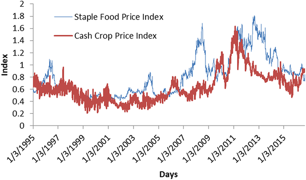
Figure 1. Daily movements of staple foods and cash crop price indices (2010 = 1).
4. Descriptive statistics and results
4.1. Descriptive statistics
The descriptive statistics of the price index return series are reported in Table 1. The statistics show that the food price index has the largest daily return and the lowest standard deviation, in comparison with the cash crop index. Overall, the series are asymmetric, with a small positive skewness, and have large kurtosis coefficients. The Jarque-Bera test statistics rejects the null hypothesis of normality for both price return indices. The ARCH test for heteroskedasticity points to the presence of the ARCH effect in both index series. Also, the Ljung-Box test for autocorrelation evidences the presence of autocorrelation. These results corroborate the use of an MGARCH model in assessing the volatility integration between cash crop and staple food markets. They are also in-line with the underlying characteristics of commodity price movements, notably volatility clustering, as described by Deaton and Laroque (Reference Deaton and Laroque1992). With respect to the stationarity of the series, ADF and the PP tests reject the null hypothesis of nonstationarity at the 1% level of significance. The unconditional correlation between cash and staple food price index using the Pearson coefficient is estimated to be 0.74 at the 5% level of significance.
Table 1. Descriptive statistics of the price index returns
Notes: Q(14) refers to the Ljung-Box test for autocorrelation of order 14. ARCH(14) is the Engle (Reference Engle1982) test for conditional heteroskedasticity of order 14, and the Jarque-Bera test is used to test for normality. The augmented Dickey-Fuller (ADF) and the Phillips-Perron (PP) methods are used to test for nonstationarity of the index series. ARCH, autoregressive conditional heteroskedasticity.
4.2. Results of the wavelet analysis
As discussed in Section 3, we use the Daubechies “extremal phase wavelets” to decompose the series into approximated and detailed series. The Daubechies family of wavelets is used in finance and economics because of their desirable properties of ortho-normality, asymmetry, and higher number of vanishing moments (Daubechies, Reference Daubechies1992). Figure 2 illustrates the decomposition exercise based on a multiresolution analysis (MRA) at various scales for both food and cash crop price indices. A maximum scale level j of 12 is selected, which is standard in the literature, because previous studies have shown that moderate filters are appropriate for financial data (Gençay, Selçuk, and Whitcher, Reference Gençay, Selçuk and Whitcher2001, Reference Gençay, Selçcuk and Whitcher2005; In and Kim, Reference In and Kim2013). Note that, according to Nyquist’s rule, half of the sample can be eliminated at each successive scale level. For illustrative purposes, we present three detailed series and one approximation series derived from the calculated values of the wavelet transform coefficients. A wavelet coefficient can be interpreted as the difference between two adjacent averages for a certain scale (Percival et al., Reference Percival, Wang and Overland2004). Practically, it shows how the average of a particular series changes when considering various scales (e.g., 2 days, 20 days, or 360 days). Analyzing the change in the average of price series at different scales helps detect any possible trends, discontinuities, or abrupt changes in the series. In Figure 2, the highest scale level (frequency) component d1 corresponds to a time-scale (frequency) of 21 = 2 days (daily effects), while d5 accounts for variations in a time-scale (frequency) of 25 = 32 days. The coarser, or smoother, part of the series (S7) captures the trend.
Figure 2. Wavelet decomposition results at selected scales for cash crop and staple food series. Note: “foodi” stands for food price index, and “cashi” represents the cash crop price index.
The MRA in Figure 2 suggests that the variations in the series are relatively heterogeneous across scales and time, with high fluctuations evidenced at finer-scale resolutions for both cash and staple food series. Some localized features are interesting to point out. For example, a stretch of high volatility toward the end of the sample is revealed for the staple food index, whereas there are marked variances at the start and toward the end of the sample for the cash crop price index, underpinned by large fluctuations in the value of the wavelet coefficients. The smooth series for the cash and staple food series (S7 in Figure 2) highlight the upward trend underlining both series up to their respective peak. Hence, the MRA suggests that the fluctuations in the decomposed series are heterogeneous across time and scales, implying that we can gain additional insights into the dynamics of the indices by considering their relationship at various scale levels. After obtaining the wavelet transform values, we proceed by denoising the series, as described in Section 3. Then, the series are reconstructed by adding to the trend, selected frequencies, or detail series, as described in equation (5). The selected scales (frequencies) are (1) low frequency (d = 9), (2) medium frequency (d = 5), and (3) high frequency (d = 1),Footnote 11 as illustrated in Figures 3 and 4.
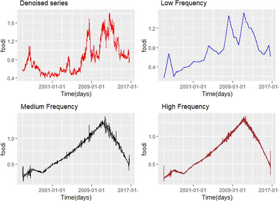
Figure 3. Reconstructed staple food price series at selected scales. Note: “foodi” stands for food price index.

Figure 4. Reconstructed cash crop price series at selected scales. Note: “cashi” represents the cash crop price index.
It is also possible to quantify how much each scale contributes to the overall variability of the index series through scale-based variance decomposition, as in Percival et al. (Reference Percival, Wang and Overland2004). The wavelet variance decomposition indicates that the largest contribution to the sample variance is accounted for by variations at the largest scale (long-run fluctuations) for both the cash crop and staple food indices. Hence, long-run variations have more weights on the series than short-run fluctuations.
In general, the results of the wavelet analysis show that the index series have common trends and volatility patterns, although differences in volatility prevail at specific scales. This suggests that the level of interdependence and the dynamics of volatility between cash crop and staple food price indices may vary depending on the considered timescale. As a result, we apply a BEKK-GARCH model using the denoised series at various time-frequency domains to account for the heterogeneity in the variance dynamics. This is described in the next section.
4.3. GARCH model
Using the staple food and the cash crop return indices, we estimate four bivariate VAR-BEKK-GARCH models. The first model uses the original series, whereas the other three models are applied to the denoised series but for different scale frequencies: low frequency (model 2), medium frequency (model 3), and high frequency (model 4). The VAR specification describes the conditional mean of the model, and the GARCH component explores the volatility interactions. We apply the AIC and SIC information criteria to identify the optimal lag order of the VAR system and run univariate GARCH for both index series to which we apply the same information criteria to examine the lag order for the GARCH component. The information criteria selects VAR(3) and GARCH(1,1) as the optimal specification. A comparative estimation of the log-likelihood values derived from other alternative lag specifications confirms the data are best characterized by a GARCH(1,1) specification.
The estimation results are reported in Table 2. The ARCH terms (a1i, a2i) indicate whether the conditional volatility is driven by lagged innovations, and the GARCH estimates (g1i, g2i) show if the current conditional volatility is influenced by its lagged values, reflecting volatility persistence. In general, estimation results for the four pairwise bivariate VAR(3)-BEKK-GARCH(1,1) models reveal some similar patterns with respect to the estimated ARCH and GARCH coefficients. First, the coefficients are found to be statistically significant for most of the pairwise estimations. Second, the estimated values for the ARCH coefficients are generally lower than the GARCH estimates, implying that lagged shocks do not affect current conditional variance as much as lagged volatility values. The diagnostic tests carried out on the standardized residuals and squared standardized residuals show a significant reduction in ARCH effects and autocorrelation depicted in the return series (see Table 1), indicating that the estimated models are sufficiently flexible to describe the volatility dynamics between staples and crop returns.
Table 2. Estimates of VAR(3)-BEKK-GARCH(1,1) for staple food and cash crop price indices at various time-frequency domains
Notes: A bivariate model VAR(3)–full-BEKK-GARCH(1,1) model is estimated for each model from January 2, 1990, to August 28, 2016. The information criteria AIC (Akaike information criterion) and SIC (Schwarz information criterion) were used to select the optimal lag order for the VAR model and the GARCH specification. Model 1: original series; model 2: low frequency; model 3: medium frequency; and model 4: high frequency. LB and LB2 are the Ljung-Box Q-statistic for standardized and standardized square residuals, respectively. P values reported in parentheses. Asterisk (*) stands for significant at the standard 5% level. Stationarity condition tests show that the estimated full BEKK-GARCH model is stationary. The estimates of matrix A (ARCH effects) and G (GARCH effects) shown in Table 2 are reported as expressed in equation (8). Note that we only show results for conditional variances. Estimated results for the conditional correlations are presented in Figure 5. ARCH, autoregressive conditional heteroskedasticity; BEKK, Baba, Engle, Kraft and Kroner; GARCH, generalized autoregressive conditional heteroskedasticity; VAR, vector autoregressive.
Table 2 also reports estimations for the mean price return equations. Results indicate that, generally, the own autoregressive parameters for both staple food and cash crop return indices are found to be statistically significant, implying short-term predictability. Results also show that some cross-market returns parameters are found to be positive and statistically significant, but their number is much less than in the case of own mean spillover estimates. Also, we note that the information transmission flows mostly from the staple food to the cash markets, as shown by the number of significant coefficients capturing the effect of changes in staple food crop returns on cash crop returns. This result may in fact reflect the relatively greater liquidity in the staple food futures markets relative to cash crop futures markets.
The diagonal elements of matrix A (see equation 7), which captures own shocks, and the diagonal elements of matrix G, associated with own GARCH effect, are significant for most of the estimated models. That is, own news and past volatility movements affect the current conditional variance values. Also, a general assessment shows that the off-diagonal elements of matrix A and matrix G are for most cases significant, but with some degree of variations, reflecting asymmetries in the dynamics. In terms of model 1 (i.e., original series), results are generally in-line with those obtained with the other models. For the staple food and cash crop equations, own ARCH and own GARCH terms are highly significant. In absolute terms, estimates of the ARCH coefficients are generally found to be much smaller than those obtained for the GARCH component, implying larger effects of past conditional variances than lagged innovations on current conditional variances.
For the low frequency model (i.e., long run), results indicate that the current conditional variance for cash crop return indices depends on their own ARCH and own GARCH terms, meaning that market volatility of cash crops can generally be predicted on the basis of past shocks and past variance. However, in contrast to model 1, the own ARCH effect is found to be larger than the own GARCH effect, suggesting that unexpected shocks play a much more important role in driving variability of staple returns at low frequencies. Likewise, the own ARCH estimate for staples and cash crop equations are found to be greater than the own GARCH effects for the medium-frequency model. In the case of the high-frequency model, the own GARCH effect is larger than the own ARCH effect for both the staple food and cash crop equations, in-line with the outcome obtained with model 1. That is, at high frequencies, the conditional variances of cash crop and staple food returns are influenced by their respective past variances more so than unexpected news.
We now turn our attention to volatility transmission between staple food and cash crops, which is captured by the cross-estimates of ARCH and GARCH terms. Overall, there is significant volatility transmission between staple foods and cash crops as evidenced by the number of significant cross-effects terms estimated for the various pairwise systems. We note that the cross-market GARCH estimates are generally much larger than those of the cross-market ARCH effects. This is an indication that the conditional volatility of cash crop (staple food) markets is largely influenced by periods of volatility in the staple food (cash crop) markets rather than by the effects of lagged price return innovations in the staple food (cash crop) markets. Specifically, the GARCH cross-market effects are all statistically significant, with the exception of model 1, where past volatility in the cash market is statistically insignificant in the staple food market, and the medium-frequency model, where the past volatility in the food market is statistically insignificant in the cash market. On the other hand, the cross-market ARCH effects are all statistically significant, with the exception of model 1, where past innovations in the staples market do not show a statistically significant influence on the volatility of cash crop returns. Overall, the results show that the absolute values of the estimated cross-market GARCH and ARCH estimates are generally higher and statistically significant in the low-frequency case than for the other frequency models, suggesting that the level of volatility interdependence between cash crop and staple returns is much stronger at lower frequencies. Further, the low-frequency model yields the largest Pearson correlation estimates, reflecting a tighter interdependence in the long run. The fact that the conditional correlations are larger at lower frequencies may suggest that external factors common to both markets, such as macroeconomic variables and world energy prices, explain the larger correlation in the long run. In the short run, commodity-specific factors (e.g., supply shocks affecting sugar crops) dominate movements in prices, a feature that underlines the lower conditional correlation between staples and cash crops. These results are also corroborated by the estimated conditional correlations, which indicate that the correlation at lower frequency is mostly positive and increasing in periods of high commodity prices (see Figure 5). Figure 5 also shows that as the frequency increases from low to high, the conditional correlation between staple and cash crop markets weakens. As mentioned, weaker volatility integration may be attributed to the influence of commodity-specific factors rather than common factors across staples and cash crops.
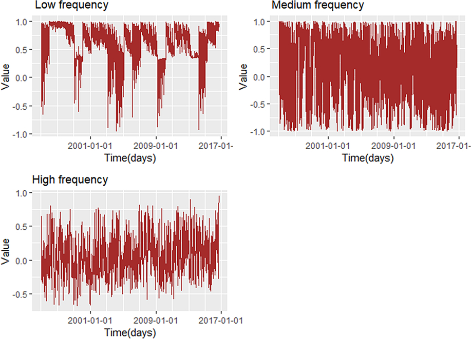
Figure 5. Estimated conditional correlation between the cash crop price index and the staple food price index at various time-frequency domains.
Estimation results also show that the cross-market values associated with the staple foods are generally larger than those relevant to cash crops. This means that information coming from the food markets influences cash crop markets to a larger extent than in the opposite direction, which could reflect the effect of greater liquidity underlying the staple food futures. The implication for LIFDCs is that market information relevant to staple foods affects ultimately the variability of cash crop earnings. Despite the bidirectional nature of the relationship, both the own GARCH and own ARCH effects are found mostly larger in magnitude than the cross effects, highlighting the dominant role of intrinsic market factors.
Figure 5 shows the estimated conditional correlations between staple food and cash crop return series at various timescales calculated following equation (10). The estimated values exhibit high volatility throughout the sample period, with values ranging between −0.5 and 0.5, notably for the medium- and high-frequency scales. In the case of the low-frequency model, conditional correlations fluctuate between 0.5 and 1, with occasional and abrupt changes mostly toward the negative values and periods of upward or downward trends.
Relatively high conditional correlation values associated with low-frequency scale implies that cash crop sales are a good hedge against increases in staple food import bills and can contribute to limiting current account instability in the long run, more so than in the short term. The extent to which export earnings offset current account deficits because of import bills depends on the elasticity of cash crop markets. The smaller the elasticity, the larger the increase in export earnings resulting from higher prices. What do these results mean for a country like Burundi, which relies on cash crop exports and imports of staple foods? Strong and positive conditional correlation between cash crop and staple food markets means that the government can evaluate more accurately its financial needs in the face of current account imbalances because of import bills by taking into consideration the fact that revenues from cash crop exports can reduce funding requirements and, hence, borrowing costs. Second, the government can also use price information relevant to international staple foods in the design and planning of investment strategies for the cash crop subsector, given the linkages between both commodity subsectors. For example, information on staple food price prospects can be utilized to strengthen the robustness of national cash crop price projections.
5. Conclusions and implications
The analysis carried out in this article examines the volatility interaction between staple food and cash crop futures price returns. The dynamics between these commodity groups is relevant for developing countries that depend on cash crop export earnings to address current account imbalances and sustain food imports. We apply a BEKK-GARCH framework supplemented by a wavelet analysis to locate precisely marked periods of volatility and changes in the dynamics at different time horizons.
Estimation results show that the GARCH and ARCH elements associated with the staple foods exhibit, for the most cases, larger absolute values than their corresponding elements related to cash crops. This implies that the information transmission takes place mostly from staple foods to the cash crop markets at the international level. When the GARCH framework is applied at different timescales, based on the wavelet transform analysis, the outcome reveals that the relationship between cash crop and staple foods is the strongest at the lower-frequency scale. The estimated conditional correlations for the lower-frequency model are mostly positive, with marked periods of upward and downward trends. Several studies attribute this synchronized behavior to the financialization of commodity markets, as investors seek to diversify market risks (Basak and Pavlova, Reference Basak and Pavlova2016; Grosche and Heckelei, Reference Grosche, Heckelei, Kalkuhl, von Braun and Torero2016). In the long run, however, comovement between staple food and cash crop markets can reflect changes in factor input costs, notably labor costs.
The results of our analysis convey some implications from both an investment and policy-making perspective. Because the correlation is found relatively higher in the long run, with significant cross-market effects, investors cannot use cash crop assets as a hedging strategy against holding staple food assets. However, the significance of the cross-market effects means that they can take into account information contained in staple food futures when predicting cash crop returns. From a policy perspective, the results imply that cash crop exports are a good hedge against rises in staple food import bills in the long run and can contribute to reducing current account instability. This is because higher cash crop prices imply higher export earnings, given the inelastic nature of international cash crop markets.
These results highlight the importance of the cash crop subsector as an automatic consumption smoother, in the face of increases in import bills. It is often argued, however, that developing countries should diversify away from commodity production and export. This reasoning is based on the observation that real commodity prices have been on a declining trend relative to the price of manufactures. The Prebisch-Singer hypothesis provides the theoretical background behind the decline in relative prices, which translates into deteriorating terms of trade for the developing countries (UNCTAD and FAO, 2017). Often, the recommended solution is to move away from the production and export of commodities, such as cash crops, and into more value-added products and services. The problem with this argument is that it is highly sensitive to the metrics used to derive real prices, in addition to the various issues related to trend estimation. Perhaps, the conclusion on whether to move away from commodity production and export should be looked at from several perspectives. As an example, the results of this article indicate that when comparing a cash crop price index relative to a staple food index, there is no obvious downward trend; in fact, the relationship between the indices seems to remain relatively steady in the long run, with prevailing short-lived peaks (see Figure A1 in the Appendix). Hence, when considering the movements of cash crop prices relative to staple foods, it appears that cash crop sales have a role to play in limiting the impact of higher staple food prices and the resulting current account instability. Perhaps better policy advice to cash-crop-producing developing countries would be to argue for more investment in the cash crop subsector so that it is more resilient and efficient, while at the same time, expanding the mix of exported products, particularly into more value-added products.
A number of conceptual and methodological aspects still require further investigation. First, although we apply a DWT to reconstruct the series into various timescales, the use of a CWT approach does not require the arbitrary selection of timescales and accounts endogenously for the presence of structural breaks. A CWT framework enables the measurement of the correlation between staples and cash crop returns in a continuous time-frequency domain. Future research could examine the interaction between cash crop and staples returns using CWT and compare the results with those obtained using a DWT method. Second, additional efforts are needed toward understanding the theoretical and empirical estimation of higher-dimension MGARCH models. Many of the statistical results still lack theoretical background to be generalized. Still, joint estimation of higher-dimension MGARCH models remains very interesting from a research aspect as it makes full use of the dynamics characterizing a system of variables. Finally, for these results to be translated at the country level, an assessment of the transmission of futures prices to export prices and import prices is warranted. This will help anticipate the extent to which a country’s cash crop export earnings can cover for food import bills given the volatile nature of international agricultural commodity markets.
Acknowledgements
The authors would like to thank the anonymous reviewers of this paper for constructive comments that helped improve the quality and content.
Financial support
This research was partially funded by European Union’s Horizon 2020 research project SUSFANS under grant agreement no. 633692.
Conflicts of interest
None.
Appendix
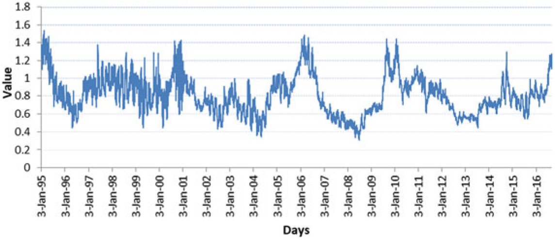
Figure A1. Cash crop price index versus staple food price index.
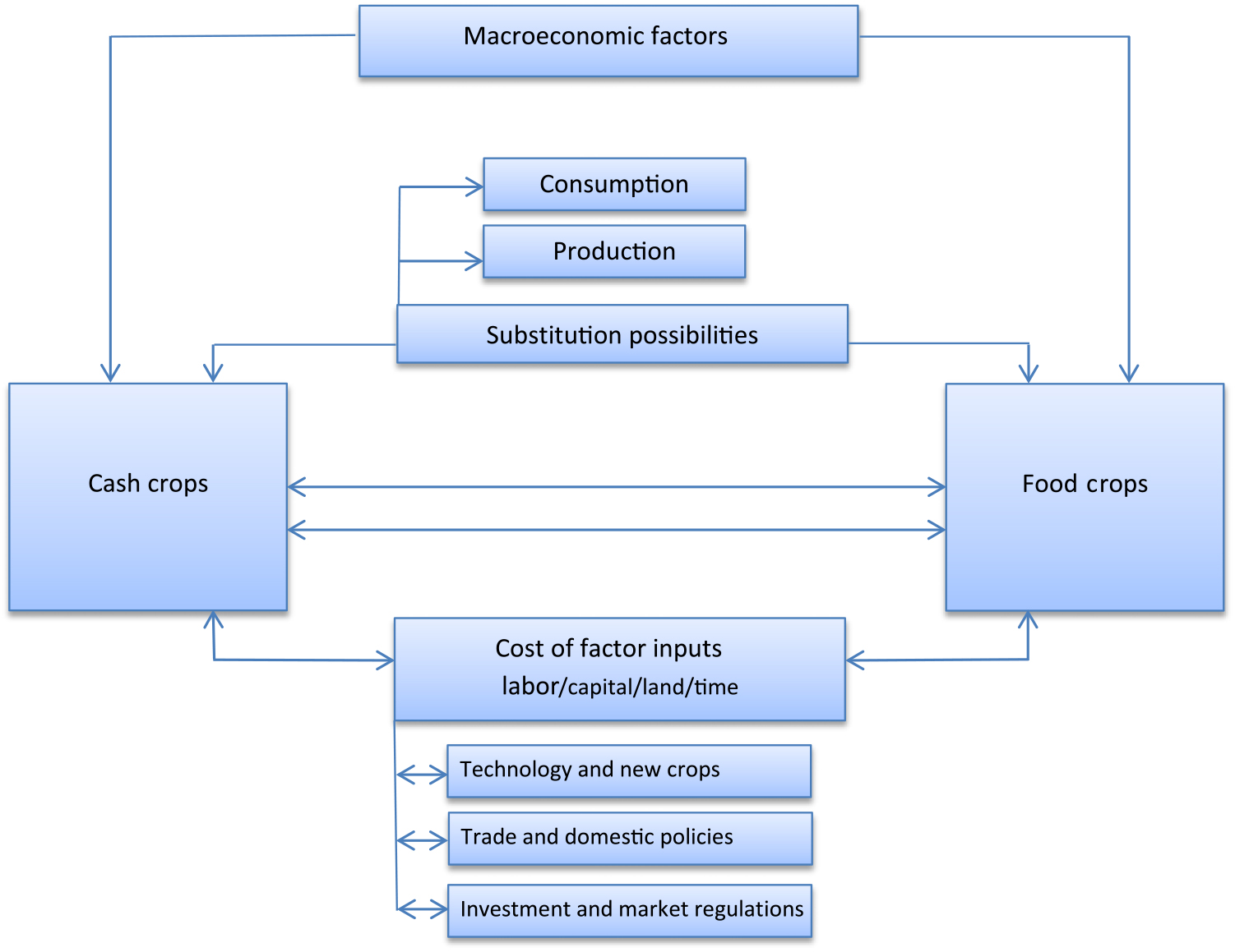
Figure A2. Interaction between cash crop and staple food prices: a conceptual framework. Notes: Aside from macroeconomic drivers, other underlying factors can cause cash crop and staple foods to correlate. These include factors related to the following: (1) changes in the cost of labor and other factors of production, (2) technological improvements and the introduction of a new farming activity that bids factor input costs, (3) trade and domestic policies, and (4) commodity investment and market regulations. Substitution possibilities in consumption and production between cash crops and staple foods in the physical market are rather limited and, hence, cannot explain the full extent of the price correlation.


 Open access