2 Annihilation processes and rates

Positrons in a magnetically confined pair plasma annihilate with: free electrons, bound electrons in the background gas and form short-lived bound states with electrons, positronium (Ps), which eventually annihilate. Collisions between positrons and other charged or neutral particles transport positrons towards the wall of the confinement chamber or, depending on the magnetic geometry, towards exposed magnets, e.g. in the case of a levitating dipole.

To compare the rates and spatial distribution of annihilation we need to choose a parameter range and magnetic confinement geometry. In this study the density–temperature space considered is in the range $0.01\,{\rm eV}\leq T \leq 5\,{\rm eV}$ and $10^{11}\,\mathrm {m}^{-3} \leq n \leq 10^{13}\,\mathrm {m}^{-3}$. This discussion uses the levitated dipole experiment as a reference for geometry and plasma parameters (figure 1). A levitating coil (orange in figure 1) produces a dipole field in a cylindrical chamber (black) with radius $a=20$ cm and height $h=26$ cm. While the equilibria of magnetized pair plasma have not yet been observed, electron–ion plasmas (Boxer et al. Reference Boxer, Bergmann, Ellsworth, Garnier, Kesner, Mauel and Woskov2010; Yoshida et al. Reference Yoshida, Saitoh, Yano, Mikami, Kasaoka, Sakamoto, Morikawa, Furukawa and Mahajan2013) as well as non-neutral electron plasmas (Saitoh et al. Reference Saitoh, Yoshida, Morikawa, Yano, Hayashi, Mizushima, Kawai, Kobayashi and Mikami2010) have been confined in levitating dipole fields and there have been theoretical calculations for thermal equilibrium of a non-neutral plasma in a dipole field trap (Steinbrunner et al. Reference Steinbrunner, O'Neil, Stoneking and Dubin2023) and maximum entropy states with adiabatic invariant constraints for a pair plasma in a dipole field (Sato Reference Sato2023). This discussion assumes a uniform density and temperature in a rectangular cross-section. While this profile ignores the observation of inward diffusion, resulting in a density profile peaked towards the magnet (Boxer et al. Reference Boxer, Bergmann, Ellsworth, Garnier, Kesner, Mauel and Woskov2010; Yoshida et al. Reference Yoshida, Saitoh, Morikawa, Yano, Watanabe and Ogawa2010), here, we are concerned with identifying gross annihilation profiles. The cross-section of the coil is square with $1.6$ cm sides centred at a radius of $7.5$ cm. The pair plasma is assumed to be confined within a rectangular cross-section (hatched blue) extending radially $5< r_p<19$ cm and axially $-6< z_p<6$ cm. The pairs on field lines intersecting the magnet are assumed to be lost, resulting in a plasma-free shadow around the magnet extending radially from $6.7 < r_s< 9.4$ cm and axially $-2 < z_s < 2$ cm.

Figure 1. Simplified geometry of a pair plasma in a levitating dipole. Floating coil (orange) of 7.5 cm radius levitates in a vacuum chamber (black outline). The pair plasma is assumed to be confined in a toroid with rectangular cross-section (blue hatched). The cross-section has a hole where field lines connect to the magnet. (a) Cross-section. (b) Top view.

Stoneking et al. (Reference Stoneking, Pedersen, Helander, Chen, Hergenhahn, Stenson, Fiksel, von der Linden, Saitoh and Surko2020) discussed positron annihilation with free and bound electrons as well as due to Ps formation in a magnetized pair plasma in terms of their effect on the lifetime of the pair plasma. Under ultra-high-vacuum conditions, when direct annihilation with bound electrons on neutrals and charge exchange become negligible, the main contributions to annihilation were found to come from Ps formation via radiative recombination and subsequent annihilation and direct annihilation with free electrons. At temperatures of several eV and higher, Ps formation through charge exchange with residual gas atoms may dominate the other processes but we will ignore this case here.

The mechanisms discussed so far originate in the bulk of the pair plasma. In a multi-species plasma there is transport towards boundaries such as the walls and magnet. Most positrons annihilate once they reach solid boundaries. Diffraction from low-energy positrons hitting solid surfaces is limited to no more than ${\sim }10\,\%$ of the incoming positrons (Rosenberg, Weiss & Canter Reference Rosenberg, Weiss and Canter1980; Schultz & Lynn Reference Schultz and Lynn1988) Here, we consider transport driven by Coulomb collisions and scattering off neutrals. In pair plasmas there is also the possibility of Ps-mediated transport where Ps forms, drifts across the magnetic field and ionizes either through collisions or fields, as has been studied for the case of antihydrogen in positron–antiproton traps (Jonsell et al. Reference Jonsell, van der Werf, Charlton and Robicheaux2009; Jonsell, Charlton & van der Werf Reference Jonsell, Charlton and van der Werf2016). Predicting transport processes in a plasma is difficult, but models can give estimates that can be checked by experiments. Scattering off neutrals is thought to be the main loss process in low-density positron confinement experiments (Horn-Stanja et al. Reference Horn-Stanja, Nißl, Hergenhahn, Pedersen, Saitoh, Stenson, Dickmann, Hugenschmidt, Singer and Stoneking2018). The measurements from these experiments can be scaled to the levitating dipole geometry. In a strongly magnetized plasma, where the Debye length $\lambda _D$ is longer than the Larmor radius $r_L$, collisions differ from classical plasma collisional theory. Due to the low densities, pair plasma will be strongly magnetized (Stenson et al. Reference Stenson, Horn-Stanja, Stoneking and Pedersen2017). Theory (Dubin & O'Neil Reference Dubin and O'Neil1997, Reference Dubin and O'Neil1998) and observations (Anderegg et al. Reference Anderegg, Huang, Driscoll, Hollmann, O'Neil and Dubin1997) in non-neutral plasma suggest the diffusion coefficient is enhanced for collisions with an impact parameter larger than the Larmor radius, $\rho > r_L$. For both transport processes, the diffusion rate is taken to be the annihilation rate.

Figure 2(a,b) shows the annihilation rates due to radiative recombination (green), direct (pink), Coulomb collision (yellow) and neutral collision (brown) processes in a magnetized pair plasma as a function of density and temperature (see the Appendix A for rate equations). The annihilation rate plotted is for all positrons in the volume $R=\varGamma N_{e^+}$, where $\varGamma$ is the annihilation rate of a single positron and $N_{e^+}$ is the initial number of confined positrons ($R$ is equivalent to the volume integral of source function over all space $\int f(\boldsymbol {x})\,{\rm d} V$). Here, $R$ represents an instantaneous rate of annihilation and gives a sense for how large the emission signal is from the plasma; this rate declines as the positron number depletes. However, since annihilation has been found to constrain the pair plasma lifetime to ${>}10^3$ s (Stoneking et al. Reference Stoneking, Pedersen, Helander, Chen, Hergenhahn, Stenson, Fiksel, von der Linden, Saitoh and Surko2020), $R$ approximates the rate during the first seconds or minutes of confinement and we will not consider the time dependence of the source distribution. Below the targeted pair plasma regime densities ($n<10^{11}\,{\rm m}^{-3}$), these plasma are transport limited; diffusion to material surfaces due to neutral collisions dominates the other annihilation processes by several orders of magnitude. Transport due to Coulomb collisions as well as the rates of radiative recombination and direct annihilation increase with density faster than transport due to neutral collisions. While the ratio between direct annihilation and radiative recombination is independent of density, the positron density does affect their respective ratios to transport processes. Diffusion due to Coulomb collisions will overtake diffusion due to neutral collisions around $n \sim 10^{12}\,{\rm m}^{-3}$ and radiative recombination around $n \sim 9 \times 10^{12}\,{\rm m}^{-3}$. This suggests that positron annihilation lifetime spectroscopy measurements (Cassidy et al. Reference Cassidy, Deng, Tanaka and Mills2006) of a $n=10^{13}\,{\rm m}^{-3}$ pair plasma may see two distinct loss regimes as the plasma decays.

Figure 2. Annihilation rates $R$ due to direct pair collisions (pink), radiative recombination (green), Coulomb collision diffusion (yellow) and neutral collision diffusion (brown) in a 12 litre pair plasma in the simplified dipole confinement geometry. (a) Density dependence of annihilation rates $R$ of a pair plasma with temperature $1$ eV. The grey region marks the targeted densities for low-energy pair plasma experiments. (b) Temperature dependence of annihilation rates of a pair plasma with density $10^{12}\,{\rm m}^{-3}$. (c) Ratio of neutral collision diffusion to Coulomb collision diffusion over density–temperature space. (d) Ratio of the rate of radiative recombination to the rate of Coulomb collision diffusion over density–temperature space.

Annihilation of free positrons with electrons results in the production of two gammas most of the time. The resulting 2$\gamma$ signal from direct annihilation is volumetric, extending across the plasma volume (figure 3a,b).

Figure 3. Spatial distribution of annihilation events in one second in $1$ eV, $12$ litre pair plasma with density $10^{12}\,{\rm m}^{-3}$ magnetically confined in the dipole field of a levitating dipole as shown in figure 1: (a,b) direct annihilation events between positrons and free electrons resulting in 2$\gamma$ emission, (c,d) 2$\gamma$ decays of positronium, (e,f) 3$\gamma$ decays of positronium, (g,h) 2$\gamma$ emission from annihilation of positrons diffusing from the plasma to magnet and limiter.

At the assumed temperatures and densities, the most significant Ps formation channel is radiative recombination. The lifetime and decay of Ps depends on the spin of the bound particles (Ore & Powell Reference Ore and Powell1949; Deutsch Reference Deutsch1951). Parapositronium (pPs) has antiparallel spins and its ground state decays into two gammas with an mean lifetime of $125$ ps. Orthopositronium (oPs) has parallel spins and its ground state decays into three gammas with a mean lifetime of $142$ ns (Vallery, Zitzewitz & Gidley Reference Vallery, Zitzewitz and Gidley2003). With a $1$ eV temperature the ground state of pPs (oPs) can travel $5\,\mathrm {\mu }$m ($6$ cm) in its mean lifetime at the most probable speed ($\sqrt {kT/m_e}$). There is also a small probability of creating $2n$ or $2n+1$ photons, although the branching ratio for the 4 and 5 gamma decays is of the order of $10^{-6}$ and declines further for higher $n$ (Karshenboim Reference Karshenboim2004). For unpolarized positrons $1/4$ of the Ps formation will be pPs and $3/4$ oPs. Ps may form in excited states with probabilities and lifetimes discussed in the Appendix and Appendix tables 1 and 2 (Gould Reference Gould1972, Reference Gould1989; Alonso et al. Reference Alonso, Cooper, Deller, Hogan and Cassidy2016; Cassidy Reference Cassidy2018). Magnetic fields can lead to Zemann mixing of singlet and triplet states, which will reduce oPs lifetimes, however, we do not consider this effect (Deutsch & Dulit Reference Deutsch and Dulit1951; Alonso et al. Reference Alonso, Cooper, Deller, Hogan and Cassidy2015). Ps propagates freely at the chosen velocity until either the end of its lifetime or it intersects a solid object, i.e. the wall or magnet. The annihilation signal and location are determined by which state of Ps forms and where the Ps ’walks to’. To model the spatial distribution of annihilation due to Ps formation, we

1. (i) randomly distribute formation events over the uniform plasma volume;

2. (ii) determine the energy state and the corresponding lifetime (or for higher energy state the total lifetime of the state cascade) using the lifetimes in tables 1 and 2;

3. (iii) pick each of the three velocity components from a normal distribution centred at $0$ with $\sigma =\sqrt {kT/(2m_e)}$;

4. (iv) propagate the Ps along its velocity direction using a $1$ mm step size according to its lifetime and speed;

5. (v) check for intersections with solid objects.

Table 1. Population of S states and their respective lifetimes after pPs formation in states up to $n = 4$.

Table 2. Population of S states and their respective lifetimes after oPs formation with states up to $n = 4$.

The resulting 3$\gamma$ signal from oPs is volumetric, extending throughout the chamber (figure 3e,f). There is a gradient in the 3$\gamma$ source density outside the plasma volume. The oPs intersecting the wall or magnet can interact with solids in multiple ways, including pick-off and quenching to para-positronium, that lead to fast decay and enhanced 2$\gamma$ decay probabilities (Schoepf et al. Reference Schoepf, Berko, Canter and Sferlazzo1992; Coleman Reference Coleman2002; Cassidy Reference Cassidy2018). We assume all wall and magnet intersections to contribute to the 2$\gamma$ signal along with pPs decays (figure 3c,d). The 2$\gamma$ signal from Ps is confined essentially to the plasma volume with the exception of longer lived excited pPs states that can drift out and the oPs that reaches the wall and magnet. The positron transport results in a localized annihilation signal from the magnet and from a narrow, ${\sim }2$ cm in axial extent, azimuthal ring where the field lines intersect the wall. We assume the transport has no inward/outward preference so that half of the annihilation occurs on the magnet and half on the wall. The signal can be made more localized if a circular limiter ($1.3$ cm radius, $5$ mm in front of wall at $y=0$ and positive $x$) is introduced (figure 3g,h).

Examining the photon counts further constrains the source distribution $f(\boldsymbol {x})$. Photon counts can be differentiated between the count of all photons, $\gamma$, and the count of photon pairs from 2$\gamma$ emission, $\gamma _2$. The latter can be diagnostically identified by their distinct energy signature (511 keV). Another classification is in terms of the photon origin, denoted by subscripts: $\gamma _{{\rm vol}}$ for photons emitted from volumetric sources, $\gamma _{{\rm bds}}$ for photons emitted from Ps hitting boundaries and $\gamma _{{\rm diff}}$ for photons emitted when diffusing positrons hit the narrow field-line intersections of the magnet and wall or limiter. The latter two origins only contribute to the $\gamma _2$ count since, in our model, annihilation on solids results in 2$\gamma$ events. The majority of the photons emitted originate from diffusion for much of the parameter space, making the quantification of diffusion processes a promising diagnostic aim (figure 4a). In dense and cold pair plasmas $\gamma _{2{\rm vol}}$ can exceed 20 % of the total $\gamma _2$ but for a large portion of the density–temperature space, the fraction is less than 1 % (figure 4b). The 2$\gamma$ emission can be detected by coincidence, which is highly localized to the magnet and limiter. A suitable arrangement of detectors can create LOR that do not cross the diffusion emission regions. These LOR will only cross a small fraction of the wall and a large fraction of the volume. The ratio of volumetric 2$\gamma$ photons to 2$\gamma$ photons emitted at the boundaries excluding the diffusion photons, $\gamma _{2{\rm vol}}/(\gamma _2 - \gamma _{2{\rm diff}})$, stays above 40 % throughout the density–temperature space (figure 4c). The volumetric and localized signals indicate that, even with multiple overlapping processes, we can likely untangle their contributions. There are four signals that are of particular interest:

1. (i) Transport provides emission that is strongly localized to the magnet and wall section or limiter and that has the dominant photon count for much of the parameter space. The magnitude of this signal is directly related to the physics of transport/diffusion processes. The strong localization lends itself to a diagnostic method exploiting distance attenuation.

2. (ii) The volumetric 2$\gamma$ emission that can be filtered due to its distinct energy. This emission is due to direct annihilation and Ps formation (pPs) which are both related to the density and temperature profiles of the pair plasma. The volumetric 2$\gamma$ signal is dominated by the transport emission which is 2$\gamma$ as well. A suitable choice of detector positions could have LORs with good sampling of both, allowing for tomographic reconstruction of the volumetric 2$\gamma$ emission source.

3. (iii) The 2$\gamma$ signal is localized and related to the positronium (oPs) formation and thermal drift. Diagnosing this signal with LORs with a long path along the wall may help disentangle the contribution of Ps formation and direct annihilation in signal 2.

4. (iv) The volumetric 3$\gamma$ emission from the oPs decay. The magnitude of this signal is directly related to the positronium formation rates. This signal can be diagnosed by examining its effect on the gamma energy spectrum (Alkhorayef et al. Reference Alkhorayef, Alzimami, Alfuraih, Alnafea and Spyrou2011) and from triple coincidence detections (Moskal et al. Reference Moskal, Gajos, Mohammed, Chhokar, Chug, Curceanu, Czerwiński, Dadgar, Dulski and Gorgol2021).

Figure 4. Emission fractions. (a) Ratio of total number of photons emitted due to diffusion ($\gamma _{{\rm diff}}$) to all photons emitted ($\gamma$). These ratios account for 2$\gamma$ and 3$\gamma$ emission. (b) Ratio of volumetric 2$\gamma$ ($\gamma _{2{\rm vol}}$) photons to total 2$\gamma$ photons emitted ($\gamma _2$). (c) Ratio of volumetric 2$\gamma$ ($\gamma _{2{\rm vol}}$) photons to total 2$\gamma$ photons emitted minus the diffusion photons ($\gamma _2 - \gamma _{2{\rm diff}}$).

3 Gamma-detector array sensitivity

Here, we introduce the gamma-detector array, evaluate its sensitivity function $a(\boldsymbol {x})$ of (1.1), quantify its time and energy resolution and discuss the effect of these quantities on measurement capabilities. Radioisotope sources are used as effective point sources of emissions to characterize detection systems. For single photon counting from a point source of emission ($f(\boldsymbol {x}) \rightarrow R\delta (x)$) we approximate the integral over the FOV as the multiplication of the solid angle of the source covered by the detector(s) $\varOmega$ with the efficiency factor $\eta$, which includes the detector efficiency as well as all other physics such as attenuation and scattering over all space

(3.1)\begin{equation} C_i = \int_{{\rm FOV}} a_i(\boldsymbol{x}) R \delta(\boldsymbol{x}) \,{\rm d}\boldsymbol{x} \sim \varOmega_i(\boldsymbol{x}) \eta_i(\boldsymbol{x}) R. \end{equation}

In practice, $\eta$ is determined for both the total counts of a detector and the counts in the photo-peak (with subscript $pp$) as the provenance of the latter as non-scattered emission is more certain. We now proceed to evaluate the solid angle coverage $\varOmega _i$ based on the detector geometry and use reference ${}^{22}\mathrm {Na}$, $\beta +$ emitters, to determine $\eta$; ${}^{22}\mathrm {Na}$ emits prompt $1274.5$ keV gammas and positrons. The source is wedged between two $3\,\mathrm {mm}$-thick Teflon sheets to ensure that most positrons will annihilate close to the source into two gamma rays. A 3D-printed sample holder aligns the source to the vertical centres of the detectors.

We use a test set-up (figure 5) with 16 BGO (Scionix 25B25/1M-HV-E2-BGO-X2) detectors arranged in a circle with radius $r_d=33$ cm, which could also fit the 48 detectors ($16.7\times 3.97$ cm) envisaged for the pair plasma experiments. Each detector consists of a cylindrical BGO crystal with $2.54$ cm diameter and $2.54$ cm length. The solid angle coverage of a circular detector to a point source along the axis of detector is given by (Knoll Reference Knoll2010)

(3.2)\begin{equation} \varOmega = 2{\rm \pi} \left( 1 - \frac{\ell}{\sqrt{\ell^2 + \alpha^2}} \right), \end{equation}

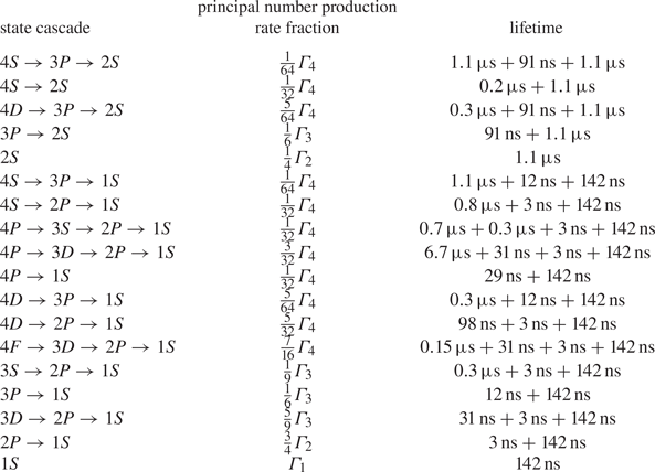
where $\ell =\lvert \boldsymbol {r}_i - \boldsymbol {x} \rvert$ is the distance between the detector and the source and $\alpha$ is the radius of the scintillator. We use (3.2) to estimate the solid angle coverage for sources inside a $20$ cm radius corresponding to the assumed plasma extent. Figure 6(a) shows the solid angle coverage of the detector arrangement, summing the solid angle coverage of all 16 detectors for point source positions on a $1$ mm grid. The $4{\rm \pi}$ coverage varies from $0.6\,\%$ to roughly $1\,\%$ at the edges. Figure 6(b) shows the solid angle coverage of the pairs of detectors forming lines of response. For coincident detection the solid angle for each source point is determined by the detector furthest from the source. The maximum solid angle coverage for coincidences is the centre where the most (8) lines of response meet. There are several locations with no lines of response and consequently no solid angle coverage.

Figure 5. Test set-up imitating annihilation in a toroidal magnetic confinement geometry. Sixteen BGO detectors are equally spaced (every $22.5^\circ$) at $33$ cm radius ($r_d$) around a ${}^{22}\mathrm {Na}$ source (white square at $r_s$) placed on turntable with a 22.5 cm radius ($r_t$).

Figure 6. The $4 {\rm \pi}$ coverage of the 16 detectors (blue squares) arranged in a $33$ cm radius circle. (a) Sum of solid angle coverage of all detectors for single photons emitted by point source located inside a radius $20$ cm. (b) Sum of solid angle coverage for two photon coincidence emitted by a point source located inside a radius $20$ cm.

The triple coincidence photons from oPs decay and from the $2\gamma$ annihilation and $1274.5$ keV photon of the ${}^{22}\mathrm {Na}$ decay have different angular correlations. While momentum conservation ensures that the 3$\gamma$ from oPs decay are nearly co-planar (Moskal et al. Reference Moskal, Gajos, Mohammed, Chhokar, Chug, Curceanu, Czerwiński, Dadgar, Dulski and Gorgol2021), the angle of the $1274.5$ keV is arbitrary with respect to the $2\gamma$ LOR. Here, we only briefly discuss the former as it is relevant to pair plasma diagnostics. We can estimate the solid angle coverage for a triple coincidence by calculating the solid angle for the detection of two arbitrarily directed $\gamma$ and a third $\gamma$ propagating in the plane defined by the first two $\gamma$, so within the cylinder ($r_d=33$ cm) partially covered by the 16 detectors with radius $\alpha$. The $4{\rm \pi}$ coverage at the centre is $\varOmega _{3\gamma }(r=0)/(4{\rm \pi} ) \sim (0.6\,\%)(0.6\,\%)(16 \alpha ^2 {\rm \pi})/(2 {\rm \pi}r_d 2\alpha ) \sim 0.0006\,\%$.

The detection efficiency as well as nonlinear aspects of the response i.e. the rate of false coincidences and missed counts, are influenced by the hardware. Scintillation in the detectors is converted to electrical pulses with photo-multipliers (Hamamatsu 1924A) and preamplifiers with heights proportional to the absorbed photon energy. The output pulse from the preamplifiers has a rise time of $140$ ns and a decay time of $1\,\mathrm {\mu }$s. Field-programmable gate array (FPGA) based multi-channel analysers (CAEN V1730S) digitize all detector outputs to 14 bit resolution at 500 MS s$^{-1}$. The FPGA timestamps the $50\,\%$ of peak amplitude point of each pulse with a digital implementation of a constant-fraction (CFD) trigger and determines the pulse height by digitally integrating a set gate of $150$ ns before and $1850$ ns after the trigger. During the decay of the pre-amplifier the signal remains above the threshold of the CFD trigger, resulting in a dead time $t_D \sim 4\,\mathrm {\mu }$s. The fraction of the measured rate to the true rate $R_m/R_t$ can be estimated (Knoll Reference Knoll2010) as $R_m/R_t = 1 - R_m t_D$. Missed events due to dead time will be significant and need to be accounted for, as the missed counts start to exceed 1 % of the measured rate when $R_m > 2.5 \times 10^3$ Hz. This dead time does not affect coincidence measurements as these occur on two separate detectors.

We measure the time resolution in order to estimate the rate of false coincidences. Figure 7(a) shows the time intervals between consecutive detection events by the 16 detectors when a ${}^{22}\mathrm {Na}$ source is placed in the centre. The count rate and time are normalized by the activity of the source. The distribution of intervals between events for all detectors fits an Erlang distribution, except for the leftmost bin, which is over-populated due to coincident detections between pairs of detectors for 2$\gamma$ annihilations. Binning for these shortest time intervals reveals that the coincident intervals fit a Gaussian distribution with standard deviation of $8$ ns, which is the time response of the detection system. We treat detections within three standard deviations as coincident, giving a coincidence window $\tau =24$ ns. The FPGA has been shown to be able to timestamp the square pulses from a delay generator (SRS DG645) to the accuracy of the generator ($1$ ns) so the time response is dominated by the electronics of the BGO detector package. The fraction of false coincidences can be estimated (Parker et al. Reference Parker, Forster, Fowles and Takhar2002) as $R_{fc}/R_m \sim 2 \tau R_m$. $R_{fc}/R_m \sim 1\,\%$ with $R_m=2\times 10^5$ Hz; given the solid angle coverage (figure 2a), the predicted rates of annihilation should result in few false coincidences.

Figure 7. Frequency of intervals between successive detections on (a) total rate and (b) coincidence time scale. The count rates and intervals (in (a) but not (b) are normalized by the source activity $\bar {C}=C/R$ and $\bar {{\rm \Delta} t}={\rm \Delta} t \cdot R$, where $R=35$ kBq. On long time scales the interval distribution fits an Erlang distribution (dashed orange). On nanosecond time scales the distribution of intervals fits a Gaussian distribution (dashed orange) with a standard deviation of $\sigma =8\,\mathrm {ns}$.

Characterizing the energy resolution of the detector array allows us to estimate how well we can filter for $511$ keV photons and how well we can relate counts to the annihilation rate. Figure 8(a) shows the energy spectrum of single detections calibrated with the ${}^{22}\mathrm {Na}$ peaks at $511$ and $1274.5$ keV. The $511$ keV photo-peak can be fitted by a Gaussian distribution on top of a continuum fitted with an exponential decay (dashed orange) (Knoll Reference Knoll2010). Comparing the ratio of the signal in the continuum and the 511 keV peak produced by the annihilation of the pair plasma can provide an estimate of the oPs formation rate, as the 3$\gamma$ annihilation will increase the number of detections in the lower-energy ‘valley’ (Alkhorayef et al. Reference Alkhorayef, Alzimami, Alfuraih, Alnafea and Spyrou2011). The FWHM of the $511$ keV annihilation peak is 13 % for gamma spectra acquired in this study, corresponding to a 66 keV energy resolution (Karwowski et al. Reference Karwowski, Komisarcik, Foster, Pitts and Utts1986). Figure 8(b) shows the energy spectrum of coincident detections within 24 ns on two detectors $i$ and $j$. ${}^{22}\mathrm {Na}$ emits 1274.5 keV photon within picoseconds of the positron emission so there can be coincidences between the $511$ keV photons from 2$\gamma$ annihilation, as well as the $1274.5$ keV photons and the partial absorption of photons due to Compton scattering.

Figure 8. Energy spectrum from 16 BGO detectors forming a 33 cm radius circle around a ${}^{22}\mathrm {Na}$ source. The count rate is normalized by the source activity $\bar {C}=C/R$, where $R=35$ kBq. (a) Energy spectrum of single photon detections. The spectrum around the $511$ keV photo-peak can be fit by a Gaussian and an exponential (dashed orange). (b) Energy spectrum of coincident detections on two detectors $i,j$ within $\tau =24$ ns.

We measure $\eta (\boldsymbol {x})$ by comparing the experimental counts from three ${}^{22}\mathrm {Na}$ sources with (3.1) and taking into account that $f$ is the known source activity adjusted for the photons emitted per decay, which is $0.999+1.798$ for all counts and $1.798$ for 511 keV photon peak counts (Delacroix et al. Reference Delacroix, Guerre, Leblanc and Hickman2002); $\eta ({\boldsymbol {x}})$ depends logarithmically on the distance between the source and the detector. For positions on the turntable, $\eta$ varies between 6 and 7 and $\eta _{pp}$ varies between 0.4 and 0.45. In a pair plasma experiment the stainless steel chamber walls and other components will attenuate radiation, necessitating care in calibrating the detection system for a spatially varying factor $\eta (\boldsymbol {x})$.

4 Diagnostic methods

4.1 Distance-attenuated photon counting of transport

Figure 3(g,h) shows that diffusion in a pair plasma could result in a ring of annihilation on the magnet and localized annihilation on a limiter. A distance-attenuation calibration of the gamma-detector array can identify the diffusion emission on the limiter. By placing a ${}^{22}\mathrm {Na}$ source at 8 different radii, a count function can be fitted to the measurements at each detector

(4.1)\begin{equation} \bar{C}_i = A \left( 1 - \frac{\ell}{\sqrt{\ell_i^2 + \alpha^2}} \right) + \beta, \end{equation}

where the fitted parameters are $A=7.27 \pm 0.04$ and $\beta =(6.7 \pm 0.2) \times 10^{-4}$ (figure 9). The fit shows that at positions within the $20$ cm ‘plasma’ radius discrepancies with the model (3.2) assumptions, due to the point source being off axis from the detector planes, are small.

Figure 9. Identification of localized $\gamma$ source off axis of an axisymmetric distribution of $\gamma$ emission as an approach for identifying pair plasma diffusion onto a limiter. (a) Calibration of distance-attenuated photon count rate. Blue dots are counts per second recorded on detectors a distance $\ell$ from the source. The measurements fit (4.1) (dashed orange). (b) The counts rate on each of the 16 detectors recorded with a $\gamma$ emission distribution $f(x)=\delta (r-r_0)$, with $r_0=7$ cm. (c) The counts rate on 16 detectors with a $\gamma$ emission distribution $f(x)=E \delta (x)\delta (y-y_o) + F \delta (r-r_0)$, where $y_0=-20$ cm and $E$ and $F$ are rate constants. The expected counts for a point source at $y=-20$ cm is shown in dashed red. The count rate is normalized by the source activity $\bar {C}=C/R$, where $R=35$ kBq.

A pair plasma diffusion-like source distribution can be approximated with $f(x)= E \delta (x)\delta (y-y_0) + F \delta (r-r_0)$, where $y_0=-20$ cm, $r_0=7$ cm and $E$ and $F$ are constants characterizing the rate of the point and circular emission. This $f(x)$ can be simulated with ${}^{22}\mathrm {Na}$ source $7$ cm off centre on the turntable to simulate the circular emission profile and a stationary ${}^{22}\mathrm {Na}$ source at $y=-20$ cm to simulate the emission from a limiter. An equal transport fraction can be simulated by acquiring counts from the same source and for equal time at each source position. The emission from an axisymmetric source coaxial with the gamma detector results in an approximately equal count on all detectors with differences up to 13 % due to variance in the detector efficiency (figure 9b). Measurements of a known source located at the centre can be used to calibrate these count differences. The emission from the ‘limiter’ source at $y_0=-20$ cm can be identified by determining the count fraction expected on each detector (red dashed in figure 9(c). The residual difference between the expected counts and the actual counts above the adjusted axisymmetric counts is 3 %. This demonstrates that the fractional single photon counts on a detector array can identify the counts from a localized source in the presence of an axisymmetric background. The localized emission rate can be estimated from a least-squares fit to the detector photon counts.

4.2 Tomographic reconstruction of volumetric coincidence sources

Equation (1.1) gives a set of linear equations that can be solved for the emission source distribution. For coincident counts $C_{ij}$ of detectors $i$ and $j$ we can express the equation set as a matrix multiplication with $N=16\times 16 = 256$ rows, one for each detector pair. Denoting matrices in bold,

(4.2)\begin{equation} \textit{C} = {\mathsf{A}} \boldsymbol{\cdot} \textit{f}. \end{equation}

${\mathsf{A}}$, the system response function incorporates effects such as the sensitivity of the detectors, non-collinearity due to pair momentum, scattering and attenuation (Baker, Budinger & Huesman Reference Baker, Budinger, Huesman, Pilkington, Loftis, Palmer and Budinger1992). Here, ${\mathsf{A}}$ has dimensions $M \times N$, where $M$ is the number of discretized locations inside the $20$ cm confinement space. We choose $M=96 \times 96 = 9216$. There are several strategies for inverting these equations and choices for basis functions for the reconstructed distribution, e.g. sinusoids in the filtered back projection algorithm (Hobbie & Roth Reference Hobbie and Roth2015).

Figure 10(a–c) shows the counts on the LOR matrix for distribution functions simulating the diffusion onto the magnet ($f \propto \delta (r-r_0)$ with $7\,\mathrm {cm}$), the pair plasma ($f \propto \delta (r-r_0)$ with $r_0=15\,\mathrm {cm}$) and the limiter ($f \propto \delta (x)\delta (y-y_0)$ with $y_0=-20\,\mathrm {cm}$). There are no coincident counts on the same detector $i=j$, since the dead time is longer than the coincidence interval (24 ns). Axisymmetric distributions appear as off-diagonal lines in the count matrices. The limited number of diagonals with 16 detectors indicates that the radial resolution is limited. To invert the coincident counts, we estimate the system response matrix by tallying the intersections of uniformly discretized in-plane emission angles ($10^5$ angles) with the detectors. This is done for point sources at each of $96 \times 96$ discretized locations. The resulting matrix is sparse (${>}95$% of entries are zero) and can be pseudo-inverted (Penrose Reference Penrose1955) with a singular value decomposition (SVD) ${\mathsf{A}}={\mathsf{U}} {\mathsf{S}}{\mathsf{V}}^{\ast } \Rightarrow {\mathsf{A}}^+={\mathsf{V}} {\mathsf{S}}^{-1} {\mathsf{U}}^{\ast }$, where ${\mathsf{U}}$ is a unitary matrix with $M\times M$, ${\mathsf{S}}$ a diagonal matrix and ${\mathsf{V}}$ the conjugate transpose of a unitary matrix with $N \times N$ elements. The $K=100$ largest values are used for this pseudo-inversion. The source distribution can then be reconstructed with the dot product of the pseudo-inverse ${\mathsf{A}}^+$ and the detector counts $\textit{{C}}$,

(4.3)\begin{equation} \textit{f} = \textit{C} \boldsymbol{\cdot} {\mathsf{A}}^+. \end{equation}

Figure 10(d–f) shows the reconstructions based on the count matrices. Reasonable reconstructions require approximately $10^6$ coincident counts, which is reasonable for a large part of the density–temperature space (figure 4a) and the solid angle coverage (figure 6b). Artefacts (resembling the coincident solid angle coverage figure 6b) are visible due to the coarse sampling of the area with LORs between only 16 detectors. Toroidally averaging the two-dimensional reconstructions gives radial profiles, removing the artefacts and requiring fewer counts, ${\sim }10^4$ (figure 11). The resolution is limited by the number of detectors to a few cm as indicated by the width of the peaks in the radial profiles. The results shown here demonstrate that the coincident counts from a gamma-detector array can be used to reconstruct an emission profile similar to that expected from a magnetically confined pair plasma. Volumetric emission can be differentiated from the dominant emission due to diffusion with appropriate placement of LORs.

Figure 10. Coincident counts and 2$\gamma$ emission profile reconstructions of source distribution functions noted in titles. (a–c) Relative fraction of coincident counts on each detector pair $i, j$. (d–f) Reconstruction of emission profile calculated by multiplying coincident count vector with inverse of system response matrix A.

Figure 11. Radial profiles from tomographic reconstruction of the source distribution function noted in legend. The blue and orange lines are toroidal averages and the green line is a toroidal sum of the two-dimensional reconstruction of the respective source distribution.